The Milky Way has no thick disk

Abstract

Different stellar sub-populations of the Milky Way’s stellar disk are known to have different vertical scale heights, their thickness increasing with age. Using SEGUE spectroscopic survey data, we have recently shown that mono-abundance sub-populations, defined in the $[\alpha\mathrm{/Fe}]$-$[\mathrm{Fe/H}]$ space, are well described by single exponential spatial-density profiles in both the radial and the vertical direction; therefore any star of a given abundance is clearly associated with a sub-population of scale height $h_{z}$. Here, we work out how to determine the stellar surface-mass density contributions at the solar radius $R_{0}$ of each such sub-population, accounting for the survey selection function, and for the fraction of the stellar population mass that is reflected in the spectroscopic target stars given populations of different abundances and their presumed age distributions. Taken together, this enables us to derive $\Sigma_{R_{0}}(h_{z})$, the surface-mass contributions of stellar populations with scale height $h_{z}$. Surprisingly, we find no hint of a thin-thick disk bi-modality in this mass-weighted scale-height distribution, but a smoothly decreasing function, approximately $\Sigma_{R_{0}}(h_{z})\propto\exp(-h_{z})$, from $h_{z}\approx 200$ pc to $h_{z}\approx 1$ kpc. As $h_{z}$ is ultimately the structurally defining property of a thin or thick disk, this shows clearly that the Milky Way has a continuous and monotonic distribution of disk thicknesses: there is no ‘thick disk’ sensibly characterized as a distinct component. We discuss how our result is consistent with evidence for seeming bi-modality in purely geometric disk decompositions, or chemical abundances analyses. We constrain the total visible stellar surface-mass density at the Solar radius to be $\Sigma^{{}^{*}}_{R_{0}}=30\pm 1\ M_{\odot}$ pc^-2.

1. Introduction

In both the Milky Way (Gilmore & Reid, 1983) and external galaxies (Tsikoudi, 1979; Burstein, 1979), the stellar-density or luminosity profiles perpendicular to the disk plane reveal an excess over a simple exponential “thin disk” at distances $|z|\gtrsim$ 1 kpc. This excess, confirmed by many studies in the last two decades (e.g., Reid & Majewski, 1993; Jurić et al., 2008), seems to be a generic feature of galactic disks (e.g., Yoachim & Dalcanton, 2006) and has typically been described by, and often ascribed to, the presence of a “thick-disk” component, distinct from both the halo and thin disk components (e.g., Jurić et al., 2008). However, whether or not the excess is sensibly attributed to a distinct “thick-disk” component is, in our view, an open question (see $\mathsection$ 1.1).

Studies of the age, kinematics, and elemental-abundance ratios of probable members of the thicker disk component have revealed that it is older (e.g., Bensby et al., 2005), kinematically hotter (e.g., Chiba & Beers, 2000), and metal-poor and enhanced in $\alpha$ elements (e.g., Fuhrmann, 1998; Prochaska et al., 2000; Lee et al., 2011). Recent analyses (Navarro et al., 2011; Lee et al., 2011) also revealed a striking bi-modal distribution of disk stars in the elemental-abundance parameter plane of $[\alpha\mathrm{/Fe}]$ and $[\mathrm{Fe/H}]$. However, these analyses did not account for proper volume sampling, and the $[\alpha\mathrm{/Fe}]$ distribution will appear bi-modal even if the underlying (enrichment) age distribution is perfectly smooth (Schönrich & Binney, 2009a), simply because $[\alpha\mathrm{/Fe}]$ strongly changes as soon as enrichment by Type Ia supernovae (SNe Ia) becomes important.

These conceptual issues can be illustrated by the recent finding that geometric decompositions of the Galactic disk yield strikingly different results for the structural parameters (e.g., the radial scale lengths) for the thicker and thinner components, when they are based on an elemental-abundance selection of sample stars (Bensby et al., 2011; Bovy et al., 2011, B11 hereafter), as opposed to luminosity- or volume-selection (e.g., Jurić et al., 2008). This is because sample selection by elemental abundance, e.g., $[\alpha\mathrm{/Fe}]$ and $[\mathrm{Fe/H}]$, can link sub-sample members independent of their position and velocity, while selections based only on luminosity, volume or kinematics correlate the sample selection with the structure to be inferred. Therefore, discerning whether the thin- and thick-disk components should be thought of as distinct has been difficult on the basis of the existing evidence, given the modest number statistics and, most importantly, the conceptual or practical selection effects of many observational studies. Such issues have troubled the question of a thin–thick disk dichotomy for a long time (e.g., Nemec & Nemec, 1991, 1993; Ryan & Norris, 1993; Norris, 1999).

The question of a thick-disk component plays an important part in our understanding of how our Galaxy formed and evolved. Various qualitatively dissimilar scenarios have been proposed to explain the presence of a thick-disk component. Many of these invoke mechanisms external to the already existing disk that may be expected in hierarchical structure formation: direct accretion of stars from a disrupted satellite galaxy (Abadi et al., 2003), heating of a pre-existing thin disk through a minor merger (e.g., Quinn et al., 1993; Kazantzidis et al., 2008), or star formation induced by a gas-rich merger (e.g., Brook et al., 2004). However, quiescent internal dynamical evolution can also reproduce the locally observed properties of the Milky Way’s thick disk component (e.g., Schönrich & Binney, 2009a, b). Recent attempts to differentiate these scenarios through volume-averaged stellar kinematics have not been conclusive (e.g., Sales et al., 2009; Dierickx et al., 2010; Wilson et al., 2011).

Discerning the mechanism that leads to the thickness distribution of galactic disks is important in constraining the rate of minor mergers, the resilience of stellar disks to such mergers, and the importance of ‘internal’ heating mechanisms such as radial migration (Sellwood & Binney, 2002) or turbulent, gravitationally unstable disk evolution (e.g., Bournaud et al., 2009; Förster Schreiber et al., 2009). While external heating mechanisms or distinct disk-formation epochs may lead to sensibly distinct ‘thin’ and ‘thick’ disk components, internal mechanisms should not. Ultimately, these questions are also important for understanding how much of an archaeological record our Galactic disk holds and how much formation memory has been erased (Freeman & Bland-Hawthorne, 2002).

1.1. Approaches to dissecting the Galactic disk

In our view there exists no prior analysis that can answer the question of whether it is sensible to view the thinner and thicker parts of the Milky Way’s disk as distinct components rather than a smooth distribution of stellar-disk scale heights. This is mainly for three reasons:

$\bullet$ Either analyses have started out with insisting that two vertically-exponential components be fit to the observations; this may be a sensible approach if the data are not good enough to warrant more complex models, but it pre-supposes the answer. B11 showed that chemically defined sub-populations correspond to simple, single-exponential, sub-components of the Milky Way’s disk. B11 also found a wide range of vertical scale height for these chemically-defined sub-populations, smoothly varying from thinner to thicker components with increasing (enrichment) age.

$\bullet$ Decompositions have been based on geometric or kinematic sample definitions. Absent a very clear separation of components in position or velocity space, this approach inevitably has an air of circular reasoning that precludes unique decompositions. Indeed, our recent analysis (B11) has shown that state-of-the-art geometric decompositions (e.g., Jurić et al., 2008) cannot even reliably tell whether the thicker disk components are radially more extended or more concentrated, as a comparison with a structure-independent abundance-based sub-sample selection has shown. Studies of the elemental-abundance trends of kinematically-selected samples of stars (e.g., Prochaska et al., 2000; Feltzing et al., 2003) cannot assess the distinctness of the thick-disk component without correcting for the (strong) biases induced by the selection. The kinematics and spatial structure of a population of stars are inextricably coupled through the dynamical properties of the population, and are therefore not a priori independent.

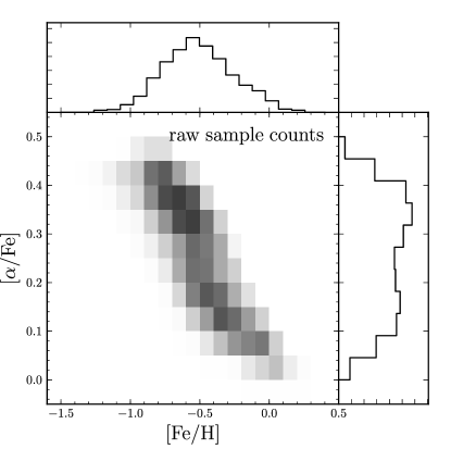
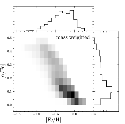
Figure 1.— Distribution of G-type dwarfs in the SDSS/SEGUE spectroscopic sample in the $[\mathrm{Fe/H}]$,$[\alpha\mathrm{/Fe}]$ elemental-abundance plane. The left panel shows the raw number counts, while the right panel shows mass-weighted number counts that are corrected for spectroscopic selection effects and converted into total stellar surface-mass densities at the Solar radius using the stellar population modeling described in Appendix A. Pixels span 0.1 dex in $[\mathrm{Fe/H}]$ and 0.05 dex in $[\alpha\mathrm{/Fe}]$, which is larger than in the equivalent Figure in Lee et al. (2011), as the spatial number-density fitting used as part of the mass-weighting demands larger bins. The mass weighting shows that the prominent bi-modality seen in the raw number counts (left, cf. Lee et al., 2011) is mostly a consequence of the uneven spectroscopic sampling of the underlying stellar populations. The remaining hint of $[\alpha\mathrm{/Fe}]$ bi-modality seen in the right panel is a natural consequence of the enrichment physics, i.e., SN Ia enrichment delays, even for a perfectly uniform (enrichment) age distribution (e.g., Schönrich & Binney, 2009a).

$\bullet$ Conceptually the right approach seems to be to define sub-samples by a property that may correlate with disk structure but is formally independent of it, such as stellar age or stellar abundances. Such ‘tags’ are properties that do not change along the orbit of the star, nor do they change if a star changes its orbit due to a minor merger or radial migration (Freeman & Bland-Hawthorne, 2002); in this sense, tagging stellar populations by elemental abundances is even better than using the best structural or dynamical tags available: integrals of motion, or orbital actions. With such sub-samples, one can then ask whether their respective disk structures suggest distinct thin and thick disks. This approach has been re-advocated in recent studies (Navarro et al., 2011; Lee et al., 2011), drawing on the seemingly bi-modal distribution of stars in the $[\alpha\mathrm{/Fe}]$ - $[\mathrm{Fe/H}]$ plane of elemental abundances; however, these studies did not account for selection effects and volume corrections.

Believing that the last approach is the conceptually correct one, we derive in this paper for the first time a scale-height distribution of the stellar mass at the Solar radius in the Galaxy to see whether this distribution shows any evidence of bi-modality. This requires two steps: first, one needs to associate a vertical scale-height with any given star. Our recent analysis (B11) showed that sub-populations of stars of a given $[\alpha\mathrm{/Fe}]$ and $[\mathrm{Fe/H}]$ are well described by a single exponential in their vertical profile, making ($[\alpha\mathrm{/Fe}]$,$[\mathrm{Fe/H}]$) a suitable tag for each star that uniquely determines the scale-height of its sub-population. Second, one needs to determine what the (surface) mass fraction of stars is in this $[\alpha\mathrm{/Fe}]$– $[\mathrm{Fe/H}]$ sub-population. As such samples can only be defined through spectroscopic surveys, this in turn requires proper accounting for the spectroscopic survey selection function (B11), and an estimate of the stellar mass fraction that the spectroscopically targeted stars represent of the entire population at this elemental abundance.

We work out this last step in this paper ($\mathsection$ 2), and on that basis derive the distribution of stellar surface-mass density-weighted distribution of stellar scale heights at $R_{0}$, $\Sigma_{R_{0}}(h_{z})$ ($\mathsection$ 2). Surprisingly, we find a smooth, exponentially-declining surface-mass-density spectrum as a function of scale height between $\approx$ 200 and 1000 pc. This mass spectrum shows no gaps, excess, or hints of bi-modality at large scale heights, leading us to conclude that the Milky Way has no distinct thick disk. We discuss implications, and explain how this relates to recent work that arrived at qualitatively different conclusions, in $\mathsection$ 3.

2. The mass-weighted scale height distribution of disk stars in the Milky Way

Recently, we have performed (in B11) number-density fits to sub-populations of stars defined as narrow boxes in the elemental-abundance plane spanned by metallicity $[\mathrm{Fe/H}]$ and $\alpha$-enhancement $[\alpha\mathrm{/Fe}]$, based on G-dwarf spectra and star counts from SDSS/SEGUE (Abazajian et al. 2009; Yanny et al. 2009; SEGUE elemental-abundance uncertainties are 0.2 dex in $[\mathrm{Fe/H}]$ and 0.1 dex in $[\alpha\mathrm{/Fe}]$). G-type dwarfs are the most luminous tracers whose main-sequence lifetime is larger than the expected disk age at basically all metallicities. We refer the reader to B11 for a discussion of the data set and for a detailed description and discussion of these fits, accounting for the volume correction of the spectroscopic survey. B11 show that each mono-abundance sub-population has a simple density structure that can be described by an exponential profile both in Galactocentric radius $R$ and vertical height $z$. The inferred scale heights for different mono-abundance sub-populations vary with $[\alpha\mathrm{/Fe}]$ and $[\mathrm{Fe/H}]$, increasing smoothly from about 200 pc to about 1200 pc when going from populations with near-solar abundances to populations that are more metal-poor and enhanced in $\alpha$ elements.

These results were derived from the spectroscopic SEGUE G-dwarf sample, whose face-value distribution in the $[\mathrm{Fe/H}]$–$[\alpha\mathrm{/Fe}]$ plane is suggestive of two distinct populations definable in this elemental-abundance space, because there is a peak near solar abundances and one at metal-poor and $\alpha$-enhanced abundances (see Lee et al. 2011, B11, and the left panel of Figure 1). However, SEGUE targeted stars at high latitudes in an apparent-magnitude range $14.5\leq r\leq 20.2$ that finds G-type dwarfs at vertical heights $\gtrsim 500$ pc, significantly above the bulk of the thin-disk population (which B11 inferred to have a scale height of 250 pc). Additionally, G-type dwarfs of different metallicities have different luminosity and hence survey volumes, and the spectroscopic targeting was weighted toward the fainter end of the apparent-magnitude range and toward higher latitudes (see Yanny et al. 2009 and the discussion in Appendix A of B11). Thus, the distribution of the SEGUE sample in the $[\mathrm{Fe/H}]$–$[\alpha\mathrm{/Fe}]$ plane reflects the survey selection function more than the abundance distribution of the Milky Way stars within 1 to 2 kpc from the Sun.

To properly assess the contribution of the various mono-abundance sub-populations to the mass or surface-mass budget in the Solar neighborhood, we must convert the number of spectroscopically-observed stars in each bin to a surface-mass density at the Solar neighborhood. On the one hand, this requires incorporation of a model for the SEGUE selection function (see Appendix A of B11) and our exponential-disk fits (B11). On the other hand, this requires the use of stellar-population models that can relate the observed number of G-type dwarfs to the total mass of the stellar population, given the metallicity of the sub-population and an assumed star formation history for it. This is described in detail in Appendix A.

Briefly, for G-type dwarfs in a given ($[\mathrm{Fe/H}]$,$[\alpha\mathrm{/Fe}]$) bin we calculate their total number per square pc (integrated over vertical height) by adjusting the normalization of the number-density profile such that after running it through our model for the SEGUE selection function it predicts the observed number of stars in each bin. Then we relate the number density of G-type dwarfs to the total stellar surface-mass density by multiplying the number density by the average mass of a G-type dwarf—calculated using Padova isochrones (Marigo et al., 2008)—and dividing it by the fraction of the mass in a stellar population in G-type dwarfs (calculated using the same isochrones and assuming a lognormal Chabrier (2001) initial mass function). At a given abundance, this fraction of course depends on the age of the population, and here is calculated by marginalizing over a flat age distribution between 0.5 and 10 Gyr for each bin. However, averaging only over older ages for $\alpha$-enhanced stars would be appropriate, as $\alpha$-enhanced stars likely represent the oldest part of the disk. As we show in Appendix A, this gives similar results, with a slightly steeper decline in $\Sigma(R_{0})$ with $h_{z}$. We calculate uncertainties on the surface-mass densities by varying the density-parameters according to the posterior probability distribution for the parameters in B11. These uncertainties do not include systematic uncertainties due to the use of the stellar isochrones. This procedure results in an estimate of the stellar surface-mass density contribution at the Solar radius for any abundance-selected sub-population, which in turn has a vertical scale height associated with it. The relative total stellar surface-mass densities of different mono-abundance bins are not affected by assuming a different initial mass function (IMF), although assuming a different IMF can systematically shift all surface-mass densities by a few percent (see below).

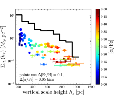
Figure 2.— Distribution of stellar surface-mass density at the Solar radius $\Sigma_{R_{0}}(h_{z})$ as a function of vertical scale height $h_{z}$. The thick black histogram shows the total stellar surface-mass density in bins in $h_{z}$, calculated by summing the total stellar masses of sub-populations in bins in $[\alpha\mathrm{/Fe}]$ and $[\mathrm{Fe/H}]$. The stellar surface-mass densities of the individual elemental-abundance bins in $[\mathrm{Fe/H}]$ and $[\alpha\mathrm{/Fe}]$ are shown as dots, with values for $\Sigma_{R_{0}}([\mathrm{Fe/H}],[\alpha\mathrm{/Fe}])$ on the $y$-axis. The points are color-coded by the value of $[\alpha\mathrm{/Fe}]$ in each bin and the size of the points is proportional to the square root of the number of data points that the density fits are based on. Some of the errorbars are smaller than the points. Elemental abundance bins have a width of 0.1 in $[\mathrm{Fe/H}]$ and 0.05 in $[\alpha\mathrm{/Fe}]$.

The results from this mass estimation are shown in Figures 1 and 2. The left panel of Figure 1 is simply a more coarsely binned version of the unweighted SEGUE G-dwarf sample abundance distribution, which shows two distinct maxima, one considerably more metal poor and $\alpha$-enhanced than the other, seemingly reflecting a chemically-distinct thick-disk component. It is important to note that the marginalized $[\mathrm{Fe/H}]$ metallicity distribution (left panel, top) shows no hint of any bi-modality. There is distinct bi-modality in the marginalized $[\alpha\mathrm{/Fe}]$ distribution, but Schönrich & Binney (2009a) already showed that even for a smooth age distribution such bi-modality arises, simply separating stars that formed before and after enrichment by SN Ia became important. The right panel of Figure 1 shows the stellar surface-mass density at the solar radius $R_{0}$ in each elemental-abundance bin, corrected for selection effects due to the spectroscopic SEGUE selection as described above. It represents the properly mass-weighted, underlying distribution of disk stars in the elemental-abundance space spanned by $[\mathrm{Fe/H}]$ and $[\alpha\mathrm{/Fe}]$, and dramatically differs from the raw sample distribution in the left panel: it does not have the strong bi-modality apparent in the raw SDSS/SEGUE number distribution. It also shows no hint of a bi-modal $[\mathrm{Fe/H}]$ metallicity distribution and the remaining hint of $[\alpha\mathrm{/Fe}]$ bi-modality is explained as in the left panel.

The right panel of Figure 1 now provides the relevant weights of each mono-abundance bin to a surface-mass-weighted distribution of disk scale heights. The colored symbols in Figure 2 show exactly these surface-mass density contributions for all these mono-abundance bins in $[\mathrm{Fe/H}]$ and $[\alpha\mathrm{/Fe}]$ (with widths 0.1 in $[\mathrm{Fe/H}]$ and 0.05 in $[\alpha\mathrm{/Fe}]$) versus the scale height of those sub-population from B11, color-coded by their $[\alpha\mathrm{/Fe}]$ enhancement. We then sum the surface-mass contributions $\Sigma_{R_{0}}(h_{z}|[\mathrm{Fe/H}],[\alpha\mathrm{/Fe}])$ of sub-populations ($[\mathrm{Fe/H}]$,$[\alpha\mathrm{/Fe}]$) into bins in scale height. This results in the thick black histogram, which represents $\Sigma_{R_{0}}(h_{z})$, or more simply $p(h_{z})$, the surface-mass weighted distribution of vertical scale heights in the Solar neighborhood (which we will refer to in the remainder simply as the ‘scale-height distribution’). That is, for any random stellar-mass element this function gives the probability density for the scale height of the structural component to which it belongs. This is the function we set out to construct in order to examine whether it makes sense to think of distinct thin and thick disk components in the Milky Way. Remarkably, we find that the scale-height distribution simply decreases quite smoothly towards larger scale heights, with an approximately exponential relation between surface-mass density and scale height $\Sigma(R_{0})\propto\exp(-h_{z})$. The scale height distribution does not show any gaps, excesses, or hints of bi-modality, beyond this simple relation.

By combining all of the stellar surface-mass density estimates we can precisely measure the total visible stellar surface-mass density at the Solar radius. We find $\Sigma^{{}^{*}}_{R_{0}}=30\pm 1\ M_{\odot}$ pc^-2. This is similar to the estimate of Flynn et al. (2006), who report $\Sigma^{{}^{*}}_{R_{0}}=29\ M_{\odot}$ pc^-2. This estimate depends slightly on the assummed IMF. Using the exponential IMF (IMF3) of Chabrier (2001) gives $\Sigma^{{}^{*}}_{R_{0}}=29.5\ M_{\odot}$ pc^-2; the IMF from Chabrier (2003) gives $\Sigma^{{}^{*}}_{R_{0}}=29\ M_{\odot}$ pc^-2; and a Kroupa (2003) IMF gives $\Sigma^{{}^{*}}_{R_{0}}=32\ M_{\odot}$ pc^-2.

3. Discussion

Figure 1 shows that properly correcting for the spectroscopic sampling of the underlying stellar sub-populations is crucial in assessing the elemental-abundance distribution at $R_{0}$ of spectroscopically selected samples of stars. The abundance distribution without this correction is heavily influenced by the survey-specific spatial and mass sampling of the underlying stellar population—both of which act to make the metal-poor and $\alpha$-enhanced sub-populations more prominent in the high-latitude and color-selected SEGUE sample—which leads to a spuriously enhanced bi-modality in elemental-abundance space. The mass-weighted metallicity distribution in Figure 1 has no bi-modality. The mass-weighted $[\alpha\mathrm{/Fe}]$-distribution in the same Figure has only a hint of a bi-modality, as is expected in standard smooth star formation and enrichment scenarios (Schönrich & Binney, 2009a), and reflects enrichment physics and not galaxy evolution.

Improper weighting of the distribution of structural parameters can again lead to spurious bi-modal signatures. Figure 5 in B11 shows the location of chemically-defined sub-populations in the space of the structural parameters (radial scale length, vertical scale height). This scatterplot, based on equal-area bins in ($[\mathrm{Fe/H}]$,$[\alpha\mathrm{/Fe}]$), gives undue prominence to the low-$[\mathrm{Fe/H}]$, high-$[\alpha\mathrm{/Fe}]$ (with respect to solar abundances) bins, as many of them only contribute a negligible amount to the total stellar mass. Here, Figure 2 shows that the proper mass-weighting of the ($[\mathrm{Fe/H}]$,$[\alpha\mathrm{/Fe}]$) sub-populations gives a vertical-scale-height distribution that is smooth and monotonically declining between thinner disk component scale heights of 200 pc and thicker components’ scale heights of $\approx 1200$ pc, with no gaps or excesses beyond the smooth, approximately exponential distribution. B11 found that each elemental-abundance bin was preferentially fit by a single exponential rather than by two disk components, such that the smooth scale-height distribution in Figure 2 is not merely the result of the smoothing out of an intrinsically bi-modal distribution by elemental-abundance errors (which are small for the SEGUE sample, see $\mathsection$ 2) or overlapping abundance distributions of distinct “thin” and “thick” disks; if either of these were the case B11 should have detected two components in the abundance bins with single-exponential scale heights in the range of approximately 400 to 600 pc. The large uncertainties on the radial scale lengths of the chemically-defined mono-abundance sub-populations in B11 complicate a similar assessment of the radial structure of the disk, but this has no bearing on the analysis of the vertical structure. Upcoming surveys such as APOGEE (Eisenstein et al., 2012) or HERMES/GALAH (Freeman et al., 2010) that will sample stellar populations in the plane of the Milky Way will be able to study the radial structure in more detail.

Thus, stars in the Solar neighborhood have a smoothly decreasing probability of belonging to structural components with increasing scale heights. This implies that the thicker disk component in the Milky Way is simply the tail of a continuous and monotonic scale-height distribution. This has been suggested before (e.g., Norris, 1987; Schönrich & Binney, 2009b), but never directly measured as we do here. As such, there is no distinct thick-disk component in our Galaxy.

Together with the findings in B11 that the thicker and older components of the Galactic disk have a shorter radial scale lengths than the thinner and younger components this qualitatively points toward a continuous internal mechanism such as radial migration or turbulent disk evolution being predominantly responsible for the thickening of the disk, rather than an external merger or heating event. However, a rigorous comparison with models, where thick stellar-disk components arise from one or a few distinct events triggered, e.g., by satellite infall, is needed to see whether the present data are indeed inconsistent with the results presented here. Formation age of stars may serve as a sensible marker in simulations to associate individual stars with a ‘parent sub-population’ whose scale height can be determined. In this context, it is worth noting that combined data from APOGEE and Kepler will soon provide ages for a large number of stars through asteroseismology (e.g., Gilliland et al., 2010), which could help in mapping mono-age populations into the mono-abundance populations studied here.

The proper selection function analysis and subsequent conversion to stellar mass densities can of course be used in the future to look with proper mass weighting at other disk diagnostics beyond the spatial distribution, such as the orbital eccentricity or vertical motions, which has not been done correctly (e.g., Dierickx et al., 2010; Wilson et al., 2011).

Our results that show that the Milky Way has no distinct thick-disk component might appear to be at odds with observations of external edge-on galaxies, where “thick disk” components are found to be universal (e.g., Yoachim & Dalcanton, 2006). However, those decompositions are restricted to luminosity-weighted geometric decompositions and suffer from the uncertain influence of dust in the mid-plane of the galaxies; they cannot isolate components based on elemental abundances; and they only perform discrete two-component fits, which naturally prefers two components over a single exponential component, even though the underlying scale-height distribution might be more complicated, as shown in this paper. The findings from external galaxies might be more correctly interpreted as proving the universality of thicker disk components rather than that of “thick disks”.

Appendix A The surface-mass density in a mono-abundance sub-population

In practice, we calculate the surface-mass density contribution at the Solar radius from each mono-abundance sub-component, defined as a box in the $[\mathrm{Fe/H}]$–$[\alpha\mathrm{/Fe}]$ plane, by first converting the observed number counts into a ‘number column density’ ($N(R_{0})$ in the notation of B11; units stars pc^-2) and then converting this number density into a total stellar surface-mass density using stellar-population models. This involves estimating the mean (individual) stellar masses of the stars we have in the sample, and estimating which fraction of their total stellar population at that abundance that mass range constitutes.

When performing the stellar number-density fits in B11 we did not fit for the normalization of the density. However, we can calculate this normalization by adjusting it such that it predicts the observed number of stars when we run the density model through the observational selection function. Thus, we calculate the predicted number of stars for a density normalized to have unit surface-mass density (in stars pc^-2); the correct normalization constant is then the total number of observed stars divided by the predicted number of stars for unit surface-mass density. We calculate the uncertainty in this number by performing this procedure for each of the samples from the posterior distribution for the number-density parameters, obtained in B11 to estimate the uncertainties in the best-fit number-density parameters. This gives for each abundance bin a number $N(R_{0};[\mathrm{Fe/H}],[\alpha\mathrm{/Fe}])\pm\sigma_{N;[\mathrm{Fe/H}],[\alpha\mathrm{/Fe}]}$ that represents the total number of stars per square pc in this $[\mathrm{Fe/H}]$–$[\alpha\mathrm{/Fe}]$ bin at the Solar radius.

In order to turn this number density $N(R_{0};[\mathrm{Fe/H}],[\alpha\mathrm{/Fe}])$ into a stellar mass we use stellar isochrones in the SDSS photometric system (Girardi et al., 2004; Marigo et al., 2008; Girardi et al., 2010) to model the mass $M(g-r,\tau,[\mathrm{Fe/H}])$ as a function of color $g-r$, age $\tau$, and metallicity $[\mathrm{Fe/H}]$. The isochrones all assume $[\alpha\mathrm{/Fe}]=0$. A lognormal Chabrier (2001) mass function $\phi(M)$ is used to weight the contribution of various masses to the stellar population’s mass (i.e., the mass function provides the measure in mass space). Assuming different forms for the IMF systematically changes the stellar surface-mass densities by a few percent independent of metallicity.

The total stellar mass is related to the number of G-type dwarfs approximately as

$$\mathrm{stellar\ mass\ in\ a\ [\mathrm{Fe/H}]-[\alpha\mathrm{/Fe}]\ bin}=N(R_{0};[\mathrm{Fe/H}],[\alpha\mathrm{/Fe}])\,\langle M_{\mathrm{G}}\rangle([\mathrm{Fe/H}])\,\omega^{-1}([\mathrm{Fe/H}])\,,$$ (A1)

where $\langle M_{\mathrm{G}}\rangle$($[\mathrm{Fe/H}]$) is the average mass of a G-type dwarf in the $0.45\leq g-r\leq 0.58$ color range and $\omega$($[\mathrm{Fe/H}]$) is the ratio of a stellar population’s mass in G-type dwarfs to the total mass in the population. We calculate both $\langle M_{\mathrm{G}}\rangle$($[\mathrm{Fe/H}]$) and $\omega$($[\mathrm{Fe/H}]$) using the stellar isochrones and assuming a lognormal Chabrier (2001) initial mass function.

We calculate the mass in G-type dwarfs of a stellar population as

$$M_{\mathrm{G,total}}([\mathrm{Fe/H}])=\int_{0.45}^{0.58}\mathrm{d}(g-r)\int_{\tau_{\mathrm{min}}}^{\tau_{\mathrm{max}}}\mathrm{d}\tau\int\mathrm{d}M\,\phi(M)\,M(g-r,\tau,[\mathrm{Fe/H}])\,,$$ (A2)

where we thus use a flat prior in age and we only use the dwarf part of the isochrone. The total stellar mass of a stellar population is given by a similar expression, but without the color restriction. In what follows we use ($\tau_{\mathrm{min}},\tau_{\mathrm{max}}$) = (0.5,10) Gyr for all abundance bins. As $[\alpha\mathrm{/Fe}]$ is a relative age indicator (see discussion in B11) with populations with $[\alpha\mathrm{/Fe}]\gtrsim 0.25$ probably $\gtrsim 7$ Gyr old an $[\alpha\mathrm{/Fe}]$-dependent age distribution would be more appropriate, although the exact form it should take is hard to establish. We also used ($\tau_{\mathrm{min}},\tau_{\mathrm{max}}$) = (1,8) Gyr for $[\alpha\mathrm{/Fe}]<0.25$ and ($\tau_{\mathrm{min}},\tau_{\mathrm{max}}$) = (7,10) Gyr for $[\alpha\mathrm{/Fe}]>025$ and found no significant difference in the inferred stellar masses for all of the abundance bins. $\omega([\mathrm{Fe/H}])$ is then the ratio of the stellar mass in G-type dwarfs to the total stellar mass. The ratio $\omega([\mathrm{Fe/H}])$ is approximately given by

$$\omega([\mathrm{Fe/H}])\approx 0.0425+0.0198\,[\mathrm{Fe/H}]\,+0.0057\,[\mathrm{Fe/H}]^{2}\,,$$ (A3)

between -1.5 $<[\mathrm{Fe/H}]<0.3$.

We calculate the average mass of a G-type dwarf in our color range using a similar procedure. We calculate the average mass by marginalizing over the same age distribution, but without weighting by the mass function as the color dependence of the mass function is very limited over this narrow color range and the distribution of the SEGUE G-dwarf sample is uniform in color $g-r$. The average mass is thus calculated as

$$\langle M_{\mathrm{G}}\rangle([\mathrm{Fe/H}])=\int_{0.45}^{0.58}\mathrm{d}(g-r)\int_{\tau_{\mathrm{min}}}^{\tau_{\mathrm{max}}}\mathrm{d}\tau\,M(g-r,\tau,[\mathrm{Fe/H}])\,;$$ (A4)

this is approximately given by

$$\langle M_{\mathrm{G}}/M_{\odot}\rangle([\mathrm{Fe/H}])\approx 0.956+0.205\,[\mathrm{Fe/H}]\ +0.051\,[\mathrm{Fe/H}]^{2}\,,$$ (A5)

again between -1.5 $<[\mathrm{Fe/H}]<0.3$.

The average mass $\langle M_{\mathrm{G}}\rangle([\mathrm{Fe/H}])$ of a G-type dwarf as a function of $[\mathrm{Fe/H}]$ only changes by about 20 percent when going from metal-poor to metal-rich stars, with more metal-poor stars having smaller masses. The fractional contribution to the mass budget of G-type dwarfs $\omega$($[\mathrm{Fe/H}]$) decreases from 5 percent for metal-rich stars to approximately 3 percent for metal-poor stars. Thus, these mass-correction factors are not the main drivers for the structure in Figure 2.

References

- Abadi et al. (2003) Abadi, M. G., Navarro, J. F., Steinmetz, M., & Eke, V. R. 2003, ApJ, 591, 499
- Abazajian et al. (2009) Abazajian, K. N., Adelman-McCarthy, J. K., Agũeros, M. A., et al. 2009, ApJS, 182, 543
- Bensby et al. (2005) Bensby, T., Feltzing, S., Lundström, I., & Ilyin, I. 2005, A&A, 433, 185
- Bensby et al. (2011) Bensby, T., Alves-Brito, A., Oey, M. S., Yong, D., & Meléndez, J. 2011, ApJ, 735, L46
- Bovy et al. (2011) Bovy, J., Rix, H.-W., Liu, C., Hogg, D. W., Beers, T. C., & Lee, Y. S. 2011, ApJ, submitted, arXiv:1111.1724 [astro-ph.GA] (B11)
- Bournaud et al. (2009) Bournaud, F., Elmegreen, B. G., & Martig, M. 2009, ApJ, 707, L1
- Brook et al. (2004) Brook, C. B., Kawata, D., Gibson, B. K., & Freeman, K. C. ApJ, 612, 894
- Burstein (1979) Burstein, D. 1979, ApJ, 234, 829
- Chabrier (2001) Chabrier, G. 2001, ApJ, 554, 1274
- Chabrier (2003) Chabrier, G. 2003, PASP, 115, 763
- Chiba & Beers (2000) Chiba, M. & Beers, T. C. 2000, AJ, 119, 2843
- Dierickx et al. (2010) Dierickx, M., Klement, R., Rix, H.-W., & Liu, C. 2010, ApJ, 725, L186
- Eisenstein et al. (2012) Eisenstein, D. J., Weinberg, D. H., Agol, E., et al. 2012, AJ, 142, 72
- Feltzing et al. (2003) Feltzing, S., Bensby, T., & Lundström, I. 2003, A&A, 397, 1
- Flynn et al. (2006) Flynn, C., Holmberg, J., Portinari, L., Fuchs, B., & Jahreiß, H. 2006, MNRAS, 372, 1149
- Förster Schreiber et al. (2009) Förster Schreiber, N. M., Genzel, R., Bouché, N., et al. 2009, ApJ, 706, 1364
- Freeman & Bland-Hawthorne (2002) Freeman, K. & Bland-Hawthorn, J. 2002, ARA&A, 40, 487
- Freeman et al. (2010) Freeman, K., Bland-Hawthorn, J., & Barden, S. 2010, AAO Newsletter, 117, 9
- Fuhrmann (1998) Fuhrmann, K. 1998, A&A, 338, 161
- Gilliland et al. (2010) Gilliland, R. L., Brown, T. M., Christensen-Dalsgaard, J., et al. 2010, PASP, 122, 131
- Gilmore & Reid (1983) Gilmore, G. & Reid, N. 1983, MNRAS, 202, 1025
- Girardi et al. (2004) Girardi, L., Grebel, E. K., Odenkirchen, M., & Chiosi, C. 2004, A&A, 422, 205
- Girardi et al. (2010) Girardi, L., Williams, B. F., Gilbert, K. M.,et al. 2010, ApJ, 724, 1030
- Jurić et al. (2008) Jurić, M., Ivezić, Ž., Brooks, A., et al. 2008, 673, 864
- Kazantzidis et al. (2008) Kazantzidis, S., Bullock, J. S., Zentner, A. R., Kravtsov, A. V., Moustakas, L. A. 2008, ApJ, 688, 254
- Kroupa (2003) Kroupa, P. 2003, MNRAS, 322, 231
- Lee et al. (2011) Lee, Y. S., Beers, T. C, An, D., et al. 2011, ApJ, 738, 187
- Marigo et al. (2008) Marigo, P., Girardi, L., Bressan, A., Groenewegen, M. A. T., Silva, L., & Granato, G. L. 2008, A&A, 482, 883
- Navarro et al. (2011) Navarro, J. F., Abadi, M. G., Venn, K. A., Freeman, K. C., & Anguiano, B. 2011, MNRAS, 412, 1203
- Nemec & Nemec (1991) Nemec, J. & Nemec, A. F. L. 1991, PASP, 103, 95
- Nemec & Nemec (1993) Nemec, J. & Nemec, A. F. L. 1993, AJ, 105, 1455
- Norris (1987) Norris, J. 1987, ApJ, 314, L39
- Norris (1999) Norris, J. E. 1999, Ap&SS, 165, 213
- Prochaska et al. (2000) Prochaska, J. X., Naumov, S. O., Carney, B. W., McWilliam, A., & Wolfe, A. M. 2000, AJ, 120, 2513
- Quinn et al. (1993) Quinn, P. J., Hernquist, L., & Fullagar, D. P. 1993, ApJ, 403, 74
- Reid & Majewski (1993) Reid, N. & Majewski, S. R. 1993, ApJ, 409, 635
- Ryan & Norris (1993) Ryan, S. G. & Norris, J. E. 1993, in Galaxy Evolution. The Milky Way Perspective. ed. S. R. Majewski (Astronomical Society of the Pacific), 49, 103
- Sales et al. (2009) Sales, L. V., Helmi, A., Abadi, M. G., et al. 2009, MNRAS, 400, L61
- Schönrich & Binney (2009a) Schönrich, R. & Binney, J. J. 2009a, MNRAS, 396, 203
- Schönrich & Binney (2009b) Schönrich, R. & Binney, J. J. 2009b, MNRAS, 399, 1145
- Sellwood & Binney (2002) Sellwood, J. A. & Binney, J.J. 2002, MNRAS, 336, 785
- Tsikoudi (1979) Tsikoudi, V. 1979, ApJ, 234, 842
- van der Kruit & Searle (1981) van der Kruit, P. C. & Searle, L. 1981, A&A, 95, 105
- Wilson et al. (2011) Wilson, M. L., Helmi, A.; Morrison, H. L., et al. 2011, MNRAS, 413, 2235
- Yanny et al. (2009) Yanny, B., Rockosi, C., Newberg, H. J., et al. 2009, AJ, 137, 4377
- Yoachim & Dalcanton (2006) Yoachim, P. & Dalcanton, J. J. 2006, AJ, 131, 226