The ELM Survey. III. A Successful Targeted Survey for Extremely Low Mass White Dwarfs

Abstract

Extremely low mass (ELM) white dwarfs (WDs) with masses $<0.25$ $M_{\odot}$ are rare objects that result from compact binary evolution. Here, we present a targeted spectroscopic survey of ELM WD candidates selected by color. The survey is 71% complete and has uncovered 18 new ELM WDs. Of the 7 ELM WDs with follow-up observations, 6 are short-period binaries and 4 have merger times less than 5 Gyr. The most intriguing object, J1741+6526, likely has either a pulsar companion or a massive WD companion making the system a possible supernova Type Ia or .Ia progenitor. The overall ELM Survey has now identified 19 double degenerate binaries with $<$10 Gyr merger times. The significant absence of short orbital period ELM WDs at cool temperatures suggests that common envelope evolution creates ELM WDs directly in short period systems. At least one-third of the merging systems are halo objects, thus ELM WD binaries continue to form and merge in both the disk and the halo.

1. INTRODUCTION

Extremely low-mass (ELM) WDs with masses $<$0.25 $M_{\odot}$ are created when the progenitor stars lose so much mass during their evolution that they never reach helium burning. Binary evolution is considered the most likely origin for low-mass WDs (e.g. Marsh et al., 1995), making ELM WDs the signposts for the type of compact systems that are strong gravitational wave sources. In Paper I of this series (Brown et al., 2010) we presented the first complete, well-defined sample of ELM WDs fortuitously targeted by the Hypervelocity Star Survey (Brown et al., 2005, 2006, 2009). In paper II of this series (Kilic et al., 2011a) we characterized other ELM WDs identified in the Sloan Digital Sky Survey (SDSS) Data Release 4 (Eisenstein et al., 2006). In both programs ELM WDs exist in $\leq 1$ day orbital period binary systems, with an estimated merger rate comparable to the rate of underluminous supernovae (Brown et al., 2011a).

Here we present the results of the first targeted survey for new ELM WDs. Our approach is to select high-probability ELM WD candidates from a well-defined region of color and apparent magnitude, and then obtain spectroscopy for the objects from that selection region. The spectroscopic survey is presently 71% complete and contains 21 ELM WDs defined by $5.0<\log{g}<7.0$ dex ($g$ in cm s^-2). Three of the ELM WDs were previously identified (Kilic et al., 2009; Brown et al., 2010) and 18 are new discoveries. We have obtained follow-up spectroscopy for 7 of the new ELM WDs, and calculate orbital solutions for the 6 with significant velocity variability. Four of these new ELM WD systems have gravitational wave merger times less than 5 Gyr. The most interesting object, J1741+6526, has a minimum companion mass of 1.1 $M_{\odot}$. Thus J1741+6526 is most likely a pulsar binary, or, if the orbit is edge-on, possibly a supernova Type Ia or .Ia progenitor (Bildsten et al., 2007). It will begin mass transfer in $<$170 Myr.

Our targeted ELM survey will yield a clean, non-kinematically selected sample of WDs. Once completed, we can use our sample to constrain the space density, period distribution, and merger rate of ELM WDs in double degenerate systems. SDSS, on the other hand, has not found large numbers of ELM WDs because they have not targeted them; existing SDSS WD spectroscopy comes from different target selection programs observed with different completenesses (Eisenstein et al., 2006). In a stellar evolution context, our survey complements studies of WD binaries with main sequence companions (Zorotovic et al., 2011; Nebot Gómez-Morán et al., 2011). Because of ELM WDs’ low surface gravities $\log{g}\sim 6$ and small $\simeq$1 $R_{\odot}$ orbital separations, a growing number of systems exhibit some combination of tidal distortion, relativistic beaming, reflection effects, and eclipses (e.g. Brown et al., 2011b; Kilic et al., 2011c; Parsons et al., 2011; Pyrzas et al., 2011; Steinfadt et al., 2010; Vennes et al., 2011). We expect that on-going photometric follow-up will provide improved constraints on the nature and orbital inclination of our new ELM WD binary systems.

We organize this paper as follows. In Section 2 we discuss our new survey design, observations, and data analysis. In Section 3 we present the orbital solutions for six new ELM WD binaries. In Section 4 we discuss the overall properties of the ELM WD sample and highlight correlations between temperature, orbital period, and secondary mass. We conclude in Section 5.

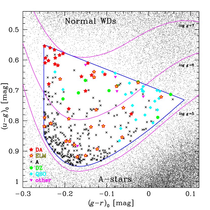
Figure 1.— Color-color diagram showing our ELM Survey selection region (blue bounded region) in the context of SDSS star counts (black dots). The ELM Survey selection targets a region of color space that contains $5<\log{g}<7$ dex hydrogen atmosphere WDs (magenta solid lines) and avoids known concentrations of A-type stars and normal WDs. Symbols indicate the spectroscopic identification of ELM Survey targets: red stars are the DA WDs, red stars with yellow centers are the ELM WDs, black x’s are normal A-type stars, green circles are DZ WDs, cyan diamonds are quasars, and magenta triangles are other miscellaneous objects.

2. DATA AND ANALYSIS

2.1. ELM Survey Design

The ELM Survey is a spectroscopic survey of $15<g_{0}<20$ low mass WD candidates selected by color. We use de-reddened, uber-calibrated point spread function magnitudes from SDSS Data Release 7 (Abazajian et al., 2009). Our color selection strategy, illustrated in Figure 1, is constructed as follows.

First, we target objects with colors consistent with the effective temperatures of luminous ELM WDs. Updated Panei et al. (2007) evolutionary tracks for He-core WDs indicate that 0.17 $M_{\odot}$ WDs spend $\simeq$1 Gyr with luminosities of $8<M_{g}<9$ mag at temperatures $\sim$10,000 K. Serenelli et al. (2001) tracks give similar results. Thus we target $-0.25<(g-r)_{0}<0.1$. Second, we target objects with $(u-g)_{0}$ colors consistent with the $5<\log{g}<7$ surface gravities of ELM WDs. To make this color selection, we use a polynomial fit to the synthetic photometry of DA WD hydrogen atmosphere models (Koester, 2008),

$$(u-g)_{0} < 0.83-1.074(g-r)_{0}-1.4939(g-r)_{0}^{2}$$ (1)

$$+0.8156(g-r)_{0}^{3}+33.42316(g-r)_{0}^{4}$$

$$+280.88439(g-r)_{0}^{5}-492.62139(g-r)_{0}^{6}$$

$$-1993.9254(g-r)_{0}^{7}.$$

Finally, we restrict our color-selection to the most probable low mass WD candidates. We restrict our selection to those objects bluer in $(u-g)_{0}$ than the observed population of A-type stars (our zeropoint in Equation 1) and redder in $(u-g)_{0}$ than the observed population of normal DA WDs, $(u-g)_{0}>0.542(g-r)_{0}+0.685$. We exclude quasars based on their non-stellar color $(r-i)_{0}<1.8-0.1g_{0}$, a limit that becomes more restrictive at faint magnitudes where we expect greater contamination from increased photometric errors and from increased quasar number counts. Put together, this color selection strategy maximizes the contrast of ELM WDs with respect to foreground and background populations.

Our target selection identifies 505 ELM WD candidates with $15<g<20$ over $\simeq$10,000 deg² of the Sloan Data Release 7 imaging footprint. Spectra for 116 of these candidates already exist: 31 of the candidates were observed by the Hypervelocity Star survey (Brown et al., 2009), and 85 were observed by SDSS. Three of the objects with existing spectra are previously identified merging ELM WD binaries (Kilic et al., 2009; Brown et al., 2010), thus our initial expectation is that we will find about a dozen new merging ELM WD binaries in the full survey. There remain 389 candidates to observe.

2.2. Spectroscopic Observations

We obtained spectra for 245 of the ELM WD candidates in observing runs starting in 2010 September and ending in 2011 June. We observed 164 objects with $g>17$ mag at the 6.5m MMT telescope using the Blue Channel spectrograph (Schmidt et al., 1989). We operated the Blue Channel spectrograph with the 832 line mm^-1 grating in second order, providing wavelength coverage 3650 Å to 4500 Å and a spectral resolution of 1.0 - 1.2 Å, depending on whether a 1″ or 1.25″ slit was used. At $g=19$ mag we used a 400 sec exposure time to obtain a signal-to-noise (S/N) of 7 per pixel in the continuum and a $\simeq$10 km s^-1 velocity error. All objects were observed at the parallactic angle, and a comparison lamp exposure was obtained with every observation.

We observed 81 objects with $g<17$ mag in queue scheduled time at the 1.5m FLWO telescope using the FAST spectrograph (Fabricant et al., 1998). We operated FAST with the 600 line mm^-1 grating and a 2″ slit, providing wavelength coverage 3500 Å to 5500 Å and a spectral resolution of 2.3 Å. At $g=16$ mag we used a 900 sec exposure time to obtain a S/N of 10 per pixel in the continuum. A comparison lamp exposure was obtained with every observation.

We process the spectra using IRAF in the standard way. We flux-calibrate using blue spectrophotometric standards (Massey et al., 1988), and we measure radial velocities using the cross-correlation package RVSAO (Kurtz & Mink, 1998). During the course of the ELM Survey we obtained repeat observations for 7 of the newly identified ELM WDs.

2.3. Spectroscopic Identifications

Of the 361 survey targets for which we have spectroscopy: 285 (78.9%) are normal A-type stars with $\log{g}\leq 5$, likely blue horizontal branch stars or blue stragglers in the halo; 23 (6.4%) are quasars; 8 (2.2%) are DZ WDs that show strong Caii H and K lines; 5 objects labeled “other” in Figure 1 are an emission line galaxy and four featureless continuum objects; and, most relevant to this paper, 40 objects (11.1%) are probable DA WDs with $\log{g}>5$, of which 21 (5.8% of the survey) are probable ELM WDs with $5.0<\log{g}<7.0$ dex.

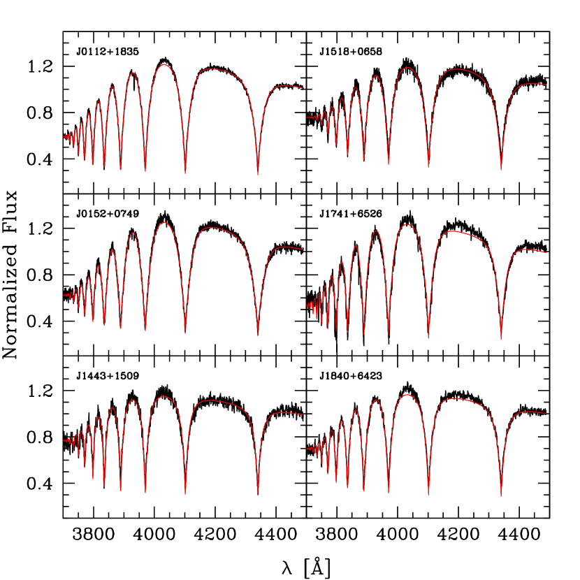
Figure 2.— Model fits (smooth red lines) overplotted on the composite observed spectra (black lines) for the six newly identified ELM WDs with significant velocity variability. We use the spectral continua to provide improved $T_{\rm eff}$ constraints.

Table 1DA White Dwarf Physical Parameters

Object	$g_{0}$	$(u-g)_{0}$	$(g-r)_{0}$	$T_{\rm eff}$	$\log g$	$M_{g}$	$d_{helio}$	Mass
	(mag)	(mag)	(mag)	(K)		(mag)	(kpc)	($M_{\odot}$)
J001622.09$-$004323.4	$19.704\pm 0.022$	$0.602\pm 0.078$	$-0.239\pm 0.040$	$11190\pm 260$	$7.40\pm 0.08$	$10.90\pm 0.14$	0.58	0.36
J011210.25+183503.7	$17.111\pm 0.015$	$0.919\pm 0.025$	$-0.170\pm 0.017$	$9690\pm 150$	$5.63\pm 0.06$	$8.00\pm 0.20$	0.66	0.16
J011726.49+251343.2	$19.300\pm 0.018$	$0.679\pm 0.055$	$-0.238\pm 0.027$	$10710\pm 190$	$7.68\pm 0.08$	$11.47\pm 0.15$	0.37	0.46
J012549.37+461920.1	$15.835\pm 0.012$	$0.778\pm 0.022$	$-0.041\pm 0.014$	$9050\pm 590$	$7.18\pm 0.12$	$11.30\pm 0.33$	0.08	0.29
J015213.77+074913.9	$18.015\pm 0.014$	$0.819\pm 0.034$	$-0.249\pm 0.021$	$10840\pm 270$	$5.80\pm 0.06$	$7.92\pm 0.10$	1.04	0.17
J021847.30+052613.7	$19.954\pm 0.027$	$0.579\pm 0.069$	$-0.204\pm 0.040$	$13510\pm 180$	$7.09\pm 0.08$	$9.91\pm 0.18$	1.02	0.30
J042154.94+830251.7	$19.789\pm 0.027$	$0.618\pm 0.126$	$-0.216\pm 0.039$	$11870\pm 200$	$7.94\pm 0.07$	$11.57\pm 0.11$	0.44	0.57
J070216.21+111009.0	$16.061\pm 0.015$	$0.764\pm 0.022$	$-0.125\pm 0.019$	$8800\pm 600$	$6.00\pm 0.12$	$9.08\pm 0.40$	0.25	0.16
J074511.56+194926.5	$16.259\pm 0.008$	$0.854\pm 0.018$	$-0.063\pm 0.020$	$8190\pm 550$	$5.70\pm 0.12$	$8.00\pm 0.20$	0.45	0.16
J074615.83+392203.1	$16.589\pm 0.018$	$0.657\pm 0.025$	$-0.130\pm 0.026$	$12130\pm 400$	$5.98\pm 0.12$	$8.44\pm 0.39$	0.43	0.17
J082904.78+370518.4	$19.242\pm 0.017$	$0.593\pm 0.048$	$-0.246\pm 0.026$	$13430\pm 230$	$7.42\pm 0.08$	$10.48\pm 0.14$	0.57	0.38
J084325.09+371551.7	$19.890\pm 0.034$	$0.702\pm 0.081$	$-0.150\pm 0.044$	$12950\pm 280$	$7.79\pm 0.08$	$11.19\pm 0.17$	0.55	0.50
J090052.04+023413.8	$17.965\pm 0.023$	$0.639\pm 0.033$	$-0.130\pm 0.029$	$8220\pm 330$	$5.78\pm 0.07$	$8.00\pm 0.20$	0.98	0.16
J091826.05+375308.7	$18.607\pm 0.017$	$0.560\pm 0.032$	$-0.235\pm 0.034$	$12060\pm 250$	$7.91\pm 0.08$	$11.53\pm 0.14$	0.26	0.56
J095353.66+410927.4	$19.589\pm 0.022$	$0.554\pm 0.053$	$-0.248\pm 0.030$	$13040\pm 490$	$7.65\pm 0.08$	$10.91\pm 0.16$	0.54	0.46
J111215.82+111745.0	$16.235\pm 0.017$	$0.820\pm 0.034$	$-0.138\pm 0.026$	$9400\pm 490$	$5.81\pm 0.12$	$8.38\pm 0.27$	0.37	0.16
J113017.45+385550.1	$19.413\pm 0.029$	$0.761\pm 0.062$	$-0.191\pm 0.045$	$12030\pm 180$	$7.17\pm 0.08$	$10.32\pm 0.12$	0.66	0.30
J113723.44+123105.9	$19.122\pm 0.031$	$0.654\pm 0.059$	$-0.160\pm 0.036$	$13000\pm 390$	$7.79\pm 0.08$	$11.19\pm 0.18$	0.39	0.50
J114303.83+361843.8	$19.678\pm 0.021$	$0.567\pm 0.057$	$-0.225\pm 0.035$	$15090\pm 190$	$7.62\pm 0.08$	$10.54\pm 0.15$	0.67	0.46
J123316.19+160204.6	$19.829\pm 0.018$	$0.809\pm 0.068$	$-0.233\pm 0.028$	$10920\pm 190$	$5.12\pm 0.07$	$8.00\pm 0.20$	2.32	0.17
J123523.78+475029.1	$19.291\pm 0.018$	$0.650\pm 0.080$	$-0.136\pm 0.024$	$10600\pm 200$	$7.68\pm 0.08$	$11.45\pm 0.13$	0.37	0.46
J144342.74+150938.6	$18.578\pm 0.017$	$0.757\pm 0.031$	$-0.060\pm 0.023$	$8810\pm 220$	$6.32\pm 0.07$	$9.67\pm 0.23$	0.61	0.17
J151826.68+065813.2	$17.456\pm 0.019$	$0.687\pm 0.026$	$-0.076\pm 0.024$	$9810\pm 320$	$6.66\pm 0.06$	$10.08\pm 0.18$	0.30	0.20
J152122.59+032607.1	$18.439\pm 0.017$	$0.794\pm 0.041$	$-0.190\pm 0.022$	$15210\pm 250$	$5.60\pm 0.08$	$8.00\pm 0.20$	1.22	0.17
J152651.57+054335.3	$18.735\pm 0.018$	$0.789\pm 0.041$	$-0.248\pm 0.028$	$10340\pm 200$	$5.64\pm 0.08$	$8.00\pm 0.20$	1.40	0.17
J153300.03+492948.3	$19.221\pm 0.021$	$0.610\pm 0.047$	$-0.247\pm 0.030$	$15830\pm 320$	$7.75\pm 0.08$	$10.68\pm 0.20$	0.51	0.49
J161431.28+191219.4	$16.187\pm 0.019$	$0.893\pm 0.025$	$-0.123\pm 0.024$	$8590\pm 540$	$5.64\pm 0.12$	$8.00\pm 0.20$	0.43	0.16
J161722.51+131018.8	$18.605\pm 0.014$	$0.868\pm 0.041$	$-0.189\pm 0.021$	$10480\pm 240$	$5.78\pm 0.08$	$8.00\pm 0.20$	1.32	0.17
J174140.49+652638.7	$18.271\pm 0.022$	$0.879\pm 0.047$	$-0.177\pm 0.030$	$9790\pm 240$	$5.19\pm 0.06$	$8.00\pm 0.20$	1.13	0.16
J184037.78+642312.3	$18.757\pm 0.014$	$0.818\pm 0.047$	$-0.108\pm 0.019$	$9140\pm 170$	$6.16\pm 0.06$	$9.25\pm 0.13$	0.80	0.17
J191311.59+372631.7	$15.430\pm 0.007$	$0.722\pm 0.016$	$+0.030\pm 0.008$	$8070\pm 630$	$7.04\pm 0.12$	$11.55\pm 0.40$	0.06	0.25
J211921.96$-$001825.8	$20.000\pm 0.021$	$0.867\pm 0.092$	$-0.197\pm 0.033$	$10360\pm 250$	$5.36\pm 0.07$	$8.00\pm 0.20$	2.51	0.17
J213513.09$-$072442.5	$19.533\pm 0.020$	$0.584\pm 0.060$	$-0.212\pm 0.030$	$11230\pm 260$	$7.30\pm 0.08$	$10.70\pm 0.16$	0.58	0.33
J221928.48+120418.6	$17.681\pm 0.017$	$0.915\pm 0.031$	$-0.150\pm 0.022$	$9700\pm 160$	$5.12\pm 0.08$	$8.00\pm 0.20$	0.86	0.16
J221936.32$-$092617.4	$19.887\pm 0.036$	$0.593\pm 0.126$	$-0.223\pm 0.053$	$14490\pm 250$	$7.83\pm 0.08$	$11.03\pm 0.12$	0.59	0.51
J222859.93+362359.6	$16.522\pm 0.011$	$0.674\pm 0.019$	$-0.025\pm 0.014$	$8840\pm 540$	$6.73\pm 0.12$	$10.63\pm 0.37$	0.15	0.20
J223630.08+223223.8	$17.004\pm 0.021$	$0.663\pm 0.028$	$-0.211\pm 0.026$	$11290\pm 50$	$6.30\pm 0.02$	$8.83\pm 0.27$	0.43	0.17
J231757.41+060252.1	$19.449\pm 0.035$	$0.647\pm 0.065$	$-0.104\pm 0.040$	$12010\pm 280$	$6.98\pm 0.08$	$10.03\pm 0.16$	0.76	0.26
J231910.03+175824.6	$19.448\pm 0.017$	$0.610\pm 0.052$	$-0.145\pm 0.024$	$13840\pm 190$	$7.19\pm 0.08$	$10.02\pm 0.14$	0.77	0.32
J233705.02+153353.6	$19.676\pm 0.022$	$0.614\pm 0.063$	$-0.224\pm 0.033$	$11700\pm 180$	$7.63\pm 0.07$	$11.11\pm 0.11$	0.52	0.45

2.4. Stellar Atmosphere Parameters

We perform stellar atmosphere model fits using an upgraded version of the code described by Allende Prieto et al. (2006) and synthetic DA WD spectra kindly provided by D. Koester. The grid of WD model atmospheres covers effective temperatures from 6000 K to 30,000 K in steps of 500 K to 2000 K, and surface gravities from $\log{g}=$ 5.0 to 9.0 in steps of 0.25 dex. The model atmospheres are calculated assuming local thermodynamic equilibrium and include both convective and radiative transport (Koester, 2008).

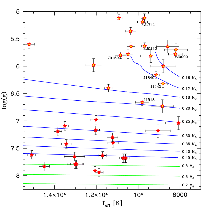
Figure 3.— Surface gravity vs. effective temperature of the observed DA WDs (solid red stars) and ELM WDs with $<$0.25 $M_{\odot}$ (stars with yellow centers) found in this survey, compared with predicted tracks for He WDs with 0.16–0.45 $M_{\odot}$ (blue lines, Panei et al., 2007) and CO WDs with 0.5–0.7 $M_{\odot}$ (green lines, Bergeron et al., 1995; Holberg & Bergeron, 2006).

We fit the full flux-calibrated spectra as well as the continuum-corrected Balmer line profiles. The spectral continuum provides improved constraints on effective temperature but exposes our fits to possible flux calibration problems – a concern for some of the objects observed in the 1.5m FAST queue, but generally not an issue for the $g>17$ mag objects observed at the MMT. When we compare best-fit solutions, the flux-calibrated and continuum-corrected parameters differ on average by $540\pm 700$ K in $T_{\rm eff}$ and $0.06\pm 0.08$ dex in $\log g$. We take these differences as our systematic error. We consider the flux-calibrated parameters more robust, because synthetic photometry of the flux-calibrated model fits provide better agreement with SDSS photometry in all five filters.

Table 1 presents the $T_{\rm eff}$ and $\log{g}$ values for the 40 DA WDs identified in the ELM Survey. For the 7 newly identified ELM WDs with multiple observations we use the flux-calibrated, summed spectra to derive $T_{\rm eff}$ and $\log{g}$, and we use the scatter of the fits to the individual spectra to derive errors. The remaining DA WDs typically have single-epoch, S/N$\simeq$8 per pixel spectra and increased statistical uncertainties in their atmospheric parameters. Two of the more massive DA WDs, J084325.09+371551.7 and J095353.66+410927.4, have SDSS stellar atmosphere measurements (Eisenstein et al., 2006) that differ from our measurements at the 1- to 2-$\sigma$ level. Figure 2 visually compares our best-fit atmosphere models with the summed spectra of the six ELM WDs with radial velocity variability. We attribute imperfect continuua fits to imperfect flux calibration, notably for J1741+6528 and J1840+6423 which were observed at high airmass.

Figure 3 plots the $T_{\rm eff}$ and $\log g$ of all 40 DA WDs in our targeted survey in relation to the improved Panei et al. (2007) tracks (see Kilic et al., 2010b) for He-core WDs with masses 0.16–0.45 $M_{\odot}$ and the Bergeron et al. (1995) tracks for normal CO-core WDs with masses 0.5–0.7 $M_{\odot}$. The gap between the 0.17 $M_{\odot}$ and 0.18 $M_{\odot}$ He-core WD tracks is linked to the threshold for thermonuclear flashes in the hydrogen shell burning phase (Panei et al., 2007). The presence of objects with $\log{g}<6$ in the gap between tracks makes precise WD mass and luminosity estimates difficult (see Kilic et al., 2011a; Vennes et al., 2011). More reliable estimates are possible for the $\log{g}>6$ WDs. Mass, luminosity, and heliocentric distance estimates are presented in Table 1.

2.5. Radial Velocities

We maximize our sensitivity to velocity variability with the following approach. We first cross-correlate the individual spectra with a high signal-to-noise WD template. We then shift the individual spectra to the rest frame, and sum them together to create a template for each object. Finally, we cross-correlate the individual spectra with the appropriate template to obtain the final velocities for each object. The average precision of our measurements is $\pm 12$ km s^-1. We verify our velocities using WD model spectra with atmospheric parameters customized for each target. The results are consistent within 10 km s^-1, which we take as our systematic velocity uncertainty. The Appendix data table presents the full set of radial velocity measurements for the 7 newly identified ELM WDs with multiple observations.

Six of the 7 newly identified ELM WDs with multiple observations display significant radial velocity variability. The ELM WD with no significant radial velocity variability is J0900+0234, however we cannot rule out whether it is a binary or not. We first observed J0900+0234 with a single exposure on 2011 March 3 and it had a heliocentric radial velocity of $64\pm 12$ km s^-1. On 2011 May 9 we re-observed the ELM WD with 9 back-to-back 2.5 min exposures and it had a mean 67 km s^-1 velocity with a $\pm 24$ km s^-1 dispersion. Although the measurement error was $\pm 13$ km s^-1, half of the observed dispersion, there was no obvious periodicity. Thus J0900+0234 shows no significant velocity variation over the observed time baselines. A future epoch of observations is required to rule out the possibility that our existing observations may have sampled the same orbital phase. Follow-up observations are planned for the other ELM WDs as well.

Figure 4.— Periodograms for the 6 newly identified ELM WDs with significant velocity variability. Some objects are well constrained, while others have multiple period aliases. In all cases the periods are $<$1 day.

Table 2Binary Orbital Parameters

Object	$P$	$K$	$\gamma$	Spec. Conjunction	Mass Function	$M_{2}$	$\tau_{\rm merge}$
	(days)	(km s-1)	(km s-1)	(days + 2455250)		($M_{\odot}$)	(Gyr)
J011210.25+183503.7	$0.14698\pm 0.00003$	$295\pm 2$	$-121\pm 1$	$259.61940\pm 0.00015$	$0.392\pm 0.007$	$\geq$ 0.62	$\leq$ 2.7
J015213.77+074913.9	$0.32288\pm 0.00014$	$217\pm 2$	$-61\pm 1$	$261.50244\pm 0.00040$	$0.341\pm 0.008$	$\geq$ 0.57	$\leq$ 22
J090052.04+023413.8	$\cdots$	$\leq 24$	$67\pm 8$	$\cdots$	$\cdots$	$\cdots$	$\cdots$
J144342.74+150938.6	$0.19053\pm 0.02402$	$307\pm 3$	$-172\pm 3$	$490.77780\pm 0.00057$	$0.569\pm 0.074$	$\geq$ 0.83	$\leq$ 4.1
J151826.68+065813.2	$0.60935\pm 0.00004$	$172\pm 2$	$-67\pm 2$	$25.98375\pm 0.00131$	$0.322\pm 0.005$	$\geq$ 0.58	$\leq$ 101
J174140.49+652638.7	$0.06111\pm 0.00001$	$508\pm 4$	$-70\pm 3$	$259.54392\pm 0.00006$	$0.830\pm 0.018$	$\geq$ 1.10	$\leq$ 0.17
J184037.78+642312.3	$0.19130\pm 0.00005$	$272\pm 2$	$-76\pm 2$	$259.43724\pm 0.00086$	$0.399\pm 0.009$	$\geq$ 0.64	$\leq$ 5.0

     

     

     

Figure 5.— Observed velocities and best-fit orbits for the 6 newly identified ELM WD binaries. Small panels plot the heliocentric radial velocities vs. observation date. Large panels plot the observations phased to the best-fit orbit (Table 2). The same vertical axis is used in all panels.

2.6. Orbital Elements

We now compute the orbital period and other orbital elements for the six ELM WDs with significant radial velocity variability. We begin by solving for the best-fit period that minimizes $\chi^{2}$ for a circular orbit. Figure 4 plots the periodograms. In some cases there are multiple period solutions because of insufficient coverage, however in all cases the periods are constrained to be $<$1 day. We estimate the period error by conservatively identifying the range of periods with $\chi^{2}\leq 2\chi^{2}_{\rm min}$, where $\chi^{2}_{\rm min}$ is the minimum $\chi^{2}$.

We compute best-fit orbital elements using the code of Kenyon & Garcia (1986), which weights each velocity measurement by its associated error. The uncertainties in the orbital elements are derived from the covariance matrix and $\chi^{2}$. To verify these uncertainty estimates, we perform a Monte Carlo analysis where we replace the measured radial velocity $v$ with $v+g\delta v$, where $\delta v$ is the error in $v$ and $g$ is a Gaussian deviate with zero mean and unit variance. For each of 10000 sets of modified radial velocities, we repeat the periodogram analysis and derive new orbital elements. We adopt the inter-quartile range in the period and orbital elements as the uncertainty. For binaries with multiple period aliases, both approaches yield similar uncertainties. When there are several equally plausible periods, the Monte Carlo analysis selects all possible periods and derives very large uncertainties. In these cases, we adopt errors from the covariance matrix for the lowest $\chi^{2}$ orbital period. We plot the best-fit orbits in Figure 5.

Table 2 presents the best-fit orbital parameters. Columns include orbital period ($P$), radial velocity semi-amplitude ($K$), systemic velocity ($\gamma$), the time of spectroscopic conjunction (the time when the object is closest to us), mass function (see Eqn. 1 below), and minimum secondary mass (assuming $i=90\arcdeg$). The systemic velocities in Table 2 are not corrected for the WDs’ gravitational redshifts, which should be subtracted from the observed velocities to find the true systemic velocities. This correction is a few km s^-1 for a 0.17 $M_{\odot}$ helium WD, comparable to the systemic velocity uncertainty.

3. RESULTS

The orbital solutions constrain the mass and thus the nature of the ELM WD binary companions, as well as the binary systems’ gravitational wave merger times. We discuss each binary in turn.

3.1. J011210.25+183503.7

The ELM WD J0112+1835 has a well-constrained orbital period of $3.5275\pm 0.0006$ hr and a radial velocity amplitude of $590\pm 4$ km s^-1. Its binary mass function is given by

$$\frac{M_{2}^{3}~{}{\rm sin}^{3}i}{(M_{1}+M_{2})^{2}}=\frac{PK^{3}}{2\pi G}=0.392\pm 0.007M_{\sun},$$ (2)

where $i$ is the orbital inclination angle, $M_{1}\simeq 0.16$ $M_{\odot}$ is the ELM WD mass inferred from Panei et al. (2007) tracks, and $M_{2}$ is the companion mass. For an edge-on orbit with $i=90\arcdeg$, Eqn. 2 provides the minimum companion mass (see Table 2). Assuming a random orbital inclination distribution, on the other hand, allows us to calculate the probability of different companion masses.

Given the observed orbital parameters, there is a 71% probability that J0112+1835’s unseen companion is a WD with $<$1.4 $M_{\odot}$ and a 14% probability that the companion is a neutron star with 1.4-3.0 $M_{\odot}$. The likelihood that the system contains a pair of WDs whose total mass exceeds the Chandrasekhar mass is 4%. If we assume the mean inclination angle for a random stellar sample, $i=60\arcdeg$, we get an estimate of the most probable companion mass. For J0112+1835, the most likely companion is a 0.85 $M_{\odot}$ WD at an orbital separation of 1.2 $R_{\odot}$.

There is no evidence for a 0.85 $M_{\odot}$ WD in the spectrum of J0112+1835, nor do we except there to be. If we pessimistically assume that the two WDs formed at the same time 100 Myr - 1 Gyr ago, we would expect the 0.85 $M_{\odot}$ companion to have $M_{g}=11-13$ mag (Bergeron et al., 1995); it would be 15 - 100 times less luminous than the 0.16 $M_{\odot}$ WD. Of course to form a short-period ELM WD binary like J0112+1835 requires two consecutive phases of common-envelope evolution in which the ELM WD is created last, giving the more massive secondary yet more time to cool and fade.

To understand the evolutionary history of J0112+1835 and our other ELM WD binaries requires assumptions about the energy balance and angular momentum balance of the common envelope phase (e.g. Nelemans et al., 2005). Kilic et al. (2010b) discuss one possible origin for a $\sim 1$ h orbital period ELM WD evolving from a system containing a 3 $M_{\odot}$ and a 1 $M_{\odot}$ star. The 3 $M_{\odot}$ star evolves off the main sequence, overflows its Roche lobe as a giant with a 0.6 $M_{\odot}$ core, forms a helium star (sdB) which does not expand after He-exhaustion in the core, and turns into a WD. The 1 $M_{\odot}$ star also overflows its Roche lobe after main-sequence evolution when its core is around 0.2 $M_{\odot}$. We can estimate orbital separations if we assume that the evolved stars exactly fill their Roche lobes. In this case, the first common-envelope phase has an orbital separation of 860 $R_{\odot}$ and the second common-envelope phase has an orbital separation of 25 $R_{\odot}$. The orbital separation of J0112+1835 and our other ELM WD binaries is now $\simeq$1 $R_{\odot}$.

General relativity predicts that short period binaries like J0112+1835 lose energy and angular momentum to gravitational wave radiation. The time scale for the binary to shrink and begin mass transfer via Roche-lobe overflow is given by the gravitational wave merger time

$$\tau=\frac{(M_{1}+M_{2})^{1/3}}{M_{1}M_{2}}P^{8/3}\times 10^{-2}{\rm Gyr}$$ (3)

where the masses are in $M_{\odot}$ and the period $P$ is in hours (Landau & Lifshitz, 1958). Inserting the minimum companion mass yields the maximum merger time given in Table 2. For the most probable companion mass of 0.85 $M_{\odot}$, J0112+1835 will begin mass transfer in 2.1 Gyr. Kilic et al. (2010b) discuss the many possible stellar evolution paths for such a system. This system’s mass ratio $M_{1}/M_{2}\leq$0.26 suggests that mass transfer will be stable (Marsh et al., 2004) and that J0112+1835 will likely evolve into an AM CVn system.

3.2. J015213.77+074913.9

The ELM WD J0152+0749 has a longer orbital period of $7.749\pm 0.003$ hr and a radial velocity amplitude of $434\pm 4$ km s^-1. There is a 74% probability that the companion is a WD with $<$1.4 $M_{\odot}$ and a 13% probability that the companion is a neutron star with 1.4-3.0 $M_{\odot}$. For $i=60\arcdeg$, the most likely companion is a 0.78 $M_{\odot}$ WD at an orbital separation of 1.9 $R_{\odot}$. This system will not begin mass transfer within a Hubble time.

3.3. J144342.74+150938.6

The ELM WD J1443+1509 has a best-fit orbital period of 4.573 hr. However, the current data set (which spans only 3 nights) allows for a significant alias at 5.75 hr. The relatively large $614\pm 6$ km s^-1 radial velocity amplitude of this system implies that the companion must be relatively massive, regardless of the exact period. Adopting the best-fit orbital period, there is a 60% probability that the companion is a WD with $<$1.4 $M_{\odot}$ and a 20% probability that the companion is a neutron star with 1.4-3.0 $M_{\odot}$. For $i=60\arcdeg$, the most likely companion is a 1.15 $M_{\odot}$ WD at an orbital separation of 1.5 $R_{\odot}$.

This system will begin mass transfer in less than 4.1 Gyr. The likelihood that the system contains a pair of WDs whose total mass exceeds the Chandrasekhar mass is 6%. Given the observed mass ratio $M_{1}/M_{2}\leq$0.20, this system will undergo stable mass transfer and will likely evolve into an AM CVn system.

3.4. J151826.68+065813.2

The ELM WD J1518+0658 is similar to J0152+0749 except that the secondary is likely at a larger orbital separation. The system has an orbital period of $14.624\pm 0.001$ hr and a radial velocity amplitude of $344\pm 4$ km s^-1. Given these parameters, there is a 74% probability that the companion is a WD with $<$1.4 $M_{\odot}$ and a 13% probability that the companion is a neutron star with 1.4-3.0 $M_{\odot}$. For $i=60\arcdeg$, the most likely companion is a 0.78 $M_{\odot}$ WD at an orbital separation of 3.0 $R_{\odot}$. This system will not begin mass transfer within a Hubble time.

3.5. J174140.49+652638.7

The ELM WD J1741+6526 is arguably the most interesting of the six new systems. J1714+6526 has an orbital period of $1.4666\pm 0.0001$ hr and a radial velocity amplitude of $986\pm 4$ km s^-1. Because our 6 minute exposure times span 7% of its orbital phase ($\delta\phi=0.43$ radians), the observed amplitude is underestimated by a factor of $\sin{\delta\phi}/\delta\phi=0.97$. The true radial velocity amplitude of the ELM WD is thus 1,016 km s^-1.

Using the corrected orbital parameters, there is a 43% probability that J1741+6526’s companion is a WD with $<$1.4 $M_{\odot}$ and a 31% probability that the companion is a neutron star with 1.4-3.0 $M_{\odot}$. For $i=60\arcdeg$, the most likely companion is a 1.55 $M_{\odot}$ neutron star at an orbital separation of 0.8 $R_{\odot}$. Given that this putative neutron star must have accreted material from the common envelope evolution of the ELM WD progenitor, a neutron star companion is possibly a milli-second pulsar.

Milli-second pulsars in short-period orbits are difficult to detect because of their rapidly changing velocity, but are valuable probes of general relativity and gravitational wave physics. For the most likely companion mass of 1.55 $M_{\odot}$, J1741+6526 will merge in 130 Myr – twice as fast as the Hulse-Taylor pulsar. The gravitational wave strain for this system $h\simeq 7\times 10^{-23}$ is in principle detectable by the proposed $LISA$ mission, but its orbital frequency places the system below the expected confusion-limit from other double-degenerate gravitational wave sources (Roelofs et al., 2007). We are pursuing follow-up radio and X-ray observations to test whether or not J1741+6526 is a milli-second pulsar binary.

If the companion is a massive WD, on the other hand, there is a 30% likelihood that J1741+6526 contains a pair of WDs whose total mass exceeds the Chandrasekhar mass. With a $M_{1}/M_{2}\leq$0.15 mass ratio, J1741+6526 will initially evolve into a stable mass-transfer AM CVn system. When the massive WD accretes sufficient mass, it is possible J1741+6526 will explode as a Type Ia supernova. If the companion is not massive enough to be a Ia progenitor, the system will likely create an underluminous .Ia explosion (Bildsten et al., 2007). We are pursuing time series photometry of J1741+6526 (Hermes et al., in prep.) to better constrain the orbital inclination and future evolution of this system.

3.6. J184037.78+642312.3

The ELM WD J1840+6423 has a $4.5912\pm 0.0012$ hr orbital period, with a significant alias at 3.85 hr, and a $544\pm 4$ km s^-1 radial velocity amplitude. Assuming the best-fit orbital period, there is a 70% probability that the companion is a WD with $<$1.4 $M_{\odot}$ and a 15% probability that the companion is a neutron star with 1.4-3.0 $M_{\odot}$. For $i=60\arcdeg$, the most likely companion is a 0.88 $M_{\odot}$ WD at an orbital separation of 1.4 $R_{\odot}$.

This system is similar to J1443+1509: J1840+6423 will begin mass transfer in less than 5.0 Gyr, and the likelihood that the system contains a pair of WDs whose total mass exceeds the Chandrasekhar mass is 4%. Given the observed mass ratio $M_{1}/M_{2}\leq$0.27, this system should undergo stable mass transfer and will likely evolve into an AM CVn system.

4. DISCUSSION

The ELM Survey has now identified 19 merging ELM WD systems that will coalesce in $<$10 Gyr. The first 12 were summarized by Kilic et al. (2011a). Three more systems were published earlier this year: two 39 minute orbital period binaries (Kilic et al., 2011c, b) and one 12 minute period eclipsing binary (Brown et al., 2011b). In this paper we add four more merging systems to the count. To aid the reader, Table 4 summarizes the properties of the 19 merging ELM WD systems.

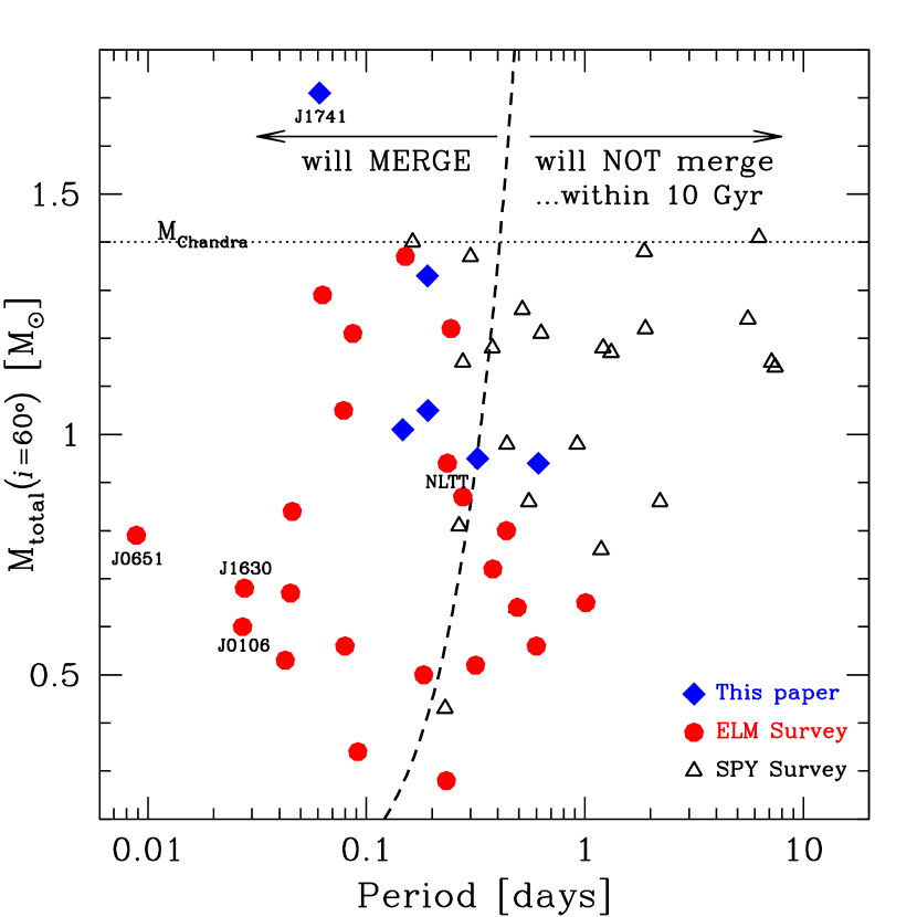
Figure 6.— Binary orbital period versus total system mass for the full ELM Survey and for the Supernova Progenitor Survey (SPY, Koester et al., 2009). We plot total system mass assuming $i=60\arcdeg$ when orbital inclination is unknown, and the correct system mass when inclination is known. WD binaries from SPY are drawn with open triangles, previously published ELM Survey binaries are drawn with solid red circles, and the 6 new ELM WD binaries from this paper are drawn with solid blue diamonds. The dashed line shows the threshold at which a 1:1 mass ratio system will merge in 10 Gyr.

Table 3Merger Systems in the ELM Survey

Object	$T_{\rm eff}$	$\log g$	Mass	$P$	$K$	$M_{2}$	$\tau_{\rm merge}$	$\gamma$	$\mu_{\rm RA}$	$\mu_{\rm Dec}$	Ref
	(K)		$M_{\odot}$	days	km s-1	$M_{\odot}$	Gyr	km s-1	mas yr-1	mas yr-1
J0022$-$1014	18980	7.15	0.33	0.07989	145.6	$\geq 0.19$	$\leq 0.73$	$81$	$-7.8$	$-13.2$	5
J0106$-$1000	16490	6.01	0.17	0.02715	395.2	0.43	0.037	$2$	$20.2$	$-9.6$	6
J0112+1835	9770	5.57	0.16	0.14698	295.3	$\geq 0.62$	$\leq 2.67$	$-121$	$7.8$	$-17.4$	0
J0651+2844	16400	6.79	0.25	0.00885	657.3	0.55	0.0009	$17$	$-3.6$	$-1.2$	2
J0755+4906	13160	5.84	0.17	0.06302	438.0	$\geq 0.81$	$\leq 0.22$	$-51$	$\cdots$	$\cdots$	1
J0818+3536	10620	5.69	0.17	0.18315	170.0	$\geq 0.26$	$\leq 8.89$	$-201$	$\cdots$	$\cdots$	1
J0822+2753	8880	6.44	0.17	0.24400	271.1	$\geq 0.76$	$\leq 8.42$	$-52$	$3.4$	$-19.2$	3
J0849+0445	10290	6.23	0.17	0.07870	366.9	$\geq 0.64$	$\leq 0.47$	$48$	$-0.7$	$-0.4$	3
J0923+3028	18350	6.63	0.23	0.04495	296.0	$\geq 0.34$	$\leq 0.13$	$2$	$-4.2$	$-24.9$	1
J1053+5200	15180	6.55	0.20	0.04256	264.0	$\geq 0.26$	$\leq 0.16$	$12$	$-29.7$	$-31.2$	3,8
J1233+1602	10920	5.12	0.17	0.15090	336.0	$\geq 0.86$	$\leq 2.14$	$-35$	$\cdots$	$\cdots$	1
J1234$-$0228	18000	6.64	0.23	0.09143	94.0	$\geq 0.09$	$\leq 2.69$	$94$	$-14.5$	$-12.3$	5
J1436+5010	16550	6.69	0.24	0.04580	347.4	$\geq 0.46$	$\leq 0.10$	$-30$	$7.8$	$-5.1$	3,8
J1443+1509	14770	6.06	0.17	0.19053	306.7	$\geq 0.83$	$\leq 4.09$	$-172$	$-30.9$	$-53.5$	0
J1630+4233	14670	7.05	0.30	0.02766	295.9	$\geq 0.30$	$\leq 0.03$	$-11$	$2.3$	$-7.3$	7
J1741+6526	9900	5.20	0.16	0.06111	508.0	$\geq 1.09$	$\leq 0.17$	$-70$	$-3.2$	$-4.6$	0
J1840+6423	9100	6.22	0.17	0.19130	272.0	$\geq 0.64$	$\leq 5.00$	$-76$	$-12.4$	$-26.7$	0
J2119$-$0018	10360	5.36	0.17	0.08677	383.0	$\geq 0.75$	$\leq 0.54$	$-28$	$\cdots$	$\cdots$	1
NLTT 11748	8690	6.54	0.18	0.23503	273.4	0.76	7.20	$126$	$236.1$	$-179.2$	4,9,10

References. — (0) this paper; (1) Brown et al. (2010); (2) Brown et al. (2011b); (3) Kilic et al. (2010b); (4) Kilic et al. (2010a); (5) Kilic et al. (2011a); (6) Kilic et al. (2011c); (7) Kilic et al. (2011b); (8) Mullally et al. (2009); (9) Steinfadt et al. (2010); (10) Kawka et al. (2010)

Note. — Measurement errors reported in the references. Proper motions are from USNO-B+SDSS (Munn et al., 2004).

While the merging ELM WD sample is not complete, properties such as orbital period and secondary mass are in principle independent of color and magnitude. Thus we split the merging ELM WD sample into thirds and search for significant correlations among the sample properties.

Looking at Table 4, the six ELM WDs with $<$1.1 hr orbital periods are 6000$\pm$2400 K hotter than the seven ELM WDs with $>$3.5 hr orbital periods. In other words, we observe an absence of cool ELM WDs with short orbital periods. This period-temperature dependence makes sense if the ELM WDs in short orbital period systems merge before they cool. We take this correlation as evidence that common envelope evolution creates ELM WDs directly in short orbital period systems.

The minimum companion masses of the ELM WDs span an order of magnitude, from 0.1 $M_{\odot}$ to 1.1 $M_{\odot}$, and also appear to correlate with ELM WDs’ temperatures. The coolest seven ELM WDs, those with $T_{\rm eff}$$<$10,500 K, have minimum companion masses that are 0.41$\pm$0.23 $M_{\odot}$ larger than the hottest six ELM WDs with $T_{\rm eff}$$>$16,000 K. This result largely comes from our present survey, which targets relatively cool ELM WDs and finds only extreme mass-ratio binaries. Our interpretation is that shorter period binary systems experience increased mass loss during their evolution and end up with lower mass companions. A larger sample is required to establish these trends with increased significance.

Figure 6 compares the distribution of binary orbital period and total system mass for the ELM Survey with that of the Supernova Progenitor Survey (SPY, Napiwotzki et al., 2001; Koester et al., 2009). The SPY survey has measured the velocity variability of $\simeq$1000 WDs, the largest survey of its kind. Our Figure is an adaptation of Geier et al. (2010)’s Figure 4, where we plot total system mass assuming $i=60\arcdeg$ when orbital inclination is unknown, and the correct system mass when inclination is known via ellipsoidal variations and/or eclipses. It is notable that the SPY survey, which samples the full WD population, finds only a handful of systems with orbital periods short enough that they might possibly merge in less than 10 Gyr.

The ELM survey, which targets $\sim$0.2 $M_{\odot}$ WDs, finds almost every object in a system with $\lesssim$1 day orbital period, the majority of which will merge due to gravitational wave radiation in less than 10 Gyr. The merging ELM WD systems are unlikely Type Ia supernovae progenitors, however, because the total mass of the systems is likely below the Chandrasekhar mass. Their most likely evolutionary futures include the formation of stable mass-transfer AM CVn systems and underluminous supernovae, or unstable mass-transfer mergers that form extreme helium stars (RCrB) and single helium-enriched subdwarf O stars (discussed further in Kilic et al., 2010b). One approach to constrain these scenarios is to compare ELM WD merger rates with the formation rates of different classes of objects as attempted in Brown et al. (2011a). A larger, well-defined sample will provide improved constraints, as will follow-up light curves that directly measure the orbital inclination and nature of the unseen binary companions.

We close by noting that at least one-third of the merging ELM WD systems have the kinematics and locations of halo objects. Looking at Table 4, four ELM WD systems (J0112, J0818, J1443, NLTT 11748) have systemic radial velocities $|\gamma|>100$ km s^-1. Proper motions with 5 mas yr^-1 uncertainties are available for 15 of the 19 objects (Munn et al., 2004; Lépine & Shara, 2005). Combining radial velocities and proper motions reveals five systems (J0106, J0818, J1053, J1443, NLTT 11748) with total space velocities $>$200 km s^-1 with respect to the Sun. Thus 6 unique ELM WD systems (32%) have kinematics that indicate a halo origin. In addition to motions, physical locations also support a halo origin. The ELM WDs are not clustered at low Galactic latitudes in our survey, as expected for a disk population, but rather are found equally at high and low Galactic latitudes. The typical ELM WD in our survey has median luminosity $M_{g}=8.5$, apparent magnitude $g_{0}=18.8$, and Galactic latitude $b=43\arcdeg$, and thus is located $\simeq$1 kpc above the Galactic plane. We conclude that ELM WD systems continue to form and merge in both the disk and the halo, a conclusion that has implications for gravitational wave source predictions (Ruiter et al., 2009).

5. CONCLUSION

We present a targeted spectroscopic survey of ELM WDs candidates selected by color. The survey is successful: it is now 71% complete and has uncovered 18 new ELM WDs. Of the 7 ELM WDs with follow-up observations, 6 are compact binary systems and 4 have gravitational wave merger times less than 5 Gyr. The most intriguing new object is J1741+6526, which likely has either a milli-second pulsar binary companion or a massive WD companion making the system a possible supernova Type Ia or .Ia progenitor. Follow-up observations are underway to establish the nature of this system as well as the other ELM WDs.

Based on these initial results, we expect that completing our targeted ELM WD survey will double the number of merging systems in our sample from 19 to $\simeq$40 systems. We expect that photometric follow-up will reveal additional eclipsing systems. Our efficiency for ELM WDs discoveries increases with apparent magnitude such that, if we were to expand our discovery survey to $g\simeq 20.5$, we could in principle double again our sample of ELM WDs (although the observations are more expensive). The absence of short-merger time systems at cooler temperatures suggests that expanding our survey to hotter objects may yield additional $\sim$10 min orbital period ($<$1 Myr merger time) systems. These are directions we will pursue in upcoming observing runs. With a sample of $\sim$100 ELM WDs systems spanning a well-defined range of temperature, we look forward to placing robust constraints on the role of these detached double degenerate binaries as supernovae progenitors and gravitational wave sources.

Appendix A DATA TABLE

Table 4 presents our radial velocity measurements. The Table columns include object name, heliocentric Julian date (based on UTC), heliocentric radial velocity (uncorrected for the WD gravitational redshift), and velocity error.      [See on-line journal or tab4.dat in the arXiv submission.]

References

- Abazajian et al. (2009) Abazajian, K. N., Adelman-McCarthy, J. K., Agüeros, M. A., et al. 2009, ApJS, 182, 543
- Allende Prieto et al. (2006) Allende Prieto, C., Beers, T. C., Wilhelm, R., et al. 2006, ApJ, 636, 804
- Bergeron et al. (1995) Bergeron, P., Wesemael, F., & Beauchamp, A. 1995, PASP, 107, 1047
- Bildsten et al. (2007) Bildsten, L., Shen, K. J., Weinberg, N. N., & Nelemans, G. 2007, ApJ, 662, L95
- Brown et al. (2009) Brown, W. R., Geller, M. J., & Kenyon, S. J. 2009, ApJ, 690, 1639
- Brown et al. (2005) Brown, W. R., Geller, M. J., Kenyon, S. J., & Kurtz, M. J. 2005, ApJ, 622, L33
- Brown et al. (2006) —. 2006, ApJ, 640, L35
- Brown et al. (2010) Brown, W. R., Kilic, M., Allende Prieto, C., & Kenyon, S. J. 2010, ApJ, 723, 1072
- Brown et al. (2011a) —. 2011a, MNRAS, 411, L31
- Brown et al. (2011b) Brown, W. R., Kilic, M., Hermes, J. J., Allende Prieto, C., Kenyon, S. J., & Winget, D. E. 2011b, ApJ, 737, L23
- Eisenstein et al. (2006) Eisenstein, D. J. et al. 2006, ApJS, 167, 40
- Fabricant et al. (1998) Fabricant, D., Cheimets, P., Caldwell, N., & Geary, J. 1998, PASP, 110, 79
- Fuller & Lai (2011) Fuller, J. & Lai, D. 2011, ApJ, submitted (arXiv:1108.4910)
- Geier et al. (2010) Geier, S., Heber, U., Kupfer, T., & Napiwotzki, R. 2010, A&A, 515, A37
- Holberg & Bergeron (2006) Holberg, J. B. & Bergeron, P. 2006, AJ, 132, 1221
- Kawka et al. (2010) Kawka, A., Vennes, S., & Vaccaro, T. R. 2010, A&A, 516, L7
- Kenyon & Garcia (1986) Kenyon, S. J. & Garcia, M. R. 1986, AJ, 91, 125
- Kilic et al. (2010a) Kilic, M., Allende Prieto, C., Brown, W. R., Agüeros, M. A., Kenyon, S. J., & Camilo, F. 2010a, ApJ, 721, L158
- Kilic et al. (2011a) Kilic, M., Brown, W. R., Allende Prieto, C., Agüeros, M. A., Heinke, C., & Kenyon, S. J. 2011a, ApJ, 727, 3
- Kilic et al. (2010b) Kilic, M., Brown, W. R., Allende Prieto, C., Kenyon, S. J., & Panei, J. A. 2010b, ApJ, 716, 122
- Kilic et al. (2009) Kilic, M., Brown, W. R., Allende Prieto, C., Swift, B., Kenyon, S. J., Liebert, J., & Agüeros, M. A. 2009, ApJ, 695, L92
- Kilic et al. (2011b) Kilic, M., Brown, W. R., Hermes, J. J., Allende Prieto, C., Kenyon, S. J., Winget, D. E., & Winget, K. I. 2011b, MNRAS, 418, L157
- Kilic et al. (2011c) Kilic, M., Brown, W. R., Kenyon, S. J., Allende Prieto, C., Andrews, J., Kleinman, S. J., Winget, K. I., Winget, D. E., & Hermes, J. J. 2011c, MNRAS, 413, L101
- Koester (2008) Koester, D. 2008, ArXiv:0812.0482
- Koester et al. (2009) Koester, D., Voss, B., Napiwotzki, R., Christlieb, N., Homeier, D., Lisker, T., Reimers, D., & Heber, U. 2009, A&A, 505, 441
- Kurtz & Mink (1998) Kurtz, M. J. & Mink, D. J. 1998, PASP, 110, 934
- Landau & Lifshitz (1958) Landau, L. D. & Lifshitz, E. M. 1958, The classical theory of fields (Oxford: Pergamon Press)
- Lépine & Shara (2005) Lépine, S. & Shara, M. M. 2005, AJ, 129, 1483
- Marsh et al. (1995) Marsh, T. R., Dhillon, V. S., & Duck, S. R. 1995, MNRAS, 275, 828
- Marsh et al. (2004) Marsh, T. R., Nelemans, G., & Steeghs, D. 2004, MNRAS, 350, 113
- Massey et al. (1988) Massey, P., Strobel, K., Barnes, J. V., & Anderson, E. 1988, ApJ, 328, 315
- Mullally et al. (2009) Mullally, F., Badenes, C., Thompson, S. E., & Lupton, R. 2009, ApJ, 707, L51
- Munn et al. (2004) Munn, J. A. et al. 2004, AJ, 127, 3034
- Napiwotzki et al. (2001) Napiwotzki, R., Christlieb, N., Drechsel, H., et al. 2001, Astronomische Nachrichten, 322, 411
- Nebot Gómez-Morán et al. (2011) Nebot Gómez-Morán, A., Gänsicke, B. T., Schreiber, M. R., et al. 2011, A&A, accepted
- Nelemans et al. (2005) Nelemans, G., Napiwotzki, R., Karl, C., et al. 2005, A&A, 440, 1087
- Panei et al. (2007) Panei, J. A., Althaus, L. G., Chen, X., & Han, Z. 2007, MNRAS, 382, 779
- Parsons et al. (2011) Parsons, S. G., Marsh, T. R., Gänsicke, B. T., Drake, A. J., & Koester, D. 2011, ApJ, 735, L30
- Piro (2011) Piro, A. L. 2011, ApJ, 740, L53
- Pyrzas et al. (2011) Pyrzas, S., Gaensicke, B. T., Brady, S., et al. 2011, MNRAS, accepted
- Roelofs et al. (2007) Roelofs, G. H. A., Groot, P. J., Benedict, G. F., McArthur, B. E., Steeghs, D., Morales-Rueda, L., Marsh, T. R., & Nelemans, G. 2007, ApJ, 666, 1174
- Ruiter et al. (2009) Ruiter, A. J., Belczynski, K., Benacquista, M., & Holley-Bockelmann, K. 2009, ApJ, 693, 383
- Schmidt et al. (1989) Schmidt, G. D., Weymann, R. J., & Foltz, C. B. 1989, PASP, 101, 713
- Serenelli et al. (2001) Serenelli, A. M., Althaus, L. G., Rohrmann, R. D., & Benvenuto, O. G. 2001, MNRAS, 325, 607
- Steinfadt et al. (2010) Steinfadt, J. D. R., Kaplan, D. L., Shporer, A., Bildsten, L., & Howell, S. B. 2010, ApJ, 716, L146
- Vennes et al. (2011) Vennes, S., Thorstensen, J. R., Kawka, A., et al. 2011, ApJ, 737, L16
- Zorotovic et al. (2011) Zorotovic, M., Schreiber, M. R., & Gänsicke, B. T. 2011, A&A, accepted