HU-EP-11/54

Hexagon remainder function in the limit
of self-crossing up to three loops

Harald Dorn, Sebastian Wuttke

Institut für Physik der Humboldt-Universität zu Berlin,
Newtonstraße 15, D-12489 Berlin, Germany

Abstract

We consider Wilson loops in planar ${\cal N}=4$ SYM for null polygons in the limit of two crossing edges. The analysis is based on a renormalisation group technique. We show that the previously obtained result for the leading and next-leading divergent term of the two loop hexagon remainder is in full agreement with the appropriate continuation of the exact analytic formula for this quantity. Furthermore, we discuss the coefficients of the leading and next-leading singularity for the three loop remainder function for null $n$-gons with $n\geq 6$.

1 Introduction

Recently, Wilson loops for polygonal null contours in planar ${\cal N}=4$ supersymmetric Yang-Mills theory have attracted a lot of attention. This interest is mainly due to their correspondence to gluon scattering amplitudes. It has been first established at strong coupling by string theoretical arguments [1] and later verified also at weak coupling [2]. On the perturbative side one expresses the logarithm of the Wilson loop as the sum of the well-known BDS structure [3] plus some remainder function. Then the determination of this remainder function in higher and higher loop order comes into the main focus.

At two-loop order the complete hexagon remainder [4, 5] and the octagon remainder for restricted configurations [6] are available. Furthermore, the differential of the remainder has been analysed for arbitrary null $n$-gons yielding explicit analytic formulæ  for some parts while only giving the symbol for other terms [7]. At three-loop level a recent paper has bootstrapped the symbol of the hexagon remainder [8]. The results of [7, 8] have been obtained by combining symmetry arguments and constraints provided by operator product expansions and by collinear as well as by multi Regge limits.

Further independent information on the remainder functions can be extracted out of the study of the limit of self-crossing contours. Such an analysis can be based on standard renormalisation (RG) group techniques. It has been started for the two-loop hexagon remainder in [9] and continued in our previous paper on the two-loop octagon case [10]. To be more precise, the difference between the two papers is not so much an issue of hexagon versus octagon. A self-crossing polygon can be one with crossing edges or one with two coinciding vertices. For a hexagon, due to the null condition, only the first case can be realized, for octagons and higher $n$-gons both cases are possible. In the limit with crossing edges the cross-ratio $u$ formed out of the four endpoints of the edges approaches the number one, and the remainder develops singularities in powers of $\log(u-1)$ with pure numerical coefficients. In the second type of limit one gets divergences in powers of the logarithm of a product of four cross-ratios. This time the coefficients depend on the cross-ratio formed out of the four vertices adjacent to the two coinciding ones.

The aim of this paper is twofold. First we want to fill a gap left by [9, 10]. As described in detail in these papers, the goal to control the short distances singularities of the remainder function in the approach to a self-crossing configuration is achieved in the following way. Using dimensional regularisation, one analyses the additional UV-singularities due to the crossing directly in a self-crossing configuration. Then one interprets the near to self-crossing situations as some alternative regularisation, providing a translation of powers in $1/\epsilon$ into powers of the negative logarithm of some distance. Due to the usual scheme ambiguities, in this translation rule numerical factors remain open. We want to fix these numbers with arguments based on our approach before we show the agreement of the two-loop hexagon result of [9, 10] with the appropriate analytic continuation of the complete remainder function of [5].

The second task concerns the calculation of the leading plus next-leading divergent terms for the three-loop hexagon (or even $n$-gon) remainder function for the limit of two edges approaching the self-crossing configuration.

2 RG technique for the remainder function at two and three loop level

Self-crossing Wilson loops were first studied for QCD and it was shown [11, 12, 13, 14] that they can be multiplicatively renormalised using a $\mathcal{Z}$ matrix

$$\mathcal{W}_{a}~{}=~{}\mathcal{Z}_{ab}~{}\mathcal{W}_{b}^{\text{ren}}~{}.$$ (1)

$\{\mathcal{W}_{a}\}$ is the set of mixing Wilson loop operators, $a\in\{1,2\}$.
With $\mathcal{U}(\mathcal{C}):=\frac{1}{N}~{}\text{tr}~{}\mathcal{P}~{}\exp\left(ig\int_{\mathcal{C}}A^{\mu}\text{d}x_{\mu}\right)$ for $\text{SU}(N)$ theory. $\mathcal{W}_{1}$ and $\mathcal{W}_{2}$ are defined by

$$\mathcal{W}_{1}:=\langle\mathcal{U}(\mathcal{C})\rangle~{},~{}~{}\mathcal{W}_{2}:=\langle\mathcal{U}(\mathcal{C}^{\text{upper}})\mathcal{U}(\mathcal{C}^{\text{lower}})\rangle~{}.$$ (2)

In our case all contours $\mathcal{C}^{\text{upper}}$, $\mathcal{C}^{\text{lower}}$ and $\mathcal{C}$ are light-like closed polygons. $\mathcal{C}$ is the full $n$-cusps self-crossing contour (see fig.1) and $\mathcal{C}^{\text{upper}}$ and $\mathcal{C}^{\text{lower}}$ are the two sub-contours starting and ending at the crossing point.

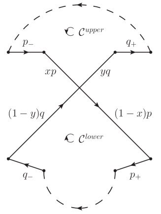
Figure 1: A self-crossing Wilson loop with crossing edges $p$ and $q$. The dashed lines represent any light-like continuation. The dimensionless parameters $x,y\in(0,1)$ define where the crossing is located exactly.

The vertices of the polygons are denoted by $x_{i}$, and because of the correspondence to scattering amplitudes we call $p_{i}=(x_{i+1}-x_{i})$ a momentum. The two crossing edges (momenta) are denoted by $p$ and $q$, and the fractions that determine the crossing point by $x$ and $y$ (see fig.1). In the ’t Hooft limit under consideration, $\mathcal{W}_{2}$ factorises

$$\mathcal{W}_{2}=\langle\mathcal{U}(\mathcal{C}^{\text{upper}})\rangle\langle\mathcal{U}(\mathcal{C}^{\text{lower}})\rangle~{},$$ (3)

and the $\mathcal{Z}$ -matrix has the triangular form

$$\mathcal{Z}=\begin{pmatrix}\mathcal{Z}_{11}&\mathcal{Z}_{12}\\ 0&\mathcal{Z}_{22}\end{pmatrix}~{}.$$ (4)

Then also the anomalous dimension matrix

$$\Gamma:=\mathcal{Z}^{-1}\mu\frac{d}{d\mu}\mathcal{Z}~{}\Big{|}_{g_{\text{bare}}{\text{~{}fixed}}}~{},$$ (5)

is upper triangular.

Originally, the renormalisation of Wilson loops has been studied for contours without light-like pieces. Then the $\mathcal{Z}$-factors as well as the anomalous dimensions depend on the coupling constant and the angles at the cusps and at the self-crossing. In the light-like limit the angles become divergent and make the related original RG equation ill-defined. Following [16] one nevertheless can get a modified RG equation which has the same structure as the original one, but with RG scale dependent anomalous dimensions. For more details and references we refer to [16],[14],[9, 10].

The RG equation to start with is then $\mu\frac{\partial}{\partial\mu}~{}\mathcal{W}_{a}^{\text{ren}}~{}=~{}-~{}\Gamma_{ab}~{}\mathcal{W}_{b}^{\text{ren}}~{},~{}a,b\in\{1,2\}~{}.$ It implies for $\mathcal{W}_{1}^{\text{ren}}$

$$\mu\frac{\partial}{\partial\mu}~{}\log\mathcal{W}_{1}^{\text{ren}}~{}=~{}-~{}\Gamma_{12}~{}\frac{\mathcal{W}_{2}^{\text{ren}}}{\mathcal{W}_{1}^{\text{ren}}}~{}-~{}\Gamma_{11}~{}.$$ (6)

For the following analysis we need formulæ  expressing $\log\mathcal{W}_{a}^{\text{ren}}$ in terms of its unrenormalised partners and the entries of the anomalous dimension matrix. Preparing this for the use up to three loop level requires a bit more effort as in [9, 10]. A further comment concerns the fact, that for self-crossing polygons with crossing edges, the $\mathcal{Z}$-factors no longer factorise into a cusp and a crossing part. Therefore, one has to look for the relation of the overall $\mathcal{Z}$-matrix in (1) and the total $\Gamma$-matrix in (6).

The anomalous dimension of a Wilson loop for a self-crossing null polygon is given [16],[14],[9] via

$$\Gamma=~{}\begin{pmatrix}1&0\\ 0&1\end{pmatrix}~{}\frac{\Gamma_{\text{cusp}}(a)}{2}\sum_{k\in\text{cusps}}\log\left(-s_{k}\mu^{2}\right)+~{}\begin{pmatrix}A&\gamma_{12}(a)\\ 0&B\end{pmatrix}~{},$$ (7)

where

$$A= \frac{\Gamma_{\text{cusp}}(a)}{2}\left(\log(-2pp_{-}\mu^{2})+\log(-2pp_{+}\mu^{2})+\log(-2qq_{-}\mu^{2})+\log(-2qq_{+}\mu^{2})\right)~{},$$

$$B= \frac{\Gamma_{\text{cusp}}(a)}{2}\left(\log(-2pp_{-}x\mu^{2})+\log(-2pp_{+}(1-x)\mu^{2})+\log(-2qq_{-}(1-y)\mu^{2})\right.$$

$$\left.+\log(-2qq_{+}y\mu^{2})\right)+\gamma_{22}(a)\left(\log(-sxy\mu^{2})+\log(-s(1-x)(1-y)\mu^{2})\right)~{},$$

with $a=\frac{g^{2}N}{8\pi^{2}}$ and $s=2pq$. By $\sum_{k\in\text{cusps}}$ we denote all cusps that are not adjacent to the crossing and by $s_{k}=(x_{k-1}-x_{k+1})^{2}$ the Mandelstam variables at the cusps.

All entries in the anomalous dimension matrix that are proportional to $\Gamma_{\text{cusp}}$ originate from UV divergences that are related to cusps. The cusps adjacent to the crossing contribute in a different manner to $\mathcal{W}_{1}$ and $\mathcal{W}_{2}$. For $\mathcal{W}_{1}$ the full momenta $p$ and $q$ are relevant and for $\mathcal{W}_{2}$ only fractions thereof. Therefore, also the cusp terms in the anomalous dimension matrix are not a multiple of the unit matrix. In the anomalous dimension matrix $\gamma_{12}$ and $\gamma_{22}$ are functions of the coupling only. The one-loop results in planar limit are

$$\gamma_{12}^{(1)}~{}=~{}\pm~{}\text{sgn}(pq)~{}2\pi i~{}~{},~{}~{}~{}~{}\gamma_{22}^{(1)}~{}=~{}1~{}~{},~{}~{}~{}~{}\Gamma^{(1)}_{\text{cusp}}~{}=~{}2~{}.$$ (8)

We will later comment on $\gamma_{12}^{(1)}$ as this entry plays an important role for the analytic continuations discussed in the next section.

Now we consider (5) as a differential equation in $\mu$ for $\mathcal{Z}$. Because of the upper triangular structure of $\mathcal{Z}$ and $\Gamma$ we find

$$\mu\frac{d}{d\mu}\log\mathcal{Z}_{11}~{} =\Gamma_{11}~{},~{}~{}~{}~{}~{}~{}~{}~{}\mu\frac{d}{d\mu}\mathcal{Z}_{12}=\mathcal{Z}_{11}\Gamma_{12}+\mathcal{Z}_{12}\Gamma_{22}~{},$$ (9)

$$\mu\frac{d}{d\mu}\log\mathcal{Z}_{22}~{} =\Gamma_{22}~{}.$$

We solve this as an expansion in powers of $a$, i.e. $\Gamma=\sum_{l}a^{l}\Gamma^{(l)}$ and similar for $\mathcal{Z}$. Keeping in mind that the $\mu$ derivative has to be taken at fixed bare coupling and that $a=a_{\text{bare}}\mu^{-2\epsilon}$, the first two equations give for a $n$-gon

$$\mathcal{Z}_{11}^{(0)} =1~{},~{}~{}~{}~{}~{}\mathcal{Z}_{11}^{(1)}~{}=-\frac{n\Gamma^{(1)}_{\text{cusp}}}{4\epsilon^{2}}-\frac{\Gamma_{11}^{(1)}}{2\epsilon}~{},$$

$$\mathcal{Z}_{22}^{(0)} =1~{},~{}~{}~{}~{}~{}\mathcal{Z}_{22}^{(1)}~{}=-\frac{n\Gamma^{(1)}_{\text{cusp}}+4\gamma_{22}^{(1)}}{4\epsilon^{2}}-\frac{\Gamma_{22}^{(1)}}{2\epsilon}~{}.$$ (10)

Now we solve (9) for $\mathcal{Z}_{12}$. A priori it is clear that $\mathcal{Z}_{12}^{(0)}=0$. At order $\mathcal{O}(a)$ we find

$$\Gamma^{(1)}_{12}a=\mu\frac{d}{d\mu}\left(\mathcal{Z}_{12}^{(1)}a\right)~{}~{}\Longrightarrow~{}~{}\mathcal{Z}_{12}^{(1)}=-\frac{\gamma_{12}^{(1)}}{2\epsilon}~{}.$$ (11)

At order $\mathcal{O}(a^{2})$ eq.(9) means

$$a^{2}\left(\Gamma_{12}^{(2)}+\mathcal{Z}_{11}^{(1)}\Gamma_{12}^{(1)}+\mathcal{Z}_{12}^{(1)}\Gamma_{22}^{(1)}\right)=\mu\frac{d}{d\mu}\left(\mathcal{Z}_{12}^{(2)}a^{2}\right)~{}.$$ (12)

Integration yields

$$\mathcal{Z}_{12}^{(2)}=\frac{(n\Gamma^{(1)}_{\text{cusp}}+\gamma_{22}^{(1)})\gamma_{12}^{(1)}}{8\epsilon^{3}}+\frac{\gamma_{12}^{(1)}\left(\Gamma_{11}^{(1)}+\Gamma_{22}^{(1)}\right)}{8\epsilon^{2}}-\frac{\gamma_{12}^{(2)}}{4\epsilon}~{}.$$ (13)

Expanding the logarithms of the Wilson loops in powers of $a$ one gets from (1) within minimal subtracted dimensional regularisation

$$\log\mathcal{W}_{1}^{\text{ren}(1)} =\text{MS}\Big{[}\log\mathcal{W}_{1}^{(1)}\Big{]}=\mathcal{W}_{1}^{\text{ren}(1)}~{},$$

$$\log\mathcal{W}_{1}^{\text{ren}(2)} =\text{MS}\Big{[}\log\mathcal{W}_{1}^{(2)}+\mathcal{Z}_{12}^{(1)}\left(\mathcal{W}_{1}^{\text{ren}(1)}-\mathcal{W}_{2}^{\text{ren}(1)}\right)\Big{]}~{},$$ (14)

$$\log\mathcal{W}_{1}^{\text{ren}(3)} =\text{MS}\Big{[}\log\mathcal{W}_{1}^{(3)}~{}-~{}T_{1}~{}-~{}T_{2}\Big{]}~{},$$

with $\text{MS}\big{[}~{}.~{}\big{]}$ denoting minimal subtraction and

$$T_{1} :=\mathcal{Z}_{12}^{(1)}\left(\frac{1}{2}\left(\mathcal{W}_{1}^{\text{ren}(1)}-\mathcal{W}_{2}^{\text{ren}(1)}\right)^{2}-\log\mathcal{W}_{1}^{\text{ren}(2)}+\log\mathcal{W}_{2}^{\text{ren}(2)}\right)~{},$$ (15)

$$T_{2} :=\left(\left(\mathcal{Z}_{12}^{(1)}\right)^{2}+\mathcal{Z}_{12}^{(1)}\mathcal{Z}_{11}^{(1)}-\mathcal{Z}_{12}^{(2)}\right)\left(\mathcal{W}_{1}^{\text{ren}(1)}-\mathcal{W}_{2}^{\text{ren}(1)}\right)~{}.$$ (16)

In contrast, due to the triangular form of the $\mathcal{Z}$-matrix in (4), for $\mathcal{W}_{2}$ one simply has

$$\log\mathcal{W}_{2}^{\text{ren}(l)}~{}=~{}\text{MS}\Big{[}~{}\log\mathcal{W}_{2}^{(l)}~{}\Big{]}~{}.$$ (17)

For the logarithms of the Wilson loops we insert the BDS Ansatz [3], corrected by the remainder function $\mathcal{R}$ .

$$\log\mathcal{W}=\sum_{l=1}^{\infty}a^{l}\left(f^{(l)}(\epsilon)w(l~{}\epsilon)+C^{(l)}\right)+\mathcal{R}+\mathcal{O}(\epsilon)~{},$$ (18)

where $C^{(l)}$ are (known) numbers, $f^{(l)}(\epsilon)=f_{0}^{(l)}+\epsilon~{}f_{1}^{(l)}+\epsilon^{2}~{}f_{2}^{(l)}$, and $w(\epsilon)$ is the one loop contribution

$$w(\epsilon)~{}=~{}-\frac{1}{2\epsilon^{2}}\sum_{k=1}^{n}\left(-\mu^{2}s_{k}\pm i\varepsilon\right)^{\epsilon}+F(\mu^{2},\epsilon,\{s\})~{}.$$ (19)

Here $n$ is again the number of cusps and $s_{k}$ the Mandelstam variable associated with the $k$’th cusp. $F(\mu^{2},\epsilon,\{s\})$ is the so-called one-loop finite contribution. It remains finite for $\epsilon\rightarrow 0$ in a generic $n$-gon configuration, but develops poles in a self-crossing case. The $a$-expansion of $\mathcal{R}$ starts at $\mathcal{O}(a^{2})$.

It will be convenient to include the $\mathcal{O}(\epsilon)$ term in (18) into $\mathcal{R}$ i.e. to use

$$\mathcal{R}(\mu^{2},\epsilon,\{s\})=\log\mathcal{W}-\Big{[}\text{BDS}\Big{]}~{},$$ (20)

where $\{s\}$ is the set of all Mandelstam variables. For a generic Wilson loop

$$\mathcal{R}(\{u\})=\lim_{\epsilon\rightarrow 0}~{}\mathcal{R}(\mu^{2},\epsilon,\{s\})$$ (21)

is finite, independent of $\mu^{2}$ and only a function of conformal invariants $\{u\}$. However, if the Wilson loop contains a self-crossing the new divergences at the crossing point will lead to poles in $\epsilon$ in $\mathcal{R}(\mu^{2},\epsilon,\{s\})$.

Our aim is to calculate the (most) divergent terms. Plugging the BDS Ansatz including the remainder function into the renormalisation group equation (6) one can calculate $\text{MS}\Big{[}\mathcal{R}(\mu^{2},\epsilon,\{s\})\Big{]}$ using (14),(20). From this expression one can deduce the most divergent terms, as we will do explicitly for the three-loop remainder in section 4. Then, considering a slight off self-crossing configuration as an alternative regularisation, one can relate those divergent terms to divergences of $\mathcal{R}(\{u\})$ when the cross-ratios approach their self-crossing values. This method works for the leading and next-leading divergences at all orders in $a$. To calculate those terms, only one-loop information on the anomalous dimension matrix is needed. The leading and next-leading contributions for $\mathcal{R}^{(2)}$ were calculated in [9]. When this paper was written, the compact analytic result of [5] was not yet available. The remainder function presented in [5] is finite for these values of the cross ratios. However, the remainder function is multi-valued. Wilson loops for null hexagons with all Mandelstam variables in the Euclidean region can never be conformal to self-intersecting ones. The divergent terms are created by the analytic continuation to a self-crossing region, as we will explain in the next section.

3 Analytic continuation from the Euclidean region

Figure 2: The self-crossing hexagon and its mixing partner.

For the comparison of the asymptotic result of [9] with certain analytic continuations of the exact hexagon remainder of [5] one has to be very careful with the $i\varepsilon$-prescription and the induced signs of imaginary parts.

With respect to the correspondence between Wilson loops and scattering amplitudes it has been argued, that for the use in this duality one has to switch the sign of the $i\varepsilon$-prescription in the gluon propagator relative to that in the standard position space propagator [9],[17]. This switch leads to a change of the sign of the one loop entry $\gamma_{12}^{(1)}$ of the crossing anomalous dimension matrix [9] in comparison to the original calculation of [14].

Denoting by $p$ and $q$ the vectors spanning the crossing edges of the hexagon as in fig.2 one gets according to [14]

$$pq<0 : \gamma_{12}^{(1)}=-2\pi i\coth\beta~{},~{}~{}~{}~{}\cosh\beta=-\frac{pq}{\sqrt{p^{2}q^{2}}}$$

$$pq>0 : \gamma_{12}^{(1)}=2\pi i\coth\gamma~{},~{}~{}~{}~{}\cosh\gamma=\frac{pq}{\sqrt{p^{2}q^{2}}}~{}.$$ (22)

Keeping now in addition the option of both signs in the $i\varepsilon$-prescription, we get in the light-like limits ($\beta\rightarrow\infty$, $\gamma\rightarrow\infty$)

$$\gamma^{(1)}_{12}~{}=~{}\pm~{}\mbox{sgn}(pq)~{}2\pi i~{}.$$ (23)

Here the upper alternative stands for the standard choice and the lower one for Georgiou’s switched version. Let us also introduce the following abbreviation

$$\mathcal{X}:=x~{}y~{}(1-x)~{}(1-y)~{}~{},~{}~{}~{}~{}x,y\in(0,1)~{}.$$ (24)

After this preparation we get the remainder function in a self-crossing configuration for $pq<0$ as

$$\mathcal{R}^{(2)}=\mp~{}\frac{\pi i}{4}\left(\epsilon^{-3}+2\log\left(|2pq|\mu^{2}\mathcal{X}\right)~{}\epsilon^{-2}\right)+\frac{\pi^{2}}{2}~{}\epsilon^{-2}+{\cal O}(\epsilon^{-1})~{},$$ (25)

and for $pq>0$ as

$$\mathcal{R}^{(2)}=\pm~{}\frac{\pi i}{4}\left(\epsilon^{-3}+2\log\left(2pq\mu^{2}\mathcal{X})\right)~{}\epsilon^{-2}\right)~{}~{}+~{}~{}{\cal O}(\epsilon^{-1})~{}.$$ (26)

The light-like closed hexagon has three conformal invariants $u_{1}$, $u_{2}$ and $u_{3}$, where

$$u_{1}:=\frac{x_{13}^{2}~{}x_{46}^{2}}{x_{14}^{2}~{}x_{36}^{2}}~{},~{}~{}u_{2}:=\frac{x_{15}^{2}~{}x_{24}^{2}}{x_{14}^{2}~{}x_{25}^{2}}~{},~{}~{}u_{3}:=\frac{x_{35}^{2}~{}x_{26}^{2}}{x_{25}^{2}~{}x_{36}^{2}}~{},$$ (27)

and $x_{ij}^{2}=(x_{i}-x_{j})^{2}$. For self-crossing hexagons the kinematics are restricted such that one cross ratio equals one and the remaining two cross ratios are equal to each other. We follow the choice of [9] and use $u_{2}=1$.

We now want to translate the information (25),(26) into a statement on the remainder function in the limit where one approaches a self-crossing situation with $u_{2}=1$, coming from a generic configuration without self-crossing. Denoting by $z$ the vector between the points marked by the fractions $x$ and $y$ on the edges $p$ and $q$, respectively, one gets (see fig.2)

$$u_{2}-1~{}=~{}\frac{2pq~{}z^{2}-4(qz)(pz)}{(-2y(1-x)pq+{\cal O}(z))(-2x(1-y)pq+{\cal O}(z))}~{}.$$ (28)

Writing the arbitrary vector $z$ as $z=\alpha p+\beta q+z_{\perp}$ with $pz_{\perp}=qz_{\perp}=0,~{}z_{\perp}^{2}\leq 0$, the nominator of (28) turns out to be equal to $2pq~{}z_{\perp}^{2}$. This implies that for $pq<0$
( $pq>0$ ) the approach to a self-crossing situation is possible only with $u_{2}\rightarrow 1$ from above ( below ). For $pq<0$ we get from (28)

$$\log\Big{(}\frac{1}{-z_{\perp}^{2}\mu^{2}}\Big{)}~{}=~{}-\log(u_{2}-1)~{}-~{}\log\big{(}-2pq\mu^{2}\mathcal{X}\big{)}~{}+~{}{\cal O}(z^{2})~{}.$$ (29)

For $pq>0$ it is more convenient to use instead

$$\log\Big{(}\frac{1}{-z_{\perp}^{2}\mu^{2}}\Big{)}~{}=~{}-\log(1-u_{2})~{}-~{}\log\big{(}2pq\mu^{2}\mathcal{X}\big{)}~{}+~{}{\cal O}(z^{2})~{}.$$ (30)

Then all terms in (29) and (30) are real. While in the limit under consideration in both equations the l.h.s and the first term of the r.h.s. diverge, the second r.h.s. term stays finite.

Considering dimensional regularisation and point splitting via the introduction of the separation vector $z$ as two regularisations of the UV divergences due to the self-crossing, one expects a translation rule of the type

$$\frac{1}{\epsilon^{m}}~{}\Leftrightarrow~{}\alpha_{m}~{}\log^{m}\Big{(}\frac{1}{-z_{\perp}^{2}\mu^{2}}\Big{)}~{}.$$ (31)

In appendix B we derive, with some heuristic arguments, a general translation rule for arbitrary loop order. For the two-loop case it implies $\alpha_{3}=2/3$ and $\alpha_{2}=1$. This yields for $pq<0$

$$\mathcal{R}^{(2)}~{}=~{}\pm~{}\frac{i\pi}{6}\log^{3}(u_{2}-1)~{}+~{}\frac{\pi^{2}}{2}\log^{2}(u_{2}-1)~{}+~{}{\cal O}\big{(}\log(u_{2}-1)\big{)}~{},$$ (32)

and for $pq>0$

$$\mathcal{R}^{(2)}~{}=~{}\mp~{}\frac{i\pi}{6}\log^{3}(1-u_{2})~{}~{}+~{}~{}{\cal O}\big{(}\log(1-u_{2})\big{)}~{}.$$ (33)

At this stage we want to stress an observation, which gives additional support to our translation rule from appendix B. The relative weight $\alpha_{3}/\alpha_{2}$ is just the right one to prevent the appearance of the not conformally invariant part of the coefficient of $1/\epsilon^{2}$ in (25),(26) in the final result for $\mathcal{R}^{(2)}~{}$!

The complete analytic result of [5] has the form

$$\mathcal{R}^{(2)}~{}=~{}-\frac{1}{2}\mbox{Li}_{4}(1-1/u_{2})~{}-~{}\frac{1}{8}\big{(}\mbox{Li}_{2}(1-1/u_{2})\big{)}^{2}~{}+~{}\dots~{}.$$ (34)

It has been derived in the Euclidean region where all distances between non adjacent vertices of the hexagon are space-like. The dots in (34) stand for terms which for sure are not a source for a divergent contribution in our self-crossing limit. Staying in the first sheet of the Riemann surface of the polylogarithms, which is defined by the Euclidean region, one hits no singularity at $u_{2}=1$, i.e. $v:=1-1/u_{2}=0$. However, there is a singularity at $v=0$ in the second sheet, which can be reached via encircling the branch point at $v=1$, which is the starting point for a cut extending along the real axis from $1$ to $+\infty$. It is due to the continuation of the discontinuity across the cut

$$\mbox{Li}_{n}(v+i\varepsilon)-\mbox{Li}_{n}(v-i\varepsilon)=\frac{2\pi i\log^{n-1}v}{(n-1)!}~{}.$$ (35)

What concerns real hexagon configurations, for $pq<0$ one approaches $v=0$ from above and the logarithms stay real. For $pq>0$ the approach proceeds from negative values of $v$ and the sign of the imaginary part matters.

A starting point in the Euclidean region necessarily has $u_{2}>0$ i.e. $v<1$. Encircling $v=1$ in a counterclockwise (clockwise) manner and approaching then $v=0$ from above gives just the standard (switched) alternative in (32).

Encircling $v=1$ in a clockwise (counterclockwise) manner, going then to negative values of $v$ via a detour around $v=0$ with the same orientation and the approach to $v=0$ from below gives the standard (switched) alternative in (33).

To finish the proof that the complete analytic result of [5] implies our formulæ  for the approach to a self-crossing configuration, one still has to clarify a subtlety. There is no one to one correspondence between the points in the space of cross-ratios and the classes of conformally equivalent hexagon configurations. Therefore, the above identification of suitable paths for analytic continuation in the cross-ratios still does not necessarily mean that these paths can be generated by smooth deformations of the hexagon from the Euclidean region. To fill this gap, we construct in appendix A an explicit example for a smooth deformation of a configuration in the Euclidean region to a self-crossing configuration with $pq<0$. In this case $1/u_{2}$ goes from one to zero and back to one. Combining the “reflection” at $1/u_{2}=0$ with an encircling, we just get the paths in $z=1-1/u_{2}$ described above in connection with (32). Even more, the orientation turns out to be correct if the encircling is generated by introducing an $i\varepsilon$-prescription in the cross-ratios by replacing the factors $(x_{j}-x_{k})^{2}$ by $(x_{j}-x_{k})^{2}\mp i\varepsilon$ just in the same manner as in the gluon propagator.

4 Three-loop remainder function

We are interested in the leading and next-leading divergences of the remainder function of a $n$-sided light-like closed Wilson loop (for $n\geq 6$) in $\mathcal{N}=4$ SYM in the limit of two crossing edges. Expanding the integrated version of (6) in powers of $a$ one gets with (14),(15),(16),(20)

$$\text{MS}\Big{[}[\text{BDS}]^{(3)}+\mathcal{R}^{(3)}(\mu,\epsilon,p_{i})-T_{1}-T_{2}\Big{]}=\int\Big{(}-T_{3}-\Gamma_{11}^{(3)}\Big{)}~{}\frac{\text{d}\mu}{\mu}~{},$$ (36)

where

$$T_{3}:=\left(\Gamma_{12}~{}\frac{\mathcal{W}_{2}^{\text{ren}}}{\mathcal{W}_{1}^{\text{ren}}}\right)^{(3)}~{}.$$ (37)

For extracting the leading and next-leading divergences of $\mathcal{R}^{(3)}$, we have to keep track of the leading and next-leading terms in $\log\mu^{2}$. Anticipating the leading terms to be $\mathcal{O}(\log^{5}\mu^{2})$, we will discard all terms of $\mathcal{O}(\log^{3}\mu^{2})$ and lower. For example the $[\text{BDS}]^{(3)}$- terms are only $\mathcal{O}(\log^{2}\mu^{2})$. Similarly $\int\Gamma_{11}\text{d}\log\mu$ is also $\mathcal{O}(\log^{2}\mu^{2})$.

Therefore, to get the interesting piece of MS$[\mathcal{R}^{(3)}]$, we only need to calculate the terms $T_{1}$ to $T_{3}$. Let us discuss them one after the other.

Calculating term $T_{1}$

Due to the pole in $\mathcal{Z}_{12}^{(1)}$, see (11), we have to compute the term in the large brackets in (15) at order $\mathcal{O}(\epsilon)$.

Let us start by evaluating $(\mathcal{W}_{1}^{\text{ren}(1)}-\mathcal{W}_{2}^{\text{ren}(1)})$. For every cusp we get a term $-\frac{1}{2\epsilon^{2}}\left(-\mu^{2}s_{\text{cusp}}\pm i\varepsilon\right)^{\epsilon}$ at one loop. Minimally subtracting the poles one ends up with

$$\text{MS}\Big{[}\frac{-1}{2\epsilon^{2}}\left(-\mu^{2}s_{\text{cusp}}\pm i\varepsilon\right)^{\epsilon}\Big{]}= -\frac{1}{4}\log^{2}\left(-\mu^{2}s_{\text{cusp}}\pm i\varepsilon\right)-\frac{\epsilon}{12}\log^{3}\left(-\mu^{2}s_{\text{cusp}}\pm i\varepsilon\right)$$

$$-\frac{\epsilon^{2}}{48}\log^{4}\left(-\mu^{2}s_{\text{cusp}}\pm i\varepsilon\right)+\mathcal{O}(\epsilon^{3})~{}.$$ (38)

Collecting all one-loop cusp contributions and using the factorisation of $\mathcal{W}_{2}$ in the
’t Hooft limit one gets

$$\left(\mathcal{W}_{1}^{\text{ren}(1)}-\mathcal{W}_{2}^{\text{ren}(1)}\right)=\text{MS}\Big{[}\frac{1}{2\epsilon^{2}}\Big{(}\left(s\mu^{2}x(1-y)\right)^{\epsilon}+\left(s\mu^{2}y(1-x)\right)^{\epsilon}+\left(-2p\cdot p_{-}\mu^{2}x\right)^{\epsilon}$$

$$+\left(-2p\cdot p_{+}\mu^{2}(1-x)\right)^{\epsilon}+\left(-2q\cdot q_{-}\mu^{2}(1-y)\right)^{\epsilon}+\left(-2q\cdot q_{+}\mu^{2}y\right)^{\epsilon}$$

$$-\left(-2p\cdot p_{-}\mu^{2}\right)^{\epsilon}-\left(-2p\cdot p_{+}\mu^{2}\right)^{\epsilon}-\left(-2q\cdot q_{-}\mu^{2}\right)^{\epsilon}-\left(-2q\cdot q_{+}\mu^{2}\right)^{\epsilon}\Big{)}\Big{]}~{}.$$ (39)

Above we have suppressed the $i\varepsilon$-prescription. It is the same in all terms. Note the absence of the minus sign in the basis of the first two $\epsilon$-powers on the r.h.s. It is due to their different situation concerning the direction of the arrows in fig.1 and 2. Later this fact will be crucial for the generation of different imaginary parts, depending on whether $s=2pq$ is negative or positive.

The divergent terms contained in the expression for $(\mathcal{W}_{1}^{\text{ren}(1)}-\mathcal{W}_{2}^{\text{ren}(1)})$ are due to divergences of the BDS structure, present already in a generic configuration, as well as divergences in the one loop “finite” part $F(\mu^{2},\epsilon,\{s\})$, which becomes divergent in the self-crossing limit.

Let us now introduce some shorthand notation for the $\epsilon$-expansion of (4)

$$\left(\mathcal{W}_{1}^{\text{ren}(1)}-\mathcal{W}_{2}^{\text{ren}(1)}\right)=:L^{[2]}+L^{[3]}\epsilon+L^{[4]}\epsilon^{2}+\dots~{}.$$ (40)

For the $L^{[k]}$ we find

$$L^{[k]}=\frac{1}{k!}\left(\log^{k}\mu^{2}+k\log\left(s\mathcal{X}\pm i\varepsilon\right)\cdot\log^{k-1}\mu^{2}\right)+\mathcal{O}(\log^{k-2}\mu^{2})~{},$$ (41)

using the abbreviation from (24). With this notation one has

$$\frac{1}{2}\left(\mathcal{W}_{1}^{\text{ren}(1)}-\mathcal{W}_{2}^{\text{ren}(1)}\right)^{2}\Big{|}_{\mathcal{O}(\epsilon)}=\epsilon\left(L^{[2]}~{}L^{[3]}\right)~{}.$$ (42)

Now, using (14), let us turn to

$$\log\mathcal{W}_{1}^{\text{ren}(2)}-\log\mathcal{W}_{2}^{\text{ren}(2)}= \text{MS}\Big{[}[\text{BDS}]^{(2)}+\mathcal{R}^{(2)}+\mathcal{Z}_{12}^{(1)}\left(\mathcal{W}_{1}^{\text{ren}(1)}-\mathcal{W}_{2}^{\text{ren}(1)}\right)\Big{]}$$

$$- \text{MS}\Big{[}[\text{BDS}]_{\text{upper}}^{(2)}+[\text{BDS}]_{\text{lower}}^{(2)}\Big{]}-\mathcal{R}^{(2)}_{\text{upper}}-\mathcal{R}^{(2)}_{\text{lower}}~{}.$$ (43)

Here some comments are in order. The remainder functions for the upper and lower contours contributing to $\mathcal{W}_{2}$ in the ’t Hooft limit, see (2), do not become divergent in the self-crossing case. Thus they drop their $\mu$ dependence as $\epsilon\rightarrow 0$. For $T_{1}$ we need (4) at $\mathcal{O}(\epsilon)$. All BDS terms in (4) will only contribute $\mathcal{O}(\log^{2}\mu^{2})$ terms and the remainder for the upper and lower contours only $\mathcal{O}(\log\mu^{2})$ terms. Thus we are left with $\text{MS}[\mathcal{R}^{(2)}+\mathcal{Z}_{12}^{(1)}(\mathcal{W}_{1}^{\text{ren}(1)}-\mathcal{W}_{2}^{\text{ren}(1)})]$. For the two-loop remainder function we remember the first footnote in the previous section and use the result from [9] to obtain $\mathcal{R}^{(2)}=\gamma_{12}^{(1)}\frac{(-\mu^{2}s)^{2\epsilon}}{8\epsilon^{3}}$. It contributes with $\mathcal{O}(\log^{4}\mu^{2})$ at $\mathcal{O}(\epsilon)$.

Putting this together with (11),(15), (41) and(42) we find

$$T_{1}=-\frac{\gamma_{12}^{(1)}}{2}~{}L^{[2]}~{}L^{[3]}+\frac{\big{(}\gamma_{12}^{(1)}\big{)}^{2}}{24}\log^{4}\left(-\mu^{2}s\right)-\frac{\big{(}\gamma_{12}^{(1)}\big{)}^{2}}{4}~{}L^{[4]}~{}+\mathcal{O}(\log^{3}\mu^{2})~{}.$$ (44)

Calculating term $T_{2}$

At first we calculate the combination of $\mathcal{Z}$-factors in (16)

$$\big{(}\mathcal{Z}_{12}^{(1)}\big{)}^{2}+\mathcal{Z}_{12}^{(1)}\mathcal{Z}_{11}^{(1)}-\mathcal{Z}_{12}^{(2)}=\frac{\gamma_{12}^{(1)}}{4\epsilon^{2}}\left(\gamma_{12}^{(1)}-\log\left(-\mu^{2}s\mathcal{X}\pm i\varepsilon\right)\right)+\frac{\gamma_{12}^{(2)}}{4\epsilon}-\frac{\gamma_{12}^{(1)}}{8\epsilon^{3}}~{}.$$ (45)

Thus it is obvious that one has to expand $(\mathcal{W}_{1}^{\text{ren}(1)}-\mathcal{W}_{2}^{\text{ren}(1)})$ up to $\mathcal{O}(\epsilon^{3})$. The final result for $T_{2}$ is

$$T_{2}=-\frac{\gamma_{12}^{(1)}}{8}~{}L^{[5]}~{}+\frac{\gamma_{12}^{(1)}}{4}\left(\gamma_{12}^{(1)}-\log\left(-\mu^{2}s\mathcal{X}\pm i\varepsilon\right)\right)~{}L^{[4]}~{}+~{}\mathcal{O}(\log^{3}\mu^{2})~{}.$$ (46)

Calculating term $T_{3}$

Here we have to keep terms including $\mathcal{O}(\log^{3}\mu^{2})$, since $T_{3}$ is integrated in (36). From (37) we get

$$T_{3}~{}=~{}\Gamma_{12}^{(1)}\Big{(}\frac{\mathcal{W}_{2}^{\text{ren}}}{\mathcal{W}_{1}^{\text{ren}}}\Big{)}^{(2)}+\Gamma_{12}^{(2)}\Big{(}\frac{\mathcal{W}_{2}^{\text{ren}}}{\mathcal{W}_{1}^{\text{ren}}}\Big{)}^{(1)}+~{}\Gamma_{12}^{(3)}~{}.$$ (47)

Due to the structure of the crossing anomalous dimension matrix in (7) we know that the $\Gamma_{12}^{(k)}$ are independent of $\mu$. Furthermore, since $\mathcal{W}_{1}^{\text{ren}(1)}$ and $\mathcal{W}_{2}^{\text{ren}(1)}$ contain at most $\mathcal{O}(\log^{2}\mu^{2})$ terms, we have to keep track of the first term in (47) only.

Then for

$$\left(\frac{\mathcal{W}_{2}^{\text{ren}}}{\mathcal{W}_{1}^{\text{ren}}}\right)^{(2)}=\log\mathcal{W}_{2}^{\text{ren}(2)}-\log\mathcal{W}_{1}^{\text{ren}(2)}+\frac{1}{2}\left(\mathcal{W}_{1}^{\text{ren}(1)}-\mathcal{W}_{1}^{\text{ren}(1)}\right)^{2}~{}$$ (48)

similar arguments as above allow to neglect all BDS terms. Thus we can continue with

$$\left(\frac{\mathcal{W}_{2}^{\text{ren}}}{\mathcal{W}_{1}^{\text{ren}}}\right)^{(2)}=-\text{MS}\Big{[}\mathcal{R}^{(2)}+\mathcal{Z}_{12}^{(1)}\left(\mathcal{W}_{1}^{\text{ren}(1)}-\mathcal{W}_{2}^{\text{ren}(1)}\right)\Big{]}+\frac{1}{2}\left(\mathcal{W}_{1}^{\text{ren}(1)}-\mathcal{W}_{1}^{\text{ren}(1)}\right)^{2}~{}.$$

Together with (4), (11) and $\Gamma_{12}^{(1)}=\gamma_{12}^{(1)}$, see (7), we finally get

$$T_{3}=-\frac{\big{(}\gamma_{12}^{(1)}\big{)}^{2}}{6}\log^{3}(-\mu^{2}s)+\frac{\big{(}\gamma_{12}^{(1)}\big{)}^{2}}{2}~{}L^{[3]}~{}+\frac{\gamma_{12}^{(1)}}{2}\left(L^{[2]}\right)^{2}~{}+~{}\mathcal{O}(\log^{2}\mu^{2})~{}.$$ (49)

Combining the three terms that we calculated above and performing the $\text{d}\log\mu$ integration, needed for the third term in (36), we arrive at

$$\text{MS}\Big{[}\mathcal{R}^{(3)}\Big{]}= -\frac{21}{320}~{}\gamma_{12}^{(1)}\log^{5}\mu^{2}+\frac{5}{96}~{}\big{(}\gamma_{12}^{(1)}\big{)}^{2}\log^{4}\mu^{2}~{}$$ (50)

$$-\frac{\gamma_{12}^{(1)}}{192}~{}\big{(}2\log(-s\mathcal{X}\pm i\varepsilon)+61\log(s\mathcal{X}\pm i\varepsilon)\big{)}~{}\log^{4}\mu^{2}~{}+\mathcal{O}(\log^{3}\mu^{2})~{}.$$

We know that for $\epsilon\neq 0$ the remainder $\mathcal{R}(\mu,\epsilon,\{s\})$ depends on $\mu$ via $a_{\text{bare}}=a\mu^{2\epsilon}$ only. Thus the source for the $\log^{5}\mu^{2}$ and $\log^{4}\mu^{2}$ term has to be a term like

$$\left(A+\epsilon B\right)\frac{(\mu^{2})^{3\epsilon}}{\epsilon^{5}}=\frac{A}{\epsilon^{5}}+\frac{B+3A\log\mu^{2}}{\epsilon^{4}}+\dots+\frac{27}{8}B\log^{4}\mu^{2}+\frac{81}{40}A\log^{5}\mu^{2}~{}.$$ (51)

This way one can reconstruct the leading divergences of $\mathcal{R}^{(3)}$. We also take into account, that the factor with the two $s$-dependent logarithms in the second line of (50) generates different imaginary parts, depending on the sign of $s=2pq$. Then with $\gamma_{12}^{(1)}$ from (23) we get for $pq<0$

$$\mathcal{R}^{(3)}(\mu,\epsilon,\{s\})=\pm\frac{7}{108}\pi i~{}\big{(}\epsilon^{-5}+3\log(|2pq|\mu^{2}\mathcal{X})~{}\epsilon^{-4}\big{)}-\frac{\pi^{2}}{4}~{}\epsilon^{-4}+\mathcal{O}(\epsilon^{-3})~{},$$ (52)

and for $pq>0$

$$\mathcal{R}^{(3)}(\mu,\epsilon,\{s\})=\mp\frac{7}{108}\pi i~{}\big{(}\epsilon^{-5}+3\log(2pq\mu^{2}\mathcal{X})~{}\epsilon^{-4}\big{)}-\frac{\pi^{2}}{18}~{}\epsilon^{-4}+\mathcal{O}(\epsilon^{-3})~{}.$$ (53)

Using the same arguments as for the two-loop remainder in section 3, one now can derive information on the behaviour of the (for generic non-crossing configurations) finite three-loop remainder $\mathcal{R}(\{u\})$ if it approaches a configuration with crossing edges. We use (29), (30) and (31), but now with $\alpha$-coefficients for the three loop case from appendix B, i.e. $\alpha_{5}=\frac{9}{20},~{}\alpha_{4}=\frac{3}{4}$.
This yields for $pq<0$

$$\mathcal{R}^{(3)}(\{u\})=\mp~{}\frac{7}{240}\pi i~{}\log^{5}(u_{2}-1)-\frac{3}{16}\pi^{2}~{}\log^{4}(u_{2}-1)+\mathcal{O}\left(\log^{2}(u_{2}-1)\right)~{},$$ (54)

and for $pq>0$

$$\mathcal{R}^{(3)}(\{u\})=\pm~{}\frac{7}{240}\pi i~{}\log^{5}(1-u_{2})-\frac{1}{24}\pi^{2}~{}\log^{4}(1-u_{2})+\mathcal{O}\left(\log^{2}(1-u_{2})\right)~{}.$$ (55)

5 Conclusions

Using RG-technique we calculated the coefficients of the leading and next-leading pole terms for the dimensionally regularised three-loop remainder function of Wilson loops for null $n$-gons in a configuration with two crossing edges. With a heuristically derived translation rule between coefficients in dimensional versus point splitting (off self-crossing) regularisation we were able to convert this into a statement on the singular behaviour of the remainder function in four dimensions. This function depends on cross-ratios only and develops singularities $\propto\log^{5}|u-1|$ and $\propto\log^{4}|u-1|$ when the approach to self-crossing enforces $u\rightarrow 1$ for the characteristic cross-ratio.

Both for the two-loop and three-loop case the coefficient of the next-leading term in dimensional regularisation is not conformally invariant. The translation has to generate a conformal invariant coefficient of the next-leading $\log|u-1|$ power. This fixes the relative weight of the two leading translation factors. The ratio agrees in both cases with the prediction from our heuristic translation rule.

Another independent check comes from our discussion in section 3. We showed that for the hexagon two-loop remainder the resulting coefficients agree with those of the singularities of the suitably continued complete function of [5].

We have taken care of sign subtleties for certain imaginary parts related to both the sign of the Mandelstam variable characterising the crossing and the sign of the $i\varepsilon$-prescription in the gluon propagator. This gives a set of four pairs of coefficients for the leading and next-leading singularity. In the analytic continuation of the complete two loop remainder out of the Euclidean region they all found their correspondence by encircling the branch points of polylogarithms in a suitable manner.

In the three-loop case the access to these four pairs could be helpful for speculations about that piece of the wanted complete function, which generates our result in the limit under discussion. Clearly, free coefficients $\alpha,\beta,\gamma,\dots$ in $\alpha\text{Li}_{6}+\beta(\text{Li}_{3})^{2}+\gamma\text{Li}_{2}~{}\text{Li}_{4}+\dots$ would allow to fit an arbitrary pair of coefficients in the asymptotic result. But if one requires the simultaneous fit for all four paths of continuation, only the ratio of coefficients found in our paper can be fitted.

The obvious targets for a continuation of this work are the remainder functions in higher loop orders both in the case of crossing edges and in the case of coinciding vertices studied in [10]. The most difficult part seems to be the control over the contribution of $\mathcal{Z}$-matrix and lower order Wilson loop terms to the higher order logarithm of the renormalised Wilson loop.

Finally, we have to comment on a disagreement of our translation rule based coefficient for the leading singularity with recent results on the symbol of the three-loop remainder [8]. From there it can be read of to be $\pm 1/40~{}\pi i\log^{5}(1-u_{2})$, implying a discrepancy by a factor $6/7$ in comparison to our equation (55). After submitting our first preprint version, the authors of [19], among other things, independently confirmed the results of [8] for the symbol of the hexagon three-loop remainder. Therefore, we have to suspect a breakdown of the translation rule of appendix B starting at three loops.

To get some diagrammatic understanding of both the perfect match at two loops and the possible breakdown at three loops, we reproduced the leading divergence of the two-loop remainder in dimensional regularisation by direct Feynman diagram analysis. For this purpose one has to take into account only diagrams with two gluon propagators, ending on the crossing edges and corresponding to a colour diagram with crossing propagators. Their weight has to be chosen according to the non-Abelian exponentiation theorem [20].

It is interesting to comment on the irrelevance of diagrams containing the three gluon vertex or propagator corrections. In chapter 2.2 of the third reference of [2] one finds an illuminating discussion of the mechanism ensuring for generic (non-crossing) configurations that, in agreement with the BDS structure, only poles up to order $1/\epsilon^{2}$ appear in the logarithm of the Wilson loop. Single contributing diagrams have poles up to $1/\epsilon^{4}$, but both the $1/\epsilon^{4}$ and $1/\epsilon^{3}$ terms cancel between diagrams with a three gluon vertex, with propagator corrections and with the above mentioned two propagators.

For the contribution from two crossing edges this mechanism is no longer valid. As shown in [14], the three gluon vertex diagrams with one gluon on one of the crossing edge and the other two on the second crossing edge, in all possible positions relative to the crossing point, sum to zero. Furthermore, the diagrams with self energy corrections do not contribute to $1/\epsilon^{3}$, since the integrations over the endpoints of the radiative corrected gluon propagator extend over both sides of the crossing edges. Altogether for the leading divergence only the diagrams with two propagators contribute. The $1/\epsilon^{4}$ divergence cancels among them, but just the correct $1/\epsilon^{3}$ term survives.

Seemingly this reduction to iterated one-loop diagrams is responsible for the validity of the translation rule up to two loops.

For the three-loop case a similar analysis of the contribution via non-Abelian exponentiation of the diagrams with three gluon propagators does not give the correct factor of the $1/\epsilon^{5}$ term. This indicates that now diagrams with gluon vertices and/or propagator corrections contribute. This could be the reason for a breakdown of the naive translation rule.

Further work should give a better understanding of this issue. It would be also very interesting to circumvent the translation problem by formulating the RG technique from the very beginning for a point splitting regularisation.
Acknowledgement
We thank George Georgiou, Johannes Henn, George Jorjadze, Chrysostomos Kalousios, Christoph Sieg and Gabriele Travaglini for useful discussions. This work was supported by DFG via GK 1504 and SFB 647 and by VolkswagenStiftung via grant I/84600.

Appendix A

The range of the three cross-ratios $u_{1},u_{2},u_{3}$, which can be realized with real null hexagons in four-dimensional Minkowski space, has been partly discussed in ref. [18]. Their discussion is based on the analysis of the remaining freedom after $x_{5},x_{6},x_{1}$ have been sent to infinity by conformal maps, but restricted to the case with space-like $(x_{2}-x_{4})^{2}$. Including also the case of time-like $(x_{2}-x_{4})^{2}$ one gets the following description of the complete allowed range

$$U_{13}:=u_{1}u_{3}~{}(u_{1}-1)(u_{3}-1) \geq 0~{},$$ (56)

$$u_{1}u_{3}+(u_{1}-1)(u_{3}-1)-2\sqrt{U_{13}} \leq u_{2}~{}\leq~{}u_{1}u_{3}+(u_{1}-1)(u_{3}-1)+2\sqrt{U_{13}}~{}.$$

A corresponding graph is shown in fig.3. Allowed are all points inside the central bag and inside the four ears extending up to infinity. The other regions of $(u_{1},u_{2},u_{3})$-space are accessible with real configurations in $\mathbb{R}^{(2,2)}$ only. A symmetric characterisation of the surface separating the $\mathbb{R}^{(3,1)}$ and $\mathbb{R}^{(2,2)}$ is given by [18]

$$4u_{1}u_{2}u_{3}~{}=~{}(1-u_{1}-u_{2}-u_{3})^{2}~{}.$$ (57)

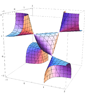
Figure 3: The allowed region for the three cross-ratios of null hexagons in four-dimensional Minkowski space. Points outside the central bag and the four ears are accessible only with null hexagons in $\mathbb{R}^{(2,2)}$.

In null hexagons with a self-crossing necessarily one of the $u_{i}$ equals one and the remaining two are equal to each other [9]. In the main text we have already noticed that a self-crossing situation with $pq>0$ can be reached only via $u_{i}\rightarrow 1-0$, which means from inside the central bag in fig.3. If $pq<0$ one can approach a self-crossing configuration only from inside the ears in fig.3.

As explained in the main text, the three cross-ratios do not uniquely fix the conformal class of the hexagon. While all self-crossing configurations have two equal cross-ratios and one equal to one, not all configurations with such a cross-ratio pattern are self-crossing. Clearly, self-crossing and not self-crossing configurations cannot be conformally mapped to each other.

To clarify how self-crossing configurations with diverging remainder function can be reached by continuous deformation from configurations without self-crossing, but with say $u_{2}=1,~{}~{}u=u_{1}=u_{3}$, we consider

$$x_{2} = (2,1,1,0),~{}~{}x_{3}~{}=~{}(2-\sqrt{b^{2}-2b+2},0,b,0),~{}~{}x_{4}~{}=~{}(2,-1,1,0)$$ (58)

$$x_{1} = (x_{10},\cos\psi,-1,\sin\psi),~{}~{}x_{5}=(x_{50},-\cos\psi,-1,-\sin\psi),~{}~{}x_{6}=(x_{60},0,-b,0),$$

with

$$x_{10}~{}=~{}x_{50}~{}=~{}2-\sqrt{6-2\cos\psi},~{}~{}x_{60}~{}=~{}2-\sqrt{6-2\cos\psi}+\sqrt{2+b^{2}-2b}~{}.$$ (59)

The related cross-ratios are

$$u_{2} = \frac{1}{\cos^{2}\psi}~{},$$

$$u = -~{}\frac{(~{}3-\cos\psi-2b-\sqrt{6-2\cos\psi}\sqrt{b^{2}-2b+2}~{})^{2}}{\cos\psi~{}(14-8b-2\cos\psi-4\sqrt{6-2\cos\psi}\sqrt{b^{2}-2b+2})}~{}.$$ (60)

For $\psi=0$ we have a not self-crossing hexagon with $u_{2}=1$ and for $\psi=\pi$ a self-crossing hexagon with again $u_{2}=1$. Their projections on the $(1,2)$-plane are shown in fig.4.

Figure 4: Projection to the (1,2)-plane of a null hexagon without self-crossing, but with $u_{2}=1$ (left) and after rotating $x_{1}$ and $x_{5}$ with angle $\pi$ in the (1,3)-plane (right).

The cross-ratio $u_{2}$ goes through infinity. Therefore, to follow the path of the cross-ratios for all $\psi\in(0,\pi)$, it is more convenient to consider its description in terms of $1/u$ and $1/u_{2}$. Then (60) results in a continuous and finite path in the $(1/u,1/u_{2})$-plane. Along the path $1/u_{2}$ goes from 1 to 0 and back to 1. For generic $b$ the initial and final values of $1/u$ differ, for the special case $b=-\frac{2(1+2\sqrt{2})}{7}=-1.094$ they agree.

The source for divergences in the analytic result of [5] are polylogarithms with argument $(1-\frac{1}{u_{i}})$. Now $(1-\frac{1}{u_{2}})$ for $\psi=0$ to $\psi=\pi$ goes from zero to one and back to zero. For the behaviour near one, where the polylogarithms have a branch point with a cut extending to $+\infty$, we have to remember that the $i\varepsilon$-prescription of the gluon propagator will take care for encircling the branch point. Let us handle the $(x_{j}-x_{k})^{2}$ factors in the cross-ratios in the same manner as the squared distances in the gluon propagator. Then we find, that the argument of the polylogarithms encircles the branch point at one in a counterclockwise (clockwise) manner for the standard (switched) $i\varepsilon$-prescription .

Appendix B

Renormalisation $Z$-factors are given as formal power series with terms $g^{2l}\epsilon^{-m}$ for dimensional regularisation and with terms $g^{2l}\log^{m}(\frac{1}{-z^{2}_{\perp}\mu^{2}})$ for a regularisation with a position space cutoff $z$ ($\mu$ RG-scale). In the case of correlation functions of local operators only terms with $m\leq l$ contribute. The complete all loop information on $\beta$-functions and anomalous dimensions is contained in the coefficients of the $m=1$ terms. On the other side, the coefficients of the terms with $m=l$ are fixed by one loop information and are independent of the renormalisation scheme.

In contrast to this situation, for polygonal Wilson loops with light-like edges also terms with $m>l$ appear. In dimensional regularisation the RG-scale enters exclusively in the combination $g^{2}\mu^{2\epsilon}$ and we have to deal with ($s$ some squared distance of polygon vertices)

$$g^{2l}~{}\frac{1}{\epsilon^{m}}(-\mu^{2}s)^{l\epsilon}~{}=~{}g^{2l}~{}\frac{1}{\epsilon^{m}}\left(1+\cdots+\frac{(l\epsilon)^{m-l}}{(m-l)!}~{}\log^{m-l}(-\mu^{2}s)+\cdots\right)~{}.$$ (61)

The analogous term in cutoff regularisation looks like

$$g^{2l}~{}\log^{m}(\frac{s}{z_{\perp}^{2}}) =g^{2l}~{}\Big{(}\log(-\mu^{2}s)+\log(\frac{1}{-\mu^{2}z_{\perp}^{2}})\Big{)}^{m}$$

$$=\cdots+g^{2l}~{}{m\choose l}\log^{m-l}(-\mu^{2}s)~{}\log^{l}\left(\frac{1}{-\mu^{2}z_{\perp}^{2}}\right)~{}+~{}\cdots$$ (62)

In both cases a term with $m>l$ generates descendents with lower powers of $\frac{1}{\epsilon}$ or $\log\frac{1}{-\mu^{2}z_{\perp}^{2}}$, respectively.
Now we assume the existence of some translation factor $\alpha$

$$g^{2l}~{}\frac{1}{\epsilon^{m}}(-\mu^{2}s)^{l\epsilon}~{}\Leftrightarrow~{}\alpha~{}g^{2l}~{}\log^{m}(\frac{s}{z_{\perp}^{2}})~{}.$$ (63)

Inserting in this correspondence (61) and (62) one finds, by comparison of the coefficients of $\log^{m-l}(-\mu^{2}s)$

$$g^{2l}\frac{1}{\epsilon^{l}}~{}\frac{l^{m-l}}{(m-l)!}~{}\Leftrightarrow~{}\alpha~{}g^{2l}\log^{l}\left(\frac{1}{-\mu^{2}z_{\perp}^{2}}\right){m\choose l}~{}.$$ (64)

Motivated by the scheme independence (for local operators) of factors in front of terms with equal powers of $g^{2}$ and $1/\epsilon$ or $\log(\frac{1}{-\mu^{2}z_{\perp}^{2}})$, we further assume that the translation factor $\alpha$ has to be chosen in such a manner that (64) becomes $g^{2l}/\epsilon^{l}\Leftrightarrow g^{2l}\log^{l}$. This fixes

$$\alpha~{}=~{}\frac{l^{m-l}~{}l!}{m!}~{}.$$ (65)

Looking then on the coefficients of $(\log(-\mu^{2}s))^{0}$ we get

$$g^{2l}~{}\frac{1}{\epsilon^{m}}~{}\Leftrightarrow~{}\alpha~{}g^{2l}~{}\log^{m}\left(\frac{1}{-\mu^{2}z_{\perp}^{2}}\right)~{},$$ (66)

with $\alpha$ from (65).

In particular this means
- at one loop    : $1/\epsilon^{2}~{}\Leftrightarrow~{}1/2~{}\log^{2}~{},~{}~{}1/\epsilon~{}\Leftrightarrow~{}\log$
- at two loops   : $1/\epsilon^{3}~{}\Leftrightarrow~{}2/3~{}\log^{3}~{},~{}~{}1/\epsilon^{2}~{}\Leftrightarrow~{}\log^{2}$
- at three loops : $1/\epsilon^{5}~{}\Leftrightarrow~{}9/20~{}\log^{5}~{},~{}~{}1/\epsilon^{4}~{}\Leftrightarrow~{}3/4~{}\log^{4}$
It is straightforward to prove at least the first statement by an explicit calculation. Two further independent checks are emphasized in the conclusions.

References

- [1] L. F. Alday and J. M. Maldacena, JHEP 0706 (2007) 064 [arXiv:0705.0303 [hep-th]]. L. F. Alday and J. Maldacena, JHEP 0711 (2007) 068 [arXiv:0710.1060 [hep-th]].
- [2] G. P. Korchemsky, J. M. Drummond and E. Sokatchev, Nucl. Phys. B 795 (2008) 385 [arXiv:0707.0243 [hep-th]]. A. Brandhuber, P. Heslop and G. Travaglini, Nucl. Phys. B 794 (2008) 231 [arXiv:0707.1153 [hep-th]]. J. M. Drummond, J. Henn, G. P. Korchemsky and E. Sokatchev, Nucl. Phys. B 795 (2008) 52 [arXiv:0709.2368 [hep-th]]. J. M. Drummond, J. Henn, G. P. Korchemsky and E. Sokatchev, Nucl. Phys. B 815 (2009) 142 [arXiv:0803.1466 [hep-th]].
- [3] C. Anastasiou, Z. Bern, L. J. Dixon and D. A. Kosower, Phys. Rev. Lett. 91 (2003) 251602 [arXiv:hep-th/0309040]. Z. Bern, L. J. Dixon and V. A. Smirnov, Phys. Rev. D 72 (2005) 085001 [arXiv:hep-th/0505205].
- [4] V. Del Duca, C. Duhr and V. A. Smirnov, JHEP 1005 (2010) 084 [arXiv:1003.1702 [hep-th]].
- [5] A. B. Goncharov, M. Spradlin, C. Vergu and A. Volovich, Phys. Rev. Lett. 105 (2010) 151605 [arXiv:1006.5703 [hep-th]].
- [6] V. Del Duca, C. Duhr and V. A. Smirnov, JHEP 1009 (2010) 015 [arXiv:1006.4127 [hep-th]].
- [7] S. Caron-Huot, JHEP 1112 (2011) 066 [arXiv:1105.5606 [hep-th]].
- [8] L. J. Dixon, J. M. Drummond and J. M. Henn, JHEP 1111 (2011) 023 [arXiv:1108.4461 [hep-th]].
- [9] G. Georgiou, JHEP 0909 (2009) 021 [arXiv:0904.4675 [hep-th]].
- [10] H. Dorn and S. Wuttke, JHEP 1105 (2011) 114 [arXiv:1104.2469 [hep-th]].
- [11] A. M. Polyakov, Nucl. Phys. B 164 (1980) 171.
-
[12]
R. A. Brandt, F. Neri and M. A. Sato,
Phys. Rev. D 24 (1981) 879.
R. A. Brandt, A. Gocksch, M. A. Sato and F. Neri, Phys. Rev. D 26 (1982) 3611. - [13] H. Dorn, Fortsch. Phys. 34 (1986) 11.
- [14] I. A. Korchemskaya and G. P. Korchemsky, Nucl. Phys. B 437 (1995) 127 [arXiv:hep-ph/9409446].
- [15] G. P. Korchemsky and A. V. Radyushkin, Nucl. Phys. B 283 (1987) 342.
- [16] I. A. Korchemskaya and G. P. Korchemsky, Phys. Lett. B 287, 169 (1992).
- [17] A. Brandhuber, P. Heslop, P. Katsaroumpas, D. Nguyen, B. Spence, M. Spradlin and G. Travaglini, JHEP 1007 (2010) 080 [arXiv:1004.2855 [hep-th]].
- [18] L. F. Alday, D. Gaiotto and J. Maldacena, JHEP 1109 (2011) 032. [arXiv:0911.4708 [hep-th]].
- [19] S. Caron-Huot and S. He, “Jumpstarting the all-loop S-matrix of planar N=4 super Yang-Mills,” arXiv:1112.1060 [hep-th].
- [20] J. G. M. Gatheral, Phys. Lett. B 133 (1983) 90. J. Frenkel and J. C. Taylor, Nucl. Phys. B 246 (1984) 231.