Enumerating fundamental normal surfaces:
Algorithms, experiments and invariants

Abstract

Computational knot theory and 3-manifold topology have seen significant breakthroughs in recent years, despite the fact that many key algorithms have complexity bounds that are exponential or greater. In this setting, experimentation is essential for understanding the limits of practicality, as well as for gauging the relative merits of competing algorithms.

In this paper we focus on normal surface theory, a key tool that appears throughout low-dimensional topology. Stepping beyond the well-studied problem of computing vertex normal surfaces (essentially extreme rays of a polyhedral cone), we turn our attention to the more complex task of computing fundamental normal surfaces (essentially an integral basis for such a cone). We develop, implement and experimentally compare a primal and a dual algorithm, both of which combine domain-specific techniques with classical Hilbert basis algorithms. Our experiments indicate that we can solve extremely large problems that were once though intractable. As a practical application of our techniques, we fill gaps from the KnotInfo database by computing 398 previously-unknown crosscap numbers of knots.

Keywords Computational topology, knot theory, normal surfaces, Hilbert basis, algorithms, crosscap number

1 Introduction

Efficient computation in knot theory and 3-manifold topology remains a significant challenge, with important implications for mathematical research in these fields.

Theoretically, many algorithms in these fields are highly complex and appear to be infeasibly slow. For instance, the algorithm to test whether two 3-manifolds are homeomorphic (topologically equivalent) has never been implemented, and explicit bounds on its running time have never been computed; see [33] for just some of some of its highly intricate components.

Practically, however, the right blend of topology, algorithms and heuristics can yield surprising results. Well known examples include the software packages SnapPea [20, 44], Regina [10], and the 3-Manifold Recogniser [34], which are extremely effective for solving geometric, decomposition and recognition problems. This is despite the fact that there are often no proofs to guarantee the efficiency (or in some cases even the termination) of the underlying algorithms.

Obtaining practical algorithms such as these—even without theoretical guarantees—is important for mathematicians. A striking example was the resolution after 30 years of Thurston’s long-standing question on the Weber-Seifert dodecahedral space [15], in part due to surprisingly effective heuristic improvements to an algorithm that had been known since the 1980s [28], and whose best theoretical complexity bound remains doubly-exponential even today [11].

This is a typical pattern: where theoretical bounds do exist in low-dimensional topology, they are often extremely large—sometimes exponential, sometimes tower-of-exponential—and they often bear little relation to practical running times. In this setting, experimentation plays two crucial roles:

• It is necessary for understanding the practical boundary between what is and is not feasible;

• It is essential when comparing competing algorithms, since algorithms with smaller theoretical bounds do not always performs better in practice.

In this paper we focus on algorithms that enumerate normal surfaces. Normal surfaces are ubiquitous in algorithmic 3-manifold topology and knot theory, which gives such algorithms widespread topological applications. We show one such application at the end of this paper, where we apply our techniques to compute previously-unknown invariants of knots.

The main idea of normal surface theory is to reduce difficult topological searches to discrete problems on integer points in rational cones [23, 33]. A typical topological algorithm that uses normal surfaces might run as follows:

• We present the input to our problem as a 3-manifold triangulation $\mathcal{T}$ (so, if the input is a knot, we triangulate the knot complement [23]), and we frame our topological problem as a search for some embedded surface in $\mathcal{T}$ with a particular property (e.g., for the unknot recognition problem we search for an embedded disc with non-trivial boundary [23]).

• We prove that we can restrict this search to normal surfaces in $\mathcal{T}$, which are properly embedded surfaces that intersect the tetrahedra of $\mathcal{T}$ in a well-behaved fashion. We encode normal surfaces arithmetically as integer points in the normal surface solution cone $\mathscr{C}$, which is a pointed rational cone in $\mathbb{R}^{7n}$ where $n$ is the number of tetrahedra in $\mathcal{T}$.

• We prove that there is a finite list $\mathscr{L}$ of points in this cone for which, if $\mathcal{T}$ has a surface with the desired property, then some such surface is described by a point in our list $\mathscr{L}$. The algorithm now builds the cone $\mathscr{C}$, constructs the finite list $\mathscr{L}$, rebuilds the corresponding surfaces, and tests each for the desired property.

For different topological algorithms, the list $\mathscr{L}$ takes on different forms:

1. For some algorithms, $\mathscr{L}$ contains the smallest integer point on each extremal ray of the cone $\mathscr{C}$. The corresponding surfaces are called vertex normal surfaces.

   Topological algorithms of this type include unknot recognition [22, 23], 3-sphere recognition [29, 39], connected sum decomposition [29], and Hakenness testing [28, 31].

2. For some algorithms, $\mathscr{L}$ is the Hilbert basis for the cone $\mathscr{C}$; that is, all integer points in $\mathscr{C}$ that cannot be expressed as a non-trivial sum of other integer points in $\mathscr{C}$. The corresponding surfaces are called fundamental normal surfaces.

   Algorithms of this type include JSJ decomposition [33], computing knot genus in arbitrary 3-manifolds [2, 40], computing the crosscap number of a knot [12], and determining which Dehn fillings of a knot complement are Haken [30].

3. For some algorithms, the list $\mathscr{L}$ is much larger again: typically one must first enumerate all fundamental normal surfaces, and then (often at great expense) extend this list in some way.

We emphasise that not all integer points in $\mathscr{C}$ correspond to normal surfaces: there are additional combinatorial constraints called the quadrilateral constraints that such points must satisfy. As a result, normal surfaces only represent a very small subset of the integer points in $\mathscr{C}$. This is a powerful observation that underpins much of this paper.

Enumerating vertex surfaces—case (i) above—is a “best case scenario”, and is now a well-studied problem with highly effective solutions [8, 13]. The running time remains exponential, but this is unavoidable since the output size is known to be exponential for some families of inputs [7, 14].

Enumerating fundamental surfaces—case (ii)—is now the next major step to be made in “practical” normal surface theory, and this is what we address in this paper. We emphasise that, because of the high dimensionality of the cone and the potential for super-exponentially many solutions [23], “out-of-the-box” Hilbert basis algorithms such as those found in the excellent software package Normaliz [3, 4] are impractically slow for all but the simplest inputs. Instead we must marry classical Hilbert basis algorithms with the structure and constraints of normal surface theory. The result of this marriage, as described in this paper, is the first practical software for enumerating fundamental normal surfaces.

It is widely noted that no one algorithm for Hilbert basis enumeration is superior in all settings [3, 19, 37]. For this reason, we develop and experimentally compare two algorithms, which at their core are based upon two modern Hilbert basis algorithms:

• Our primal algorithm draws upon the primal Hilbert basis algorithm described by Bruns, Ichim and Koch [3, 4]. In brief, we (i) enumerate all vertex normal surfaces; (ii) use these to build a piecewise-convex representation of the non-convex portion of $\mathscr{C}$ that satisfies the quadrilateral constraints; and then (iii) run the Bruns-Ichim-Koch algorithm over each convex piece and combine the results.

• Our dual algorithm is based on the dual Hilbert basis algorithm of Bruns and Ichim [3], based on earlier work by Pottier [38]. This is an inductive algorithm that generalises the double description method for enumerating extreme rays of a polyhedron [8, 21, 35]. Our algorithm closely follows the general Bruns-Ichim method, with an additional “filtering” step that enforces the quadrilateral constraints at each intermediate stage.

Through detailed experimentation over a census of 10,986 triangulations whose cones have up to 245 dimensions, we find that the primal algorithm is both faster and more consistent in performance. As well as comparing the primal and dual algorithms, we use our experiments to study the bottlenecks of the primal algorithm, and thereby identify avenues for future improvement.

As an illustration of its applicability, we use the primal algorithm to compute 398 previously-unknown crosscap numbers of knots. The crosscap number is a knot invariant that is related to, but offers distinct information from, the knot genus [18, 36]. There is still no general algorithm known for computing crosscap numbers, and our results go a significant way towards filling in the 2640 missing crosscap numbers from the online KnotInfo database of knot invariants.

All implementations use the freely-available software package Regina [5, 10], and the primal algorithm also incorporates portions of Normaliz 2.10.1. The primal and dual algorithms are now built directly into Regina, and the additional code for computing crosscap numbers can be downloaded from http://www.maths.uq.edu.au/~bab/code/.

2 Preliminaries

Here we give a very brief overview of triangulations and normal surfaces. In keeping with the focus of this paper, we concentrate on the algebraic formulation at the expense of geometric insight; for further information the reader is referred to the excellent summary in [23].

Throughout this paper, the input for a topological problem is a 3-manifold triangulation $\mathcal{T}$, built from $n$ tetrahedra by affinely identifying (or “gluing together”) some or all of the $4n$ tetrahedron faces in pairs so that the resulting topological space is a 3-manifold (possibly with boundary).

Such triangulations are more general than simplicial complexes: as a result of the face gluings, different edges of the same tetrahedron might be identified together, and likewise with vertices. Two faces of the same tetrahedron may even be glued together. This general definition allows us to express rich topological structures using few tetrahedra, which is important for computation.

A normal surface in $\mathcal{T}$ is a properly embedded surface that meets each tetrahedron in a (possibly empty) disjoint union of normal discs, each of which is a curvilinear triangle or quadrilateral. Each triangle separates one vertex of the tetrahedron from the others, and each quadrilateral separates two vertices from the others, as illustrated in Figure 1(a). Normal surfaces may be disconnected or empty.

(a) Examples of normal discs

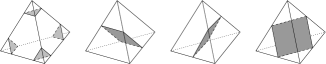
(b) The seven disc types in a tetrahedron

Figure 1: Normal triangles and quadrilaterals

There are seven types of disc in each tetrahedron, defined by which edges of the tetrahedron a normal disc meets. These include four triangle types and three quadrilateral types, all illustrated in Figure 1(b). The vector representation of a normal surface $S$ is a vector $\mathbf{v}(S)\in\mathbb{Z}^{7n}$, where the $7n$ elements of $\mathbf{v}(S)$ count the number of discs of each type in each tetrahedron. Given $\mathbf{v}(S)$, it is simple to reconstruct the surface $S$ (up to an isotopy that preserves the simplices of $\mathcal{T}$).

For each normal surface $S$, $\mathbf{v}(S)$ satisfies the matching equations. These are $3f$ linear homogeneous equations derived from $\mathcal{T}$, where $f$ is the number of non-boundary faces of $\mathcal{T}$. We express these equations as $A\cdot\mathbf{v}(S)=0$, where $A$ is a $3f\times 7n$ matching matrix. In essence, these equations ensure that triangles and quadrilaterals in adjacent tetrahedra can be joined together. The matching matrix $A$ is sparse with small integer entries. The normal surface solution cone $\mathscr{C}$ is the rational cone $\mathscr{C}=\{\mathbf{x}\in\mathbb{R}^{7n}\,|\,A\mathbf{x}=0,\ \mathbf{x}\geq 0\}$, which is a pointed cone with vertex at the origin.

No normal surface $S$ can have two different types of quadrilateral in the same tetrahedron, since these would necessarily intersect (contradicting the requirement that $S$ be properly embedded). We say that a vector $\mathbf{x}\in\mathbb{R}^{7n}$ satisfies the quadrilateral constraints if, for each tetrahedron $\Delta$ of $\mathcal{T}$, at most one of the three coordinates of $\mathbf{x}$ that counts quadrilaterals in $\Delta$ is non-zero. Running through all $n$ tetrahedra, this gives us $n$ distinct constraints of the form “at most one of $x_{i},x_{j},x_{k}$ is non-zero”. The quadrilateral constraints are non-linear, and their solution set is non-convex.

A point $\mathbf{x}\in\mathbb{R}^{7n}$ is called admissible if it lies in the cone $\mathscr{C}$ and satisfies the quadrilateral constraints. By a theorem of Haken [22], an integer vector $\mathbf{x}\in\mathbb{Z}^{7n}$ represents a normal surface if and only if $\mathbf{x}$ is admissible. The admissible region of $\mathscr{C}$ is the set of all admissible points in $\mathscr{C}$.

Let $\mathscr{P}\subset\mathbb{R}^{d}$ be any pointed rational cone with vertex at the origin, and let $\mathscr{P}\cap\mathbb{Z}^{d}$ denote all integer points in $\mathscr{P}$. Then the Hilbert basis of $\mathscr{P}\cap\mathbb{Z}^{d}$, denoted $\mathrm{Hilb}(\mathscr{P}\cap\mathbb{Z}^{d})$ or just $\mathrm{Hilb}(\mathscr{P})$ for convenience, is the minimal set of integer points that generates all of $\mathscr{P}\cap\mathbb{Z}^{d}$ under addition. Equivalently, $\mathrm{Hilb}(\mathscr{P})$ is the set of all $\mathbf{x}\in\mathscr{P}\cap\mathbb{Z}^{d}$ for which, if $\mathbf{x}=\mathbf{y}+\mathbf{z}$ with $\mathbf{y},\mathbf{z}\in\mathscr{P}\cap\mathbb{Z}^{d}$, then either $\mathbf{y}=0$ or $\mathbf{z}=0$. Hilbert bases are finite and unique [24, 43], and have many applications [17]. They can be defined more generally, but for this paper the definition above will suffice.

A fundamental normal surface is a normal surface $S$ for which, if $\mathbf{v}(S)=\mathbf{v}(T)+\mathbf{v}(U)$ for normal surfaces $T$ and $U$, then either $\mathbf{v}(T)=0$ or $\mathbf{v}(U)=0$. The fundamental normal surfaces are represented by the admissible points in $\mathrm{Hilb}(\mathscr{C})$, i.e., those points of $\mathrm{Hilb}(\mathscr{C})$ that satisfy the quadrilateral constraints.

A vertex normal surface is a normal surface $S$ for which $\mathbf{v}(S)$ lies on an extremal ray of $\mathscr{C}$ and the elements of $\mathbf{v}(S)$ have no common factor. It is clear that every vertex normal surface is also a fundamental normal surface, but in general the converse is not true.

3 The primal algorithm

We begin this section by outlining the primal algorithm described by Bruns, Ichim and Koch [3, 4] for enumerating Hilbert bases in general. Following this, we embed this into a larger algorithm tailored for enumerating fundamental surfaces that exploits the structure provided by normal surface theory.

The Bruns-Ichim-Koch algorithm comes in several forms [3, 4]; here we describe the variant most relevant to us. Let $\mathscr{P}\subset\mathbb{R}^{d}$ be a pointed rational cone with vertex at the origin. The Bruns-Ichim-Koch algorithm takes as input the extremal rays of $\mathscr{P}$, and computes the Hilbert basis $\mathrm{Hilb}(\mathscr{P})$. The following is an overview of the procedure; full details can be found in [3].

1. Use a variant of Fourier-Motzkin elimination to compute the supporting hyperplanes for $\mathscr{P}$, and triangulate $\mathscr{P}$ into simplicial subcones (cones whose extremal rays are linearly independent).

2. For each simplicial subcone $\mathscr{S}$, build the semi-open parallelotope spanned by the smallest integer vector on each extremal ray of $\mathscr{S}$, as shown in Figure 2(a). Specifically, if the extremal rays are defined by integer vectors $\mathbf{v}_{1},\ldots,\mathbf{v}_{k}$, we build the parallelotope $\{\sum\lambda_{i}\mathbf{v}_{i}\,|\,0\leq\lambda_{i}<1\}$.

   

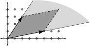
   (a) Building a semi-open parallelotope

   

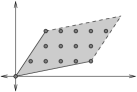
   (b) All integer points in the parallelotope

   Figure 2: Building parallelotopes in the primal algorithm

3. Identify all integer points within each semi-open parallelotope, as illustrated in Figure 2(b), and combine these into a single list, which generates all of $\mathscr{P}\cap\mathbb{Z}^{d}$. Reduce both the intermediate and final lists by removing redundant generators (i.e., vectors that can be expressed as non-trivial sums of others in the lists). The final reduced list is the Hilbert basis $\mathrm{Hilb}(\mathscr{P})$.

In our setting, we could run the Bruns-Ichim-Koch algorithm directly over the normal surface solution cone $\mathscr{C}\subset\mathbb{R}^{7n}$, but this is typically infeasible given the high dimensionality of $\mathscr{C}$. Moreover, it is wasteful: our aim is to enumerate fundamental normal surfaces, and so we do not need all of $\mathrm{Hilb}(\mathscr{C})$, but just its admissible points.

Our algorithm, instead of triangulating all of $\mathscr{C}$, triangulates only the (non-convex) admissible region of $\mathscr{C}$. We call a face $F\subseteq\mathscr{C}$ admissible if every point $\mathbf{x}\in F$ is admissible. In particular, note that the vertex normal surfaces correspond precisely to the admissible extremal rays of $\mathscr{C}$. A maximal admissible face of $\mathscr{C}$ is an admissible face that is not a strict subface of another admissible face.

One can show that the admissible region of $\mathscr{C}$ is precisely the union of all maximal admissible faces [9, 28]; in essence this decomposes the non-convex admissible region of $\mathscr{C}$ into a union of convex subcones. Note that maximal admissible faces may have different dimensions, and if we truncate the origin (which is common to all faces) then the admissible region may even be disconnected.

Our strategy is to enumerate all maximal admissible faces of $\mathscr{C}$, and then use the Bruns-Ichim-Koch algorithm to triangulate and compute the Hilbert basis for each. This has the advantage that maximal admissible faces are often significantly simpler than the full cone $\mathscr{C}$: they have lower dimension [9], and are often generated by very few admissible extremal rays [7]. This can significantly reduce the burden on the general Hilbert basis enumeration procedure. The overall algorithm is as follows:

Algorithm 1 (Primal algorithm for fundamental normal surfaces).

To enumerate all fundamental normal surfaces in a given triangulation:

1. Enumerate all vertex normal surfaces—that is, all admissible extremal rays of $\mathscr{C}$—using the algorithms in [6] and [13], which are optimised specifically for normal surface theory. Let $\mathcal{V}$ be the resulting set of admissible extremal rays.

2. Using $\mathcal{V}$ as input, enumerate all maximal admissible faces of $\mathscr{C}$ (see Algorithm 3 below).

3. For each maximal admissible face $F\subseteq\mathscr{C}$, identify which rays in $\mathcal{V}$ are subfaces of $F$, and pass these rays as input to the Bruns-Ichim-Koch algorithm which will then enumerate $\mathrm{Hilb}(F)$. The union $\bigcup\mathrm{Hilb}(F)$ over all maximal admissible faces $F$ is is precisely the set of all vector representations of fundamental normal surfaces.

The correctness of the algorithm follows from the following observation:

Lemma 2.

A vector $\mathbf{x}\in\mathbb{R}^{7n}$ represents a fundamental normal surface if and only if there is some maximal admissible face $F\subseteq\mathscr{C}$ for which $\mathbf{x}\in\mathrm{Hilb}(F)$.

Proof.

Let $\mathbf{x}=\mathbf{v}(S)$ where $S$ is a fundamental normal surface. Since $\mathbf{x}$ is an admissible point of $\mathscr{C}$, it must belong to some maximal admissible face $F\subseteq\mathscr{C}$. If $\mathbf{x}\notin\mathrm{Hilb}(F)$ then there are non-zero integer vectors $\mathbf{y},\mathbf{z}\in F$ for which $\mathbf{x}=\mathbf{y}+\mathbf{z}$. Since $F$ is an admissible face of $\mathscr{C}$ it follows that $\mathbf{y}=\mathbf{v}(T)$ and $\mathbf{z}=\mathbf{v}(U)$ for some normal surfaces $T$ and $U$, contradicting the fundamentality of $S$.

Conversely, suppose that $\mathbf{x}\in\mathrm{Hilb}(F)$ for some maximal admissible face $F\subseteq\mathscr{C}$. Then $\mathbf{x}$ is an admissible integer vector of $\mathscr{C}$, and so $\mathbf{x}=\mathbf{v}(S)$ for some normal surface $S$. If $S$ is not fundamental then $\mathbf{v}(S)=\mathbf{v}(T)+\mathbf{v}(U)$ for normal surfaces $T$ and $U$ with $\mathbf{v}(T),\mathbf{v}(U)\neq 0$. Since they represent normal surfaces, both $\mathbf{v}(T),\mathbf{v}(U)\in\mathscr{C}$, and so any face of the cone $\mathscr{C}$ that contains $\mathbf{v}(S)$ must contain both summands $\mathbf{v}(T)$ and $\mathbf{v}(U)$ as well. In particular we have $\mathbf{v}(T),\mathbf{v}(U)\in F$, contradicting the assumption that $\mathbf{x}=\mathbf{v}(T)+\mathbf{v}(U)\in\mathrm{Hilb}(F)$. ∎

In the remainder of this section we expand upon steps 2 and 3 of Algorithm 1.

We represent faces $F\subseteq\mathscr{C}$ using zero sets [21]. For each face $F\subseteq\mathscr{C}$, the zero set of $F$ is a subset of $\{1,\ldots,7n\}$ indicating which coordinate positions are zero throughout $F$. We denote this zero set by $Z(F)$, and define it formally as $Z(F)=\{k\,|\,x_{k}=0\ \mbox{for all}\ \mathbf{x}\in F\}$.

Because $\mathscr{C}$ is of the form $\{\mathbf{x}\in\mathbb{R}^{7n}\,|\,A\mathbf{x}=0,\ \mathbf{x}\geq 0\}$, zero sets effectively encode the support hyperplanes for each face: it is then clear that for any two faces $F,G\subseteq\mathscr{C}$ we have $Z(F)=Z(G)$ if and only if $F=G$, and $Z(F)\subseteq Z(G)$ if and only if $G\subseteq F$. Zero sets can be stored and manipulated efficiently in code using bitmasks of length $7n$.

The enumeration of maximal admissible faces makes use of admissible zero sets, which correspond to admissible faces of $\mathscr{C}$. We call a set $z\subseteq\{1,\ldots,7n\}$ admissible if the corresponding zero/non-zero coordinate pattern satisfies the quadrilateral constraints in $\mathbb{R}^{7n}$; that is, for each tetrahedron $\Delta$ of our triangulation, at most one of the three coordinate positions that counts quadrilaterals in $\Delta$ does not appear in $z$.

Algorithm 3 (Maximal admissible face decomposition).

Given the set $\mathcal{V}$ of all admissible extremal rays of $\mathscr{C}$, the following algorithm enumerates all maximal admissible faces of $\mathscr{C}$.

1. Build zero sets for all rays $R\in\mathcal{V}$ and store these in the set $\mathcal{S}_{1}$. Initialise an empty output set $\mathcal{M}$, which will eventually contain the zero sets for all maximal admissible faces of $\mathscr{C}$.

2. Inductively build sets $\mathcal{S}_{2},\mathcal{S}_{3},\ldots$ as follows. To build the set $\mathcal{S}_{k}$:

   1. For each zero set $z\in\mathcal{S}_{k-1}$, find all $v\in\mathcal{S}_{1}$ for which $z\nsubseteq v$ and $z\cap v$ is admissible. For each such $v$, insert $z\cap v$ into $\mathcal{S}_{k}$. If no such $v$ exists, insert $z$ into the output set $\mathcal{M}$.

   2. Reduce $\mathcal{S}_{k}$ to its maximal elements by set inclusion. That is, remove all $z\in\mathcal{S}_{k}$ for which there exists some strict superset $z^{\prime}\in\mathcal{S}_{k}$.

   3. If $\mathcal{S}_{k}$ is empty, terminate the algorithm and return the output set $\mathcal{M}$.

The key observation is that each set $\mathcal{S}_{i}$, once constructed, contains precisely the zero sets for all admissible faces of dimension $i$. A full proof of correctness and termination will be given shortly.

First, however, we make a simple observation regarding zero sets. Recall from standard polytope theory that, for any two faces $F$ and $G$ of a polyhedron $\mathscr{P}$, the join $F\vee G$ is the unique smallest-dimensional face of $\mathscr{P}$ that contains both $F$ and $G$, and that for any face $H\subseteq\mathscr{P}$ with $F,G\subseteq H$ we have $F\vee G\subseteq H$ [45].

Lemma 4.

For any two faces $F$ and $G$ of the normal surface solution cone $\mathscr{C}$, we have $Z(F\vee G)=Z(F)\cap Z(G)$.

Proof.

Since $F\vee G\supseteq F,G$, any coordinate position that takes a non-zero value in either $F$ or $G$ also takes a non-zero value somewhere in $F\vee G$. Therefore $Z(F\vee G)\subseteq Z(F)\cap Z(G)$.

Let $H$ be the face of $\mathscr{C}$ obtained by intersecting $\mathscr{C}$ with the supporting hyperplanes $\{x_{i}=0\}$ for all $i\in Z(F)\cap Z(G)$. It is clear that $Z(F)\cap Z(G)\subseteq Z(H)$. Moreover, $F,G\subseteq H$ since every point in $F$ or $G$ lies on all of the supporting hyperplanes listed above. Therefore $F\vee G\subseteq H$, and so $Z(F)\cap Z(G)\subseteq Z(H)\subseteq Z(F\vee G)$.

We now have $Z(F\vee G)\subseteq Z(F)\cap Z(G)\subseteq Z(F\vee G)$, and so $Z(F\vee G)=Z(F)\cap Z(G)$. ∎

We can now move on to the full proof of correctness and termination for Algorithm 3.

Proof of correctness and termination.

We first prove by induction that, once constructed, each set $\mathcal{S}_{i}$ contains precisely the zero sets for all admissible faces of $\mathscr{C}$ of dimension $i$.

This is clearly true for $i=1$, since the 1-dimensional faces of $\mathscr{C}$ are precisely the extremal rays, and we use all admissible extremal rays of $\mathscr{C}$ to fill $\mathcal{S}_{1}$ in step 1 of the algorithm.

Consider now some $i>1$. We assume our inductive hypothesis for both $\mathcal{S}_{i-1}$ and $\mathcal{S}_{1}$, and prove it for $\mathcal{S}_{i}$ in three stages:

1. Every $y\in\mathcal{S}_{i}$ is the zero set $Z(F)$ for some admissible face $F\subseteq\mathscr{C}$ of dimension $\geq i$.

   Suppose that $y$ is constructed in step 2(a) of the algorithm as $y=z\cap v$, where $z\in\mathcal{S}_{i-1}$ and $v\in\mathcal{S}_{1}$. By the inductive hypothesis we have $z=Z(G)$ and $v=z(R)$ for some admissible faces $G,R\subseteq\mathscr{C}$ with $\dim(G)=i-1$ and $\dim(R)=1$.

   By Lemma 4 we have $y=Z(G\vee R)$. Because step 2(a) of the algorithm only constructs admissible zero sets $y=z\cap v$, it follows that $G\vee R$ must be an admissible face. Because step 2(a) only considers pairs for which $z\nsubseteq v$, it follows that $R\nsubseteq G$ and therefore $G\vee R$ has strictly higher dimension than $G$; that is, $\dim(G\vee R)\geq i$.

2. For every admissible $i$-dimensional face $F\subseteq\mathscr{C}$, we have $Z(F)\in\mathcal{S}_{i}$.

   Let $G\subseteq F$ be any $(i-1)$-dimensional subface of $F$, and let $R\subseteq F$ be any extremal ray of $F$ not contained in $G$. Since $F\supseteq G,R$ we have $F\supseteq G\vee R$, and since $i-1=\dim(G)<\dim(G\vee R)\leq\dim(F)=i$ it follows that $\dim(F)=\dim(G\vee R)$, and hence $F=G\vee R$. By Lemma 4 we then have $Z(F)=Z(G)\cap Z(R)$.

   Since $F$ is admissible, so are $G$ and $R$, and it follows from the inductive hypothesis that $Z(G)\in\mathcal{S}_{i-1}$ and $Z(R)\in\mathcal{S}_{1}$. Because $R\nsubseteq G$ we have $Z(G)\nsubseteq Z(R)$, and we already know from $F$ that $Z(F)=Z(G)\cap Z(R)$ is admissible. Therefore the set $Z(F)=Z(G)\cap Z(R)$ is inserted into $\mathcal{S}_{i}$ in step 2(a) of the algorithm.

   Furthermore, $Z(F)$ is not removed from $\mathcal{S}_{i}$ in step 2(b) of the algorithm. This is because, by stage (i) above, any strict superset $z^{\prime}\supset Z(F)$ that appears in $\mathcal{S}_{i}$ must correspond to a strict subface $F^{\prime}\subset F$ of dimension $\geq i$. This is impossible, since $F$ itself has dimension $i$.

3. For every admissible $j$-dimensional face $F\subseteq\mathscr{C}$ with $j>i$, we have $Z(F)\notin\mathcal{S}_{i}$.

   For any such $F$, let $G\subseteq F$ be any $i$-dimensional subface of $F$. Because $F$ is admissible, $G$ is also, and by stage (ii) above it follows that $Z(G)\in\mathcal{S}_{i}$. Since $G$ is a strict subface of $F$, $Z(G)$ is a strict superset of $Z(F)$, and so even if $Z(F)$ is constructed in step 2(a) of the algorithm, it will be subsequently removed in step 2(b).

Together these three stages establish our inductive claim.

From here it is simple to see that Algorithm 3 terminates: since the cone $\mathscr{C}$ has finitely many faces, there are only finitely many non-empty sets $\mathcal{S}_{k}$. Note also that Algorithm 3 does not terminate until all non-empty sets $\mathcal{S}_{k}$ have been constructed, since if $\mathcal{S}_{k}$ is empty then there are no admissible $k$-faces, which means there can be no admissible $i$-faces for any $i\geq k$.

To finish, we show that the output of Algorithm 3 is correct. Let $F\subseteq\mathscr{C}$ be any maximal admissible face of dimension $i$; by our induction above we have $Z(F)\subseteq\mathcal{S}_{i}$. Suppose there is some $v\in\mathcal{S}_{1}$ for which $Z(F)\nsubseteq v$ and for which $Z(F)\cap v$ is admissible. Following the argument in stage (i) above, $Z(F)\cap v$ must be the zero set for some admissible face of dimension $\geq i+1$. Moreover, this must be a strict superface of $F$, which contradicts the maximality of $F$. Therefore there can be no such $v\in\mathcal{S}_{1}$, and so we include $Z(F)$ in the output set $\mathcal{M}$ as required.

Conversely, consider any output $z\in\mathcal{M}$. We must have $z\in\mathcal{S}_{i}$ for some $i$, and so $z=Z(G)$ for some admissible $i$-dimensional face $G\subseteq\mathscr{C}$. If $G$ is not maximal, there must be some admissible $(i+1)$-dimensional superface $F\supset G$, and some admissible extremal ray $R\subseteq F$ not contained in $G$. Following the argument in stage (ii) above, for the pair $Z(G)\in\mathcal{S}_{i}$ and $Z(R)\in\mathcal{S}_{1}$ we have $Z(G)\nsubseteq Z(R)$ and $Z(G)\cap Z(R)$ is admissible, which means we would not insert $z$ into the output set $\mathcal{M}$ in step 2(a) of the algorithm. Therefore $z=Z(G)$ for some maximal admissible face $G\subseteq\mathscr{C}$. ∎

In Algorithm 3, note that each zero set in step 1 can be built by examining any non-zero representative of the corresponding ray $R$. In step 2(a), a set might be constructed from many different $(z,v)$ pairs, and so it is important when inserting $z\cap v$ into $\mathcal{S}_{k}$ to avoid duplicates. Each $\mathcal{S}_{k}$ is only required for the following inductive step (building $\mathcal{S}_{k+1}$), and can then be discarded.

Returning to Algorithm 1, in step 3 we can use zero sets to quickly identify which rays are subfaces of $F$: a ray $R\in\mathcal{V}$ is a subface of $F$ if and only if $Z(R)\supseteq Z(F)$. The Bruns-Ichim-Koch algorithm does enumerate $\mathrm{Hilb}(F)$ as described, since each extremal ray of $F$ is admissible, and so the rays in $\mathcal{V}$ that are subfaces of $F$ (which we give Bruns-Ichim-Koch as input) are indeed the extremal rays of $F$.

4 The dual algorithm

We now outline the dual algorithm of Bruns and Ichim [3] for general Hilbert basis enumeration, which is based on earlier work of Pottier [38], and then show how this can be seamlessly modified to yield a dual algorithm for enumerating fundamental normal surfaces.

The Bruns-Ichim-Pottier dual algorithm has several variants, and we describe the variant most relevant to us. Consider the cone $\mathscr{P}=\{\mathbf{x}\in\mathbb{R}^{d}\,|\,A\mathbf{x}=0,\ \mathbf{x}\geq 0\}$, where $A$ is some rational $m\times d$ matrix. The dual algorithm takes as input the matrix $A$, and computes the Hilbert basis $\mathrm{Hilb}(\mathscr{P})$.

It constructs a series of cones $\mathscr{P}^{(0)},\ldots,\mathscr{P}^{(m)}$, beginning with the non-negative orthant $\mathscr{P}^{(0)}=\mathbb{R}^{d}_{\geq 0}$, and finishing with the target cone $\mathscr{P}^{(m)}=\mathscr{P}$. In general, $\mathscr{P}^{(k)}$ is defined as for $\mathscr{P}$ above but using only the first $k$ rows of the matrix $A$. At each stage, the dual algorithm uses the previous basis $\mathrm{Hilb}(\mathscr{P}^{(k-1)})$ to inductively compute the next basis $\mathrm{Hilb}(\mathscr{P}^{(k)})$. In this sense, the dual algorithm generalises the double description method for enumerating extremal rays [21, 35].

The key inductive step of the dual algorithm is the following [3].

Algorithm 5 (Bruns-Ichim-Pottier inductive step).

Let $\mathscr{P}\subset\mathbb{R}^{d}$ be a pointed rational cone with vertex at the origin, let $\mathbf{h}\in\mathbb{R}^{d}$ be a rational vector, and define the cones $\mathscr{P}_{+}=\{\mathbf{x}\in\mathscr{P}\,|\,\mathbf{h}\cdot\mathbf{x}\geq 0\}$, $\mathscr{P}_{-}=\{\mathbf{x}\in\mathscr{P}\,|\,\mathbf{h}\cdot\mathbf{x}\leq 0\}$, and $\mathscr{P}_{0}=\{\mathbf{x}\in\mathscr{P}\,|\,\mathbf{h}\cdot\mathbf{x}=0\}$. Then, given the input basis $B=\mathrm{Hilb}(\mathscr{P})$, the following algorithm computes the Hilbert bases $\mathrm{Hilb}(\mathscr{P}_{+})$, $\mathrm{Hilb}(\mathscr{P}_{-})$ and $\mathrm{Hilb}(\mathscr{P}_{0})$.

1. Initialise candidate bases $B_{+}=\{\mathbf{x}\in B\,|\,\mathbf{h}\cdot\mathbf{x}\geq 0\}$ and $B_{-}=\{\mathbf{x}\in B\,|\,\mathbf{h}\cdot\mathbf{x}\leq 0\}$.

2. Expand these candidate bases: for all pairs $\mathbf{x}\in B_{+}$ and $\mathbf{y}\in B_{-}$ with $\mathbf{h}\cdot\mathbf{x}>0>\mathbf{h}\cdot\mathbf{y}$, insert the sum $\mathbf{x}+\mathbf{y}$ into $B_{+}$ and/or $B_{-}$ according to whether $\mathbf{h}\cdot(\mathbf{x}+\mathbf{y})\geq 0$ and/or $\mathbf{h}\cdot(\mathbf{x}+\mathbf{y})\leq 0$.

3. Reduce the candidate bases: remove all $\mathbf{b}\in B_{+}$ for which there exists some different $\mathbf{b}^{\prime}\in B_{+}$ with $\mathbf{b}-\mathbf{b}^{\prime}\in\mathscr{P}_{+}$. Reduce $B_{-}$ in a similar fashion.

4. If $B_{+}$ and $B_{-}$ are both unchanged after the most recent round of expansion and reduction (steps 2 and 3), terminate with $\mathrm{Hilb}(\mathscr{P}_{+})=B_{+}$, $\mathrm{Hilb}(\mathscr{P}_{-})=B_{-}$, and $\mathrm{Hilb}(\mathscr{P}_{0})=B_{+}\cap B_{-}$. Otherwise return to step 2 for a new round of expansion and reduction.

In essence, step 2 expands the set of integer points that are generated under addition by each individual set $B_{+}$ and $B_{-}$, and step 3 removes redundant vectors from each generating set. See [3] for full proofs of correctness and termination, both of which are non-trivial results.

There are many ways to optimise this algorithm. In practice, one can split $B_{+}$ and $B_{-}$ into three sets according to whether $\mathbf{h}\cdot\mathbf{x}>0$, $\mathbf{h}\cdot\mathbf{x}<0$ or $\mathbf{h}\cdot\mathbf{x}=0$, to avoid duplication along the common hyperplane $\mathbf{h}\cdot\mathbf{x}=0$. The expansion and reduction steps can be partially merged, so that we first test each new sum $\mathbf{x}+\mathbf{y}$ for reduction before inserting it into $B_{+}$ and/or $B_{-}$. Several other optimisations are possible: see [3, Remark 16], and the “darwinistic reduction” in [3, Section 3].

As with the primal method, running the dual algorithm of Bruns, Ichim and Pottier directly over the normal surface solution cone $\mathscr{C}\subset\mathbb{R}^{7n}$ can be extremely slow. Like the double description method for vertex enumeration, one significant problem is combinatorial explosion: even if the final Hilbert basis $\mathrm{Hilb}(\mathscr{P})$ is small, the intermediate bases $\mathrm{Hilb}(\mathscr{P}^{(k)})$ can be extremely large. The high dimension of the normal surface solution cone $\mathscr{C}$ exacerbates this problem.

Our solution, as with the primal algorithm, is to restrict our attention to just the admissible region of $\mathscr{C}$. This time we do not decompose the admissible region into maximal admissible faces; instead we can embed the quadrilateral constraints seamlessly into the algorithm itself. In this way, a single run through the dual algorithm can compute all admissible Hilbert basis elements for $\mathscr{C}$.

The idea is simple: when expanding candidate bases, ignore sums $\mathbf{x}+\mathbf{y}$ that do not satisfy the quadrilateral constraints. This mirrors Letscher’s filter for the double description method [8].

Algorithm 6 (Dual algorithm for fundamental normal surfaces).

To enumerate all fundamental normal surfaces in a triangulation with the $3f\times 7n$ matching matrix $A$:

1. Reorder the rows of $A$ using a good heuristic (as discussed further below).

2. Initialise the candidate basis $B^{(0)}$ with all unit vectors in $\mathbb{R}^{7n}$.

3. Inductively construct candidate bases $B^{(1)},\ldots,B^{(3f)}$ as follows. For each $i=1,\ldots,3f$, run a modified Algorithm 5 with input basis $B^{(i-1)}$, using the vector $\mathbf{h}\in\mathbb{R}^{7n}$ defined by the $i$th row of $A$. The specific modifications to Algorithm 5 are:

   • In step 2, only consider pairs $\mathbf{x},\mathbf{y}$ for which $\mathbf{x}+\mathbf{y}$ satisfies the quadrilateral constraints.

   • In step 3, instead of testing for $\mathbf{b}-\mathbf{b}^{\prime}\in\mathscr{P}_{+}$, test for $\mathbf{b}-\mathbf{b}^{\prime}\geq 0$ and $\mathbf{h}\cdot(\mathbf{b}-\mathbf{b}^{\prime})\geq 0$. Instead of testing for $\mathbf{b}-\mathbf{b}^{\prime}\in\mathscr{P}_{-}$, test for $\mathbf{b}-\mathbf{b}^{\prime}\geq 0$ and $\mathbf{h}\cdot(\mathbf{b}-\mathbf{b}^{\prime})\leq 0$.

   When this modified Algorithm 5 terminates with output $B_{+}$ and $B_{-}$, set $B^{(i)}=B_{+}\cap B_{-}$.

4. The final set $B^{(3f)}$ is then the set of all vector representations of fundamental normal surfaces.

Although we use the Bruns-Ichim-Pottier inductive process in step 3 of our algorithm, we never identify any explicit cone $\mathscr{P}\subset R^{7n}$ for which the input set $B^{(i-1)}$ is the Hilbert basis (this is because we only ever track admissible basis elements). This is why we modify step 3 of Algorithm 5: we must remove any reference to the unknown cone $\mathscr{P}$.

The key invariant in this dual algorithm is that each candidate basis $B^{(i)}$ contains precisely those Hilbert basis elements for the cone defined by the first $i$ rows of the matching matrix $A$ that satisfy the quadrilateral constraints. See the appendix for full proofs of correctness and termination.

The order in which we process the rows of $A$ can have a significant effect on performance, by affecting the severity of the combinatorial explosion [3, 21]. In step 1 of Algorithm 6, we reorder the rows using position vectors [8], which essentially favours rows that begin with long strings of zeroes. Position vectors help optimise our quadrilateral constraint filter, and have been found to perform well as a sorting heuristic for the related double description method; see [8] for details.

We can prove correctness and termination for Algorithm 6 as follows.

Proof of correctness and termination.

Let $A^{(k)}$ denote the $k\times 7n$ submatrix of $A$ obtained by taking the first $k$ rows (after the reordering in step 1 of the algorithm), and let $\mathscr{P}^{(k)}=\{\mathbf{x}\in\mathbb{R}^{7n}\,|\,A^{(k)}\mathbf{x}=0,\ \mathbf{x}\geq 0\}$. We prove by induction that each candidate basis $B^{(k)}$ constructed in Algorithm 6 consists of all elements of $\mathrm{Hilb}(\mathscr{P}^{(k)})$ that satisfy the quadrilateral constraints.

The initial case is simple: $\mathscr{P}^{(0)}$ is just the non-negative orthant $\mathbb{R}^{7n}_{\geq 0}$, whose Hilbert basis consists of the unit vectors in $\mathbb{R}^{7n}$, all of which satisfy the quadrilateral constraints. This matches the initialisation of $B^{(0)}$ in step 2 of the algorithm.

Assume now that $B^{(i-1)}$ contains all elements of $\mathrm{Hilb}(\mathscr{P}^{(i-1)})$ that satisfy the quadrilateral constraints, and consider the construction of $B^{(i)}$ in step 3 of Algorithm 6. This involves running a modified Algorithm 5 (the Bruns-Ichim-Pottier inductive step), with input basis $B^{(i-1)}$ and with the vector $\mathbf{h}\in\mathbb{R}^{7n}$ defined by the $i$th row of the (sorted) matrix $A$.

Let $\mathscr{P}_{+}=\{\mathbf{x}\in\mathscr{P}^{(i-1)}\,|\,\mathbf{h}\cdot\mathbf{x}\geq 0\}$, $\mathscr{P}_{-}=\{\mathbf{x}\in\mathscr{P}^{(i-1)}\,|\,\mathbf{h}\cdot\mathbf{x}\leq 0\}$, and $\mathscr{P}_{0}=\mathscr{P}_{+}\cap\mathscr{P}_{-}=\{\mathbf{x}\in\mathscr{P}^{(i-1)}\,|\,\allowbreak\mathbf{h}\cdot\mathbf{x}=0\}$. We claim that the modified Algorithm 5 terminates with output sets $B_{+}$ and $B_{-}$ containing those elements of $\mathrm{Hilb}(\mathscr{P}_{+})$ and $\mathrm{Hilb}(\mathscr{P}_{-})$ respectively that satisfy the quadrilateral constraints. If this is true, then setting $B^{(i)}=B_{+}\cap B_{-}$ will fill $B^{(i)}$ with those elements of $\mathrm{Hilb}(\mathscr{P}_{0})=\mathrm{Hilb}(\mathscr{P}^{(i)})$ that satisfy the quadrilateral constraints, as required. This will complete our induction, and the final output $B^{(3f)}$ will then consist of all admissible elements of $\mathrm{Hilb}(\mathscr{P}^{(3f)})=\mathrm{Hilb}(\mathscr{C})$; that is, all vector representations of fundamental normal surfaces.

It remains to prove our claim above, i.e., that the modified Algorithm 5 terminates with output sets $B_{+}$ and $B_{-}$ containing those elements of $\mathrm{Hilb}(\mathscr{P}_{+})$ and $\mathrm{Hilb}(\mathscr{P}_{-})$ respectively that satisfy the quadrilateral constraints.

Consider running the modified Algorithm 5 and the original Algorithm 5 side-by-side, where in the original algorithm we use the full basis $\mathrm{Hilb}(\mathscr{P}^{(i-1)})$ as input. Let $B_{+}^{m}$ and $B_{-}^{m}$ denote the working sets $B_{+}$ and $B_{-}$ in our modified algorithm, and let $B_{+}^{o}$ and $B_{-}^{o}$ denote the working sets $B_{+}$ and $B_{-}$ in the original algorithm. From Bruns and Ichim [3], we know that the original algorithm terminates with $B_{+}^{o}=\mathrm{Hilb}(\mathscr{P}_{+})$ and $B_{-}^{o}=\mathrm{Hilb}(\mathscr{P}_{-})$.

We claim that, for as long as both algorithms are running side-by-side, the working sets $B_{+}^{m}$ and $B_{-}^{m}$ contain precisely those elements of $B_{+}^{o}$ and $B_{-}^{o}$ respectively that satisfy the quadrilateral constraints. We show this again using induction:

• It is true when the algorithms begin, since we assume from our “outer induction” on $B^{(i)}$ that the input basis $B^{(i-1)}$ for the modified algorithm contains precisely those elements that satisfy the quadrilateral constraints from the input basis $\mathrm{Hilb}(\mathscr{P}^{(i-1)})$ for the original algorithm.

• We now show that, if at some point $B_{+}^{m}$ and $B_{-}^{m}$ contain the elements of $B_{+}^{o}$ and $B_{-}^{o}$ that satisfy the quadrilateral constraints, then this remains true after a single round of expansion (step 2 of Algorithm 5).

  It is clear from our modification in step 3 of Algorithm 6 that we do not insert any new sums $\mathbf{x}+\mathbf{y}$ into $B_{+}^{m}$ or $B_{-}^{m}$ that break the quadrilateral constraints. Moreover, in the original algorithm, any sum $\mathbf{x}+\mathbf{y}$ that does satisfy the quadrilateral constraints must have summands $\mathbf{x}\in B_{+}^{o}$ and $\mathbf{y}\in B_{-}^{o}$ that satisfy them also (since $\mathbf{x},\mathbf{y}\geq 0$); therefore $\mathbf{x}\in B_{+}^{m}$ and $\mathbf{y}\in B_{-}^{m}$, and the sum $\mathbf{x}+\mathbf{y}$ is also considered in the modified algorithm.

• Likewise, we can show that if at some point $B_{+}^{m}$ and $B_{-}^{m}$ contain the elements of $B_{+}^{o}$ and $B_{-}^{o}$ that satisfy the quadrilateral constraints, then this remains true after a single round of reduction (step 3 of Algorithm 5).

  First, we note that our modification to the reduction step is sound: for any $\mathbf{b},\mathbf{b}^{\prime}\in B_{+}^{m}$, we have $\mathbf{b}-\mathbf{b}^{\prime}\in\mathscr{P}_{+}$ if and only if $\mathbf{b}-\mathbf{b}^{\prime}\geq 0$ and $\mathbf{h}\cdot(\mathbf{b}-\mathbf{b}^{\prime})\geq 0$, since we already have $A^{(i-1)}\mathbf{b}=A^{(i-1)}\mathbf{b}^{\prime}=0$ from our outer induction. Next, we observe that a vector $\mathbf{b}\in B_{+}^{m}$ is removed in step 3 of the modified Algorithm 5 if and only if it is removed in the original algorithm: this is because $\mathbf{b}$ satisfies the quadrilateral constraints, and so any $\mathbf{b}^{\prime}$ for which $\mathbf{b}-\mathbf{b}^{\prime}\geq 0$ must satisfy them also, and therefore $\mathbf{b}^{\prime}\in B_{+}^{m}$ if and only if $\mathbf{b}^{\prime}\in B_{+}^{o}$. Similar arguments apply to $\mathscr{P}_{-}$ and $B_{-}^{m}$.

By induction, $B_{+}^{m}$ and $B_{-}^{m}$ contain precisely those elements of $B_{+}^{o}$ and $B_{-}^{o}$ that satisfy the quadrilateral constraints for as long as both algorithms are running.

It follows that the modified algorithm terminates no later than the original algorithm, since if $B_{+}^{o}$ and $B_{-}^{o}$ are unchanged under some round of expansion and reduction, then their elements $B_{+}^{m}$ and $B_{-}^{m}$ that satisfy the quadrilateral constraints are unchanged also. The modified algorithm might terminate earlier, but this will not change the final output: if $B_{+}^{m}$ and $B_{-}^{m}$ are unchanged under some earlier round of expansion and reduction, then running any additional rounds will leave them unchanged.

Either way, we see that the final output sets $B_{+}^{m}$ and $B_{-}^{m}$ from the modified Algorithm 5 contain precisely those elements of the final output sets $B_{+}^{o}=\mathrm{Hilb}(\mathscr{P}_{+})$ and $B_{-}^{o}=\mathrm{Hilb}(\mathscr{P}_{-})$ that satisfy the quadrilateral constraints, thus establishing our original claim. ∎

5 Experimentation

For our experiments, we implement both the primal and dual algorithms directly in the software package Regina [5, 10]. The primal algorithm uses the tree traversal method [13] for step 1 (enumerating vertex surfaces), and calls Normaliz 2.10.1 [3, 4] for step 3 (the Bruns-Ichim-Koch algorithm). The dual algorithm incorporates optimisations described by Bruns and Ichim [3]. All implementations use arbitrary-precision integer arithmetic.

Our experimental data set is the closed hyperbolic census of Hodgson and Weeks [26], which consists of 10,986 3-manifold triangulations with sizes from $n=9$ to $n=35$ tetrahedra. This census was chosen because (i) it contains “real-world” triangulations with properties and structures that one might encounter in a typical topological algorithm; and (ii) the triangulations are large enough to make the problems difficult and the results mathematically interesting.

The triangulations were sorted by increasing $n$, and then each algorithm was run over the census on a cluster, processing triangulations in parallel until a fixed walltime limit was reached. For the primal algorithm, the limit was 4 days walltime with 15 slave processes (each of which could process one triangulation at a time). For the dual algorithm it became clear early on that the results would be severely limited (as discussed below), and so it was rerun with 4 days walltime and 31 slave processes to increase the number of triangulations for which the two algorithms could be compared. All processes ran on 2.93GHz Intel Xeon X5570 CPUs.

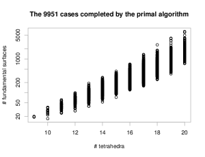
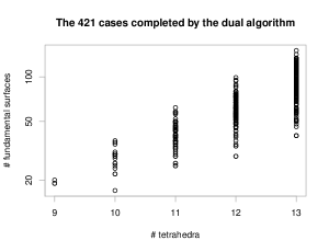
Figure 3: Input and output sizes for test cases that were completed

The primal algorithm completed 9951 of the 10986 test cases, and the dual algorithm completed just 421. Figure 3 summarises the input and output sizes for these cases, with output size on a log scale. Figure 4 compares running times for the 421 cases that were completed by both algorithms (there were no cases that the dual algorithm completed but the primal algorithm did not). Each point on the plot represents an individual triangulation, and here both axes use log scales.

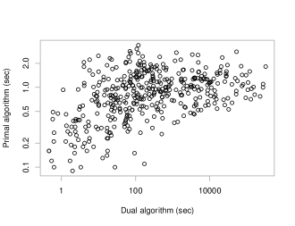
Figure 4: Comparison of running times for the cases solved by both algorithms

It is clear from the figure that the primal algorithm runs significantly faster. This contrasts with the enumeration of vertex normal surfaces, where the corresponding double description is fast for problems of this size (but becomes inferior when the problems become larger) [13]. The primal method is also more consistent in its performance: for $n=13$ (the largest amongst these 421 cases), the primal algorithm ranges from $0.44$ to $3.36$ seconds (spanning a single order of magnitude), whereas the dual algorithm ranges from $4.02$ to $322\,544$ seconds (spanning five orders of magnitude).

We now drill more deeply into the primal algorithm, to find where its bottlenecks lie. For this we use all 9951 cases that it completed, so that we can study how the algorithm behaves for larger and more difficult problems. Figure 5 shows how the running time is divided amongst the three main steps of (i) enumerating vertex surfaces; (ii) constructing maximal admissible faces; and (iii) running the Bruns-Ichim-Koch algorithm over each. For each plot, the horizontal axis measures total running time (on a log scale), as an indicator of how difficult overall each test case was found to be.

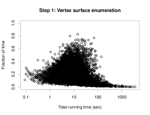
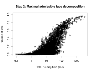
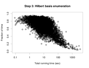
Figure 5: Division of time for the primal algorithm

We see that, as the running time grows, it is the enumeration of maximal admissible faces that consumes the bulk of the running time. Significant gains could therefore be made by incorporating more sophisticated algorithms and data structures into this step. One promising approach could be to adapt the Kaibel-Pfetsch algorithm for general polytopes [32] to the setting of normal surface theory.

6 Application to crosscap numbers

To illustrate the practicality of the primal algorithm, we use it to compute previously-unknown crosscap numbers of knots. Related to the genus of a knot, the crosscap number $C(K)$ of a knot $K$ is an invariant describing the smallest-genus non-orientable surface that the knot bounds.

Crosscap numbers are difficult to compute: of the 2977 non-trivial prime knots with $\leq 12$ crossings, 2640 crosscap numbers are still unknown (in contrast, the genus is known for all of these knots) [16]. Although there are specialised methods for certain classes of knots [1, 25, 27, 41], there is no algorithm known for computing crosscap numbers in general. However, we can come close: by enumerating fundamental normal surfaces, it is possible to either compute the crosscap number of a knot precisely or else reduce it to one of two possible values [12].

Due to space limitations we only give a very brief summary of the computational results here. See [12] for more information on crosscap numbers and the underlying algorithm.

The crosscap number algorithm [12, Algorithm 4.4] works with triangulated knot complements: these are triangulated 3-manifolds with boundary, obtained by removing a small regular neighbourhood of a knot from the 3-sphere. The algorithm requires the triangulation $\mathcal{T}$ to have specific properties (an “efficient suitable triangulation”), which can be tested by enumerating vertex normal surfaces. It then enumerates all fundamental normal surfaces in $\mathcal{T}$, runs some simple tests over each (such as whether the knot bounds the surface, and computing the orientable or non-orientable genus), and then either determines $C(K)$ precisely or declares that $C(K)\in\{t,t+1\}$ for some $t$.

We process our knot complements in order by increasing number of tetrahedra, and stop at the point where the computations become infeasibly slow; our longest computation ran for $1.61$ days. In total, we were able to run the algorithm over 585 knots, whose number of tetrahedra $n$ ranged from 5 to 27 (mean and median $n\simeq 22.7$ and $24$). The mean and median running times were $\simeq 258$ and $\simeq 52$ minutes respectively, which is extremely pleasing given that these enumeration problems involve up to $7\times 27=189$ dimensions. When this crosscap number algorithm was developed [12], such computations were believed to be beyond practical possibility for all but the very simplest of knots.

The final outcomes are also pleasing. We are able to compute 398 of the unknown crosscap numbers precisely, which goes a significant way towards filling in the 2640 missing crosscap numbers from the KnotInfo database. For the remaining 187 calculations that completed, we obtain information that is already known. All results, both new and known, are consistent with exiting KnotInfo data. A detailed table of results can be found at http://www.maths.uq.edu.au/~bab/code/.

It should be noted that the paper [12] also computes new crosscap numbers, but using integer programming methods instead. Our techniques here require knots whose complements do not have too many tetrahedra; in contrast, the integer programming techniques of [12] can work with very large knot complements, but only where good lower bounds on $C(K)$ are already known. In this sense, the two methods complement each other well.

Benjamin A. Burton
School of Mathematics and Physics, The University of Queensland
Brisbane QLD 4072, Australia
(bab@maths.uq.edu.au)

References

- [1] Colin Adams and Thomas Kindred, A classification of spanning surfaces for alternating links, Preprint, arXiv:1205.5520, May 2012.
- [2] Ian Agol, Joel Hass, and William Thurston, 3-manifold knot genus is NP-complete, STOC ’02: Proceedings of the Thiry-Fourth Annual ACM Symposium on Theory of Computing, ACM Press, 2002, pp. 761–766.
- [3] Winfried Bruns and Bogdan Ichim, Normaliz: Algorithms for affine monoids and rational cones, J. Algebra 324 (2010), no. 5, 1098–1113.
- [4] Winfried Bruns and Robert Koch, Computing the integral closure of an affine semigroup, Univ. Iagel. Acta Math. (2001), no. 39, 59–70, Effective methods in algebraic and analytic geometry, 2000 (Kraków).
- [5] Benjamin A. Burton, Introducing Regina, the 3-manifold topology software, Experiment. Math. 13 (2004), no. 3, 267–272.
- [6] , Converting between quadrilateral and standard solution sets in normal surface theory, Algebr. Geom. Topol. 9 (2009), no. 4, 2121–2174.
- [7] , The complexity of the normal surface solution space, SCG ’10: Proceedings of the Twenty-Sixth Annual Symposium on Computational Geometry, ACM, 2010, pp. 201–209.
- [8] , Optimizing the double description method for normal surface enumeration, Math. Comp. 79 (2010), no. 269, 453–484.
- [9] , Maximal admissible faces and asymptotic bounds for the normal surface solution space, J. Combin. Theory Ser. A 118 (2011), no. 4, 1410–1435.
- [10] Benjamin A. Burton, Ryan Budney, William Pettersson, et al., Regina: Software for 3-manifold topology and normal surface theory, http://regina.sourceforge.net/, 1999–2013.
- [11] Benjamin A. Burton, Alexander Coward, and Stephan Tillmann, Computing closed essential surfaces in knot complements, SCG ’13: Proceedings of the 29th Annual Symposium on Computational Geometry, ACM, 2013, pp. 405–414.
- [12] Benjamin A. Burton and Melih Ozlen, Computing the crosscap number of a knot using integer programming and normal surfaces, ACM Trans. Math. Software 39 (2012), no. 1, 4:1–4:18.
- [13] , A tree traversal algorithm for decision problems in knot theory and 3-manifold topology, Algorithmica 65 (2013), no. 4, 772–801.
- [14] Benjamin A. Burton, João Paixão, and Jonathan Spreer, Computational topology and normal surfaces: Theoretical and experimental complexity bounds, ALENEX 2013: Proceedings of the Meeting on Algorithm Engineering & Experiments, SIAM, 2013, pp. 78–87.
- [15] Benjamin A. Burton, J. Hyam Rubinstein, and Stephan Tillmann, The Weber-Seifert dodecahedral space is non-Haken, Trans. Amer. Math. Soc. 364 (2012), no. 2, 911–932.
- [16] Jae Choon Cha and Charles Livingston, KnotInfo: Table of knot invariants, http://www.indiana.edu/~knotinfo, accessed September 2013.
- [17] D. Chubarov and A. Voronkov, Basis of solutions for a system of linear inequalities in integers: Computation and applications, Mathematical Foundations of Computer Science 2005, Lecture Notes in Comput. Sci., vol. 3618, Springer, Berlin, 2005, pp. 260–270.
- [18] Bradd Evans Clark, Crosscaps and knots, Internat. J. Math. Math. Sci. 1 (1978), no. 1, 113–123.
- [19] Evelyne Contejean and Hervé Devie, An efficient incremental algorithm for solving systems of linear Diophantine equations, Inform. and Comput. 113 (1994), no. 1, 143–172.
- [20] Marc Culler, Nathan M. Dunfield, and Jeffrey R. Weeks, SnapPy, a computer program for studying the geometry and topology of 3-manifolds, http://snappy.computop.org/, 1991–2011.
- [21] Komei Fukuda and Alain Prodon, Double description method revisited, Combinatorics and Computer Science (Brest, 1995), Lecture Notes in Comput. Sci., vol. 1120, Springer, Berlin, 1996, pp. 91–111.
- [22] Wolfgang Haken, Theorie der Normalflächen, Acta Math. 105 (1961), 245–375.
- [23] Joel Hass, Jeffrey C. Lagarias, and Nicholas Pippenger, The computational complexity of knot and link problems, J. Assoc. Comput. Mach. 46 (1999), no. 2, 185–211.
- [24] David Hilbert, Ueber die Endlichkeit des Invariantensystems für binäre Grundformen, Math. Ann. 33 (1888), no. 2, 223–226.
- [25] Mikami Hirasawa and Masakazu Teragaito, Crosscap numbers of 2-bridge knots, Topology 45 (2006), no. 3, 513–530.
- [26] Craig D. Hodgson and Jeffrey R. Weeks, Symmetries, isometries and length spectra of closed hyperbolic three-manifolds, Experiment. Math. 3 (1994), no. 4, 261–274.
- [27] Kazuhiro Ichihara and Shigeru Mizushima, Crosscap numbers of pretzel knots, Topology Appl. 157 (2010), no. 1, 193–201.
- [28] William Jaco and Ulrich Oertel, An algorithm to decide if a -manifold is a Haken manifold, Topology 23 (1984), no. 2, 195–209.
- [29] William Jaco and J. Hyam Rubinstein, 0-efficient triangulations of 3-manifolds, J. Differential Geom. 65 (2003), no. 1, 61–168.
- [30] William Jaco and Eric Sedgwick, Decision problems in the space of Dehn fillings, Topology 42 (2003), no. 4, 845–906.
- [31] William Jaco and Jeffrey L. Tollefson, Algorithms for the complete decomposition of a closed -manifold, Illinois J. Math. 39 (1995), no. 3, 358–406.
- [32] Volker Kaibel and Marc E. Pfetsch, Computing the face lattice of a polytope from its vertex-facet incidences, Comput. Geom. 23 (2002), no. 3, 281–290.
- [33] Sergei Matveev, Algorithmic topology and classification of 3-manifolds, Algorithms and Computation in Mathematics, no. 9, Springer, Berlin, 2003.
- [34] Sergei Matveev et al., Manifold recognizer, http://www.matlas.math.csu.ru/?page=recognizer, accessed August 2012.
- [35] T. S. Motzkin, H. Raiffa, G. L. Thompson, and R. M. Thrall, The double description method, Contributions to the Theory of Games, Vol. II (H. W. Kuhn and A. W. Tucker, eds.), Annals of Mathematics Studies, no. 28, Princeton University Press, Princeton, NJ, 1953, pp. 51–73.
- [36] Hitoshi Murakami and Akira Yasuhara, Crosscap number of a knot, Pacific J. Math. 171 (1995), no. 1, 261–273.
- [37] Dmitrii V. Pasechnik, On computing Hilbert bases via the Elliot-MacMahon algorithm, Theoret. Comput. Sci. 263 (2001), no. 1-2, 37–46, Combinatorics and computer science (Palaiseau, 1997).
- [38] Loïc Pottier, The Euclidean algorithm in dimension , ISSAC ’96: Proceedings of the 1996 International Symposium on Symbolic and Algebraic Computation, ACM, 1996, pp. 40–42.
- [39] J. Hyam Rubinstein, An algorithm to recognize the -sphere, Proceedings of the International Congress of Mathematicians (Zürich, 1994), vol. 1, Birkhäuser, 1995, pp. 601–611.
- [40] Horst Schubert, Bestimmung der Primfaktorzerlegung von Verkettungen, Math. Z. 76 (1961), 116–148.
- [41] Masakazu Teragaito, Crosscap numbers of torus knots, Topology Appl. 138 (2004), no. 1-3, 219–238.
- [42] Jeffrey L. Tollefson, Normal surface -theory, Pacific J. Math. 183 (1998), no. 2, 359–374.
- [43] J. G. van der Corput, Über systeme von linear-homogenen Gleichungen und Ungleichungen, Proc. Kon. Ned. Akad. Wetensch. 34 (1931), 368–371.
- [44] Jeffrey R. Weeks, SnapPea: Hyperbolic 3-manifold software, http://www.geometrygames.org/SnapPea/, 1991–2000.
- [45] Günter M. Ziegler, Lectures on polytopes, Graduate Texts in Mathematics, no. 152, Springer-Verlag, New York, 1995.