A space–time varying coefficient model: The equity of service accessibility

Abstract

Research in examining the equity of service accessibility has emerged as economic and social equity advocates recognized that where people live influences their opportunities for economic development, access to quality health care and political participation. In this research paper service accessibility equity is concerned with where and when services have been and are accessed by different groups of people, identified by location or underlying socioeconomic variables. Using new statistical methods for modeling spatial-temporal data, this paper estimates demographic association patterns to financial service accessibility varying over a large geographic area (Georgia) and over a period of 13 years. The underlying model is a space–time varying coefficient model including both separable space and time varying coefficients and space–time interaction terms. The model is extended to a multilevel response where the varying coefficients account for both the within- and between-variability. We introduce an inference procedure for assessing the shape of the varying regression coefficients using confidence bands.

T1Supported in part by the NSF Grant CMMI-0954283 and by the industry research Georgia Tech foundation gift provided by Predictix.

1 Introduction

“A home is more than a shelter—when located in a community with resources and amenities it is a critical determinant of opportunity.” [Blackwell and Fox (2004)]

Service accessibility equity is the study of systematic disparities in a population’s access to services that are considered fundamental in fostering economic development, improving wellness and enhancing the general quality of life of a population within a given geographic area. Examples of such services are health care, education, healthy food, financial services and others. Accessibility is measured as utilization-scaled travel cost of a community $U$ to the nearby sites in a service network consisting of multiple service sites geographically distributed: ${\cal S}=\{s_{1},\ldots,s_{n}\}$. A common utilization measure is the population rate within the community and its surroundings [Marsh and Schilling (1994)]. In this paper the utilization is measured as the population rate divided by the service rate to account for the service availability for each population unit.

One challenge in measuring service accessibility is defining the travel cost for the residents in a community to access the sites in the service network. In the research works so far, the travel cost is calculated as the average or minimum distance between the centroid of the region $U$ and the nearby sites in the service network [Lovett et al. (2002); Talen (1997); Talen (2001)]. However, communities occupy uneven geographic areas varying in size, and, therefore, their simplified representation by their centroids is restrictive. In this research paper, we instead represent a community by a sample of locations in the neighborhood $U$, $u_{1},\ldots,u_{B}\in U$, and compute the street-network distances from these sample locations to the service network. Furthermore, the travel cost at each sample location $u_{b}$ is measured as a summary of the travel distances, $\{d(u_{b},s_{i})\}_{i=1,\ldots,n}$.

Combining the two ideas discussed above, utilization-adjustment of the travel cost and representation of a community by a series of sample spatial points, we evaluate the accessibility of a neighborhood to a service network in year $t$ using

$$Y(U,t)=\frac{1}{B}\sum_{b=1}^{B}(C(u_{b},t)^{\beta}W(u_{b},t)),$$ (1)

where $C(u_{b},t)$ is the travel cost at the sample location $u_{b}$ measured as the average street-network distance to the closest $Q$ service sites available at time $t$ (in our study, $Q=3$), $W(u_{b},t)$ is the utilization adjustment factor at location $u_{b}$ and $\beta$ is a distance utility parameter. We estimate $\beta$ by robust linear regression: $\log(W(u_{b},t))\sim-\log(C(u_{b},t))$.

Dividing the geographic space into contiguous spatial units $U_{\!s},s\,{=}\,1,\ldots,S$, where each spatial unit corresponds to a neighborhood (e.g., census tract), the accessibility measure (utilization-adjusted travel cost) varies across the geographic space and time; $Y(U_{s},t)=Y(s,t)$ defines the space–time varying accessibility process. Moreover, there are multiple providers in the service network, the accessibility process has an intrinsic multilevel structure. Under this multilevel structure, let $Y_{p}(s,t)$ be the accessibility of the community $U_{s}$ to the sites of the $p$th provider for $p=1,\ldots,P$, where $P$ is the number of service providers.

This research paper focuses on measuring and estimating spatial-temporal patterns in the association between demographic variables (including race, ethnicity and income) and service accessibility. Specific questions that will be addressed within this study are as follows: Is service accessibility equitable across population groups varying in ethnicity and income? Do service distribution inequities vary across regions and time? Are there service providers that provide a more equitable distribution of their services than others? What is the most common demographic feature associated with inequities?

To evaluate the equity of service accessibility with respect to various population groups over a period of time and within a large geographic space, we propose to estimate the space–time varying association of the accessibility measure jointly over a series of demographic variables. In this context, weak associations or the absence of systematic disparities in service access are interpreted as service accessibility equity. One challenge of this association analysis is simultaneous estimation of the association patterns since the goal is to assess both the equity with respect to various ethnicity and race demographic variables controlling for income and the equity with respect to income controlling for ethnicity and race. A second challenge is that services are delivered within a multilevel network - multiple providers which deliver across multiple service sites.

Many existing studies have analyzed service accessibility for different groups of people identified by underlying socioeconomic variables, but they are limited to small geographic areas and to only one year of data [Graves (2003); Larson (2003); Powell et al. (2007); Small and McDermott (2006); Talen (2001); Talen and Anselin (1998); Zenk et al. (2005)]. Commonly employed statistical procedures include regression methods assuming independence between service sites. Exploratory studies rely on graphical diagnostics but not on statistical inference, which can be used to make informed decisions. Although the methods applied to the existing studies have usefulness for some research questions, a spatial-temporal multivariate analysis of data with a multilevel structure requires new statistical methods which are rigorous, take into account the dependence in the data, and implementable, apply to real data complexity.

To this end, we introduce a space–time (multilevel) model which allows estimation of space–time varying association patterns of a set of functional predictors (e.g., demographic variables) to a functional response, in our case study, the accessibility process. The modeling procedure introduced in this paper falls under a more general framework: varying-coefficient models. These models have been applied to longitudinal data to estimate time-dependent effects on a response variable [Assuncao (2003); Fan and Zhang (2000); Hastie and Tibshirani (1993); Hoover et al. (1998); Huang, Wu and Zhou (2002); Wu and Liang (2004); Zhang (2004)]. Waller et al. (2007) review existing models to explore space-varying regressions and propose a Bayesian procedure. Gelfand et al. (2003) briefly mention the extension of their proposed Bayesian space-varying model to separable space–time varying coefficient models with a warning on its computational challenges. Space–time separability greatly simplifies the problem by reducing the computational effort; however, it is a restrictive assumption since it implies that dependence attenuates in a multiplicative/additive manner across space and time. Therefore, extension of the Bayesian varying coefficient model to more complex modeling (e.g., space–time interaction) requires expensive computations which may be prohibitive for densely sampled spatial domains.

Our methodological contribution is three-fold. First, we propose a space–time varying coefficient model that takes into account the interaction between time and space in a computationally efficient manner. To overcome the computational complexity due to operations with a large dependence matrix, we use a low-rank approximation to the space–time coefficient processes using radial basis of functions [Ruppert, Wand and Carroll (2003)]; this approach enables estimation of the space–time varying coefficient model for densely observed space and/or time domains.

Second, we extend this model to multilevel data, resulting in a multilevel varying coefficient model. A few recent works have considered the study of multilevel functional models [Baladandayuthapani et al. (2008); Crainiceanu, Staicu and Di (2009); Di et al. (2009); Morris and Carroll (2006); Morris et al. (2003); Rice and Wu (2001); Staicu, Crainiceanu and Carroll (2010); Wu and Zhang (2002)]. In the related research, models of multilevel functional data have been applied to functional responses where the predictor is a fixed variate, commonly time, and, more recently, they have been extended to functional predictors but scalar responses. In this paper, the multilevel functional model applies to both functional response and functional predictors and it extends to the more difficult setting when the functionality is with respect to space and time. Challenges in estimating such a complex model include nonidentifiability and computational efficiency. We overcome the identifiability problem by using a knots-based kernel decomposition with a different set of knots across the model coefficients. We use penalized splines for computational efficiency in adapting to the smoothness in the space–time varying coefficients [Ruppert, Wand and Carroll (2003)].

Third, we introduce an inference procedure to assess the shape of the space–time varying coefficients. Generally, a common approach for identifying the shape of a regression function is hypothesis testing. However, for our model, hypothesis testing will require multiple tests for deciding whether its shape is nonlinear, linear or constant as a function of space or/and time. In this paper, we discuss an inference procedure for assessing the shape of the varying regression coefficients using confidence bands.

The rest of the paper is organized as follows. In Sections 2 and 3 we present the space–time varying coefficient model as well as its extension to multilevel data along with the estimation and inference procedures. In Section 4 we present the application of the models introduced in this paper to evaluate the equity of financial service accessibility in Georgia. We first describe the data resources followed by the discussion of our results and findings. Section 5 concludes the paper. Some technical details are deferred to the supplemental material [Serban (2011)], which also provides complemental graphical descriptions of our analysis of the equity of service accessibility.

2 Space–time varying coefficient model

2.1 The model

In this section we introduce a space–time varying coefficient model for estimating the relationships between the accessibility process and a series of demographic variables varying in time and space. The observed data are $(Y_{ij},\{X_{r,ij},r=1,\ldots,R\})$, where $Y_{ij}=Y(t_{i},s_{j})$ is the response variable and $X_{r,ij}=X_{r}(t_{i},s_{j})$ a set of covariates observed at location $s_{j}=(s_{j1},s_{j2})$, $j=1,\ldots,S$, and time $t_{i},i=1,\ldots,T$, such that $\mathbb{E}[Y_{ij}|X]=\gamma_{1}(t_{i},s_{j})X_{1,ij}+\cdots+\gamma_{R}(t_{i},s_{j})X_{R,ij}$ where $\gamma_{r}(t,s)$ for $r=1,\ldots,R$ are smooth coefficient functions. Note that not all covariates need to vary in both time and space; the modeling procedure allows for various predictor forms (scalar, varying in time, varying in space or both). For example, in our model implementation we take $X_{1,ij}=1$ and, therefore, $\gamma_{1}(s,t)$ is the intercept coefficient.

In this paper we decompose the regression coefficients into separable space and time global effects along with space–time deviations from the global effects which are intrinsically local and account for the interaction between space and time:

$$\gamma_{r}(t,s)=\alpha_{r}(t)+\beta_{r}(s)+\sum_{m=1}^{M_{r}}\sum_{n=1}^{N_{r}}\nu_{r,mn}K_{\mathrm{temp}}\bigl{(}\bigl{|}t-\kappa^{(T)}_{m}\bigr{|}\bigr{)}K_{sp}\bigl{(}\bigl{\|}s-\kappa^{(S)}_{n}\bigr{\|}\bigr{)}.$$

We decompose the global coefficient functions using the radial spline basis [Ruppert, Wand and Carroll (2003)],

$$\alpha_{r}(t) = \tau_{r,0}+\tau_{r,1}t+\sum_{m=1}^{M_{r}}u_{r,m}K_{\mathrm{temp}}\bigl{(}\bigl{|}t-\kappa^{(T)}_{m}\bigr{|}\bigr{)},$$ (2)

$$\beta_{r}(s_{1},s_{2}) = \delta_{r,0}+\delta_{r,11}s_{1}+\delta_{r,12}s_{2}+\sum_{n=1}^{N_{r}}v_{r,n}K_{sp}\bigl{(}\bigl{\|}s-\kappa^{(S)}_{n}\bigr{\|}\bigr{)}.$$ (3)

In these decompositions $K_{\mathrm{temp}}(t)$ is a temporal kernel whereas $\kappa^{(T)}_{m}$, $m=1,\ldots,M_{r}$, are knots covering the time domain, and $K_{sp}(s)$ is a spatial kernel whereas $\kappa^{(S)}_{n}$, $n=1,\ldots,N_{r}$, are knots covering the space domain.

Importantly, although the kernel of the space–time interaction coefficient is separable in time and space, the decomposition is not. One advantage of using this kernel decomposition is that it allows decomposition of the design matrix as a Kronecker product, which, in turn, will ease the computations in the estimation procedure. We derive the Kronecker product decomposition in the Supplemental Material 1 of this paper.

In the semiparametric literature a common kernel function is the radial spline kernel function defined for $d$-dimensional domains [Nychka and Saltzman (1998)]. Bivariate smoothing based on radial basis functions has the advantage of being rotational invariant, which is important in geographical smoothing. For two-dimensional domains, the function $K_{sp}(\cdot)$ could be replaced by any other covariance function [Cressie (1993)], for example, the Matérn covariance function.

Knots for one-dimensional spaces are commonly set to the sample quantiles of the observation points, whereas knots for two-dimensional spaces are commonly selected using the space-filling algorithm [Nychka and Saltzman (1998)], which is based on minimax design, or $k$-nearest neighbor clustering algorithms. In this paper we implement these standard methods to select the number of knots.

2.2 Estimation

We choose a method for estimating the model described in the previous section from among several candidate procedures. One modeling approach is smoothing splines [Wahba (1990)], which assumes that the number of knots is equal to the number of observation design points ($M_{r}=T$ and $N_{r}=S$) and controls the smoothness of the coefficient by penalizing the influence of the coefficients $u_{r,m},m=1,\ldots,M_{r}$, and $v_{r,n},n=1,\ldots,N_{r}$, using a penalty function. One primary drawback of this estimation procedure is its computational aspect. A less computational approach is regression splines [Wahba (1990)], in which a small number of knots are used ($M_{r}\ll T$ and $N_{r}\ll S$). This reduces to selection of the optimal numbers of knots, which can be computationally expensive in the context of our model since it requires solving a multidimensional optimization problem. The smoothness levels of the regression functions differ from one covariate to another and, therefore, we need to optimally identify $(M_{r},N_{r})s$ for $r=1,\ldots,R$. In addition, this approach introduces modeling bias.

An alternative approach to optimal knots selection is to assume equal number of spatial knots ($N_{r}=N$ for $r=1,\ldots,R$) and equal number of temporal knots ($M_{r}=M$ for $r=1,\ldots,R$) with $N$ and $M$ sufficiently large such that the modeling bias is small [Li and Ruppert (2008)], but, similarly to smoothing splines, impose constraints on the coefficients $u_{r,m}$, $v_{r,n}$, and $\nu_{r,nm}$ as follows:

$$\sum_{m=1}^{M}u_{r,m}^{2}\leq C_{r}^{(T)},\qquad\sum_{n=1}^{N}v_{r,n}^{2}\leq C_{r}^{(S)},\qquad\sum_{m=1}^{M}\sum_{n=1}^{N}\nu_{r,mn}^{2}\leq C_{r}$$

or, equivalently, estimate the coefficients using penalized regression

$$\|h(Y_{k,ij})-\gamma_{1}(t_{i},s_{j})X_{1,ij}-\cdots-\gamma_{r}(t_{i},s_{j})X_{r,ij}\|^{2}$$

$$\qquad{}+\sum_{r=1}^{R}\bigl{\{}\lambda_{r}^{(T)}\mathbf{u}_{r}\mathbf{u}_{r}^{\prime}+\lambda_{r}^{(S)}\mathbf{v}_{r}\mathbf{v}_{r}^{\prime}+\lambda_{r}\bolds\nu_{r}\bolds\nu_{r}^{\prime}\bigr{\}},$$

where

$$\mathbf{u}_{r} = (u_{r,1},\ldots,u_{r,N}),\qquad\mathbf{v}_{r}=(v_{r,1},\ldots,v_{r,M})\quad\mbox{and }$$

$$\bolds\nu_{r} = \{\nu_{r,nm}\}_{n=1,\ldots,N,m=1,\ldots,M}.$$

Moreover, the parameters $\lambda_{r}^{(T)}$, $\lambda_{r}^{(S)}$ and $\lambda_{r}$ are penalties controlling the smoothness level of the regression coefficients. This approach is often referred to as penalized splines [Ruppert, Wand and Carroll (2003)]. Consequently, selection of the number of knots reduces to selection of the penalty parameters, which, in turn, is a multidimensional optimization problem.

In the semiparametric regression literature the problem of selecting the penalties, and implicitly of the the number of knots, is overcome by solving an equivalent mixed effects regression problem where $\mathbf{u}_{r}$, $\mathbf{v}_{r}$ and $\bolds\nu_{r}$ are random effects, specifically, $\mathbf{u}_{r}\sim N(0,(\sigma_{r}^{(T)})^{2}I_{n})$, $\mathbf{v}_{r}\sim N(0,(\sigma_{r}^{(S)})^{2}I_{m})$ and $\bolds\nu_{r}\sim N(0,\sigma_{r}^{2}I_{nm})$. Under the mixed effects model, the penalties are

$$\lambda_{r}^{(T)}=\frac{\sigma_{\varepsilon}^{2}}{(\sigma_{r}^{(T)})^{2}},\qquad\lambda_{r}^{(S)}=\frac{\sigma_{\varepsilon}^{2}}{(\sigma_{r}^{(S)})^{2}}\quad\mbox{and}\quad\lambda_{r}=\frac{\sigma_{\varepsilon}^{2}}{\sigma_{r}^{2}}.$$

We therefore estimate the model parameters using a mixed effects model to circumvent the difficulty of selecting the penalty parameters, or, implicitly, the number of knots.

Based on the mixed-effects model formulation, denote the vector of the fixed effects

$$\bolds\Theta=\left[\matrix{\tau_{1,0}&\tau_{1,1}&\delta_{1,0}&\delta_{1,11}&\delta_{1,12}&\cdots&\tau_{R,0}&\tau_{R,1}&\delta_{R,0}&\delta_{R,11}&\delta_{R,12}}\right]$$

with identifiability constraints $\delta_{r,0}=0$ for $r=1,\ldots,R$. The vector of random effects is

$$\mathbf{U}=\left[\matrix{\mathbf{u}_{1}&\mathbf{v}_{1}&\bolds\nu_{1}&\cdots&\mathbf{u}_{R}&\mathbf{v}_{R}&\bolds\nu_{R}}\right].$$

The corresponding design matrices ${\cal X}$ and ${\cal Z}$ are

$${\cal X} = \left[\matrix{\mathbf{X}_{1}(t_{i},s_{j})&\cdots&\mathbf{X}_{R}(t_{i},s_{j})}\right]_{i=1,\ldots,T,j=1,\ldots,S}$$

$$\eqntext{\mbox{with }\mathbf{X}_{r}(t_{i},s_{j})=X_{r}(t_{i},s_{j})\left[\matrix{1&t_{i}&1&s_{1j}&s_{2j}}\right],}$$ (4)

$${\cal Z} = \left[\matrix{\mathbf{Z}_{1}(t_{i},s_{j})&\cdots&\mathbf{Z}_{R}(t_{i},s_{j})}\right]_{i=1,\ldots,T,j=1,\ldots,S}$$

$$\eqntext{\mbox{with }\mathbf{Z}_{r}(t_{i},s_{j})=X_{r}(t_{i},s_{j})\left[\matrix{K_{\mathrm{temp}}\bigl{(}\bigl{|}t_{i}-\kappa^{(T)}_{m}\bigr{|}\bigr{)}&K_{sp}\bigl{(}\bigl{\|}s_{i}-\kappa^{(S)}_{n}\bigr{\|}\bigr{)}\hphantom{ii}}\right.}$$ (5)

$$\eqntext{\left.\matrix{K_{\mathrm{temp}}\bigl{(}\bigl{|}t_{i}-\kappa^{(T)}_{m}\bigr{|}\bigr{)}&K_{sp}\bigl{(}\bigl{\|}s_{i}-\kappa^{(S)}_{n}\bigr{\|}\bigr{)}}\right].}$$ (6)

The model in the matrix form becomes $\mathbb{E}[Y|{\cal X}]={\cal X}\bolds\Theta+{\cal Z}\mathbf{U}$, which is equivalent to a linear mixed model.

2.3 Inference

In this section we discuss alternative methods for making inference on the shape of the regression coefficients entering the space–time varying coefficient model described in Section 2.1. Specifically, we discuss a procedure for evaluating the shape (constant vs. linear vs. nonlinear) of the temporal and spatial global coefficients and a procedure for testing the significance of the space–time interaction.

Shape evaluation. In this section we discuss a novel procedure for shape evaluation of the temporal regression coefficients. A similar procedure applies to spatial regression coefficients. Specifically, each temporal regression coefficient can take various shapes, for example, constant [$\alpha(t)=\tau_{0}$], linear [$\alpha(t)=\tau_{0}+\tau_{1}t$] or nonlinear.

In varying-coefficient models, the common procedure for assessing the shape of the coefficients is hypothesis testing. For example, the hypothesis test for linearity is equivalent to $H_{0}\dvtx\sigma^{2}_{u}=0\mbox{ vs. }H_{a}\dvtx\sigma^{2}_{u}>0$ where $\sigma_{u}^{2}$ is the variance of the random effects $u_{m}$ under the mixed effects model. The common approach is a likelihood ratio testing (LRT) procedure. Crainiceanu et al. (2005) developed a LRT by taking advantage of the existing research in hypothesis testing for zero variance in linear mixed-effects (LME) models. Liang, Wu and Carroll (2003) tested for linearity of nonparametric functions using a Crámer–von Mises statistic.

Although there are several competitive approaches for testing for linearity of the regression coefficients, because we need to test sequential hypotheses to decide about the shape of a coefficient and because we often have a large number of predictors that enter the space–time varying coefficient model, we instead propose identifying the shape of the coefficients using simultaneous confidence bands. If $CB_{\gamma}$ is a $1-\gamma$ confidence band for the coefficient $\alpha(t)$, then $P(\alpha(t)\in CB_{\gamma},t\in{\cal T})\geq 1-\gamma$ where ${\cal T}$ is the time domain. The derivation of the joint confidence bands is presented in the Supplemental Material 2 of this paper.

Many authors have noted that using confidence intervals has a series of advantages over the conventional hypothesis testing [Sim and Reid (1999)]. Confidence intervals cannot only be used to test a hypothesis, but also to provide additional information on the variability of an observed sample statistic and on its probable relationship to the value of this statistic in the population from which the sample was drawn.

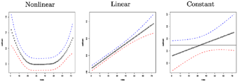
Figure 1: Examples of nonlinear, linear, constant effects.

Figure 1 depicts examples of three different one-dimensional shapes along with their confidence bands (CB). We define “constant” shape if there exists a constant line that falls within the confidence bands. Similarly, we define “linear” shape if there exists a linear function that falls within the confidence bands. When searching for a line $L$ within the confidence bands, it suffices to search for linear functions between the convex hull of the upper level of the confidence band and the convex hull of the lower level of the confidence band. Although the coverage of the shape test hypothesis is maintained when using confidence bands, the power may be reduced, as we point out in the simulation study included in Supplemental Material 4.

According to the result below, accepting the null hypothesis at a significance level $\gamma$ is equivalent to finding at least one null shape function in the set of all possible functions in the $(1-\gamma)$ confidence band.

Proposition 1.

Denote $\Theta_{c}=\{\alpha(t)\dvtx\alpha(t)=c,c\in\mathbb{R}\}$ (the set of all real constant functions). The rejection rule of the hypothesis test for constant shape ($H_{0}\dvtx\alpha(t)\in\Theta_{c}$) becomes

$$\Theta_{c}\cap CB_{\gamma}=\varnothing\qquad\mbox{where }P\bigl{(}\alpha(t)\in CB_{\gamma}\bigr{)}=1-\gamma.$$

Using this rejection rule, the type I error is equal to $\gamma$.

This proposition follows from the classical result on the equivalence of confidence intervals and hypothesis testing in Lehmann (1997).

Space–time interaction. In our modeling approach, in order to account for the space–time interaction, we introduce an additional term in $\gamma_{r}(t,s)$ specified by a set of effects $\bolds\nu_{r}=\{\nu_{r,nm}\}_{n=1,\ldots,N,m=1,\ldots,M}$. The testing procedure for space–time interaction of the regression coefficient for the $r$th predictor reduces to

$$H_{0}\dvtx\sigma_{\nu_{r}}=0\quad\mbox{vs.}\quad H_{0}\dvtx\sigma_{\nu_{r}}>0.$$

The null hypothesis implies that the association between the $r$th predictor and the response is separable in time and space.

Although there are several approaches for testing the null hypothesis of zero variance component in linear mixed effects models, hypothesis tests that apply under multiple variance components have been investigated only recently. To test for space–time interaction under a multiple predictor model, we therefore use the approximations to the finite sample null distribution of the RLRT statistic in Greven et al. (2008).

3 Multilevel varying coefficient model

In this section we discuss the extension of the varying-coefficient model in Section 2 to data with an intrinsic multilevel structure.

3.1 The model

The observed data for the $p$th category (e.g., service provider) for $p=1,\ldots,P$ are $(Y_{p,ij},X_{r,ij})$, where $Y_{p,ij}=Y_{p}(t_{i},s_{j})$ is a generalized response variable and $X_{r,ij}=X_{r}(t_{i},s_{j})$ the $r$th covariate observed at location $s_{j}=(s_{j1},s_{j2})$ and time $t_{i}$ with $\mathbb{E}[Y_{p,ij}|X]=\gamma_{1p}(t_{i},s_{j})X_{1,ij}+\cdots+\gamma_{Rp}(t_{i},s_{j})X_{R,ij}$ where $\gamma_{rp}(t,s)$ for $r=1,\ldots,R$ are smooth coefficient functions. In our application, $\{Y_{p,ij}\}_{i=1,\ldots,T,j=1,\ldots,S}$ are the measures of service accessibility to the $p$th service provider sites.

To assess the association deviations of each of the $k$th group of processes from the global association pattern, we further decompose the regression coefficients as follows:

$$\gamma_{rp}(t_{i},s_{j})=\gamma_{r}(t_{i},s_{j})+\eta_{rp}(t_{i},s_{j}),$$ (7)

where $\gamma_{r}(t,s)$ specifies the global association patterns and $\eta_{rp}(t_{i},s_{j})$ specifies the group-specific deviations from the global association patterns. We further assume that the global effects $\gamma_{r}(t,s)$ take an additive form

$$\gamma_{r}(t,s)=\alpha_{r}(t)+\beta_{r}(s),$$

where the time- and space-varying regression coefficients follow the decomposition in (2). We also assume that the group-specific regression coefficients are decomposed according to

$$\eta_{rp}(t,s)=\alpha_{rp}(t)+\beta_{rp}(s)+\sum_{m=1}^{M}\sum_{n=1}^{N}\nu_{r,p,nm}K_{\mathrm{temp}}\bigl{(}t-\kappa^{(T)}_{p,m}\bigr{)}K_{sp}\bigl{(}s-\kappa^{(S)}_{p,n}\bigr{)},$$

where $\alpha_{rp}(t)$ and $\beta_{rp}(s)$ are decomposed using the radial spline basis similarly to the formulas in (2). We denote $\kappa^{(T)}_{p,m}$, $m=1,\ldots,M$, the temporal knots used in the decomposition of the time-varying regression coefficient and $\kappa^{(S)}_{p,n}$, $n=1,\ldots,N$, the spatial knots used in the decomposition of the space-varying regression coefficient for the $p$th service provider. For example, the decomposition of the regression coefficient $\alpha_{rp}(t)$ is

$$\alpha_{rp}(t)=\tau_{rp,0}+\tau_{rp,1}t+\sum_{m=1}^{M}u_{rp,m}K_{\mathrm{temp}}\bigl{(}\bigl{|}t-\kappa^{(T)}_{p,m}\bigr{|}\bigr{)}.$$

3.2 Estimation

Similar to the varying coefficient model in Section 2, we estimate the parameters in the multilevel varying coefficient model using the mixed effects model equivalence, resulting in a multilevel mixed effects model.

For the multilevel model, we need to impose a series of constraints on the fixed effects and on the selection of the temporal and spatial knots. For $r=1,\ldots,R$,

$$\sum_{p=1}^{P}\tau_{rp,0} = 0\quad\mbox{and}\quad\sum_{p=1}^{P}\tau_{rp,1}=0,$$

$$\sum_{p=1}^{P}\delta_{rp,0} = 0,\qquad\sum_{p=1}^{P}\delta_{rp,1}=0\quad\mbox{and}\quad\sum_{p=1}^{P}\delta_{rp,12}=0.$$

Proposition 2.

If the temporal and spatial knots are selected such that

$$\bigl{|}\kappa_{m_{1},p}^{(T)}-\kappa_{m_{2},p^{\prime}}^{(T)}\bigr{|}>d^{(T)}$$

for any $m_{1},m_{2}\in\{1,\ldots,M\}$, and for any $p,p^{\prime}=0,1,\ldots,P\ (p\neq p^{\prime})$,

$$\bigl{\|}\kappa_{n_{1},p}^{(S)}-\kappa_{n_{2},p^{\prime}}^{(S)}\bigr{\|}>d^{(S)}$$

for any $n_{1},n_{2}\in\{1,\ldots,N\}$, and for any $p,p^{\prime}=0,1,\ldots,P\ (p\neq p^{\prime})$, where $d^{(T)}$ and $d^{(S)}$ are away from zero, then the model parameters in the multilevel model decomposition in Section 3.1 are identifiable.

The proof of this proposition is provided in Supplemental Material 3 of this paper.

3.3 Inference

Since making inference under the multilevel model presented in the previous section implies making inference over all groups jointly, we need to correct for multiplicity. For instance, given that we need to evaluate the shape of the temporal global effects in the decomposition of the time-varying coefficients corresponding to the $r$th predictor, $\alpha_{rp}(t)$ for $p=1,\ldots,P$, we test multiple hypotheses [e.g., $H_{0p}\dvtx\alpha_{rp}(t)\mbox{ constant}$] simultaneously. For a small number of groups ($P$ small), we can modify the approach discussed in Section 2.3 to account for the joint inference. Consequently, we estimate joint confidence bands:

$$P(\alpha_{rp}\in CB_{rp},p=1,\ldots,P)\geq 1-\rho$$

by correcting the confidence level of individual confidence bands for multiple inference using a Bonferroni correction; that is, estimate $1-\rho/P$ confidence bands. Under the classical definition of the type I error for joint inference, we find that the test using $1-\rho$ joint confidence bands is $\rho$,

$$\mbox{type I error}=\sum_{p=1}^{P}\operatorname{Pr}_{H_{rp}}(\Theta_{\mathrm{const}}\cap CB_{rp}=\varnothing)\leq\rho.$$

Note that this correction will provide overly conservative confidence band estimates when $P$ is large.

4 Case study: The equity of financial services

We proceed with the application of the varying coefficient models to assess whether there are systematic disparities in the service accessibility with respect to various demographic variables. We focus on the equity of financial service accessibility in the state of Georgia over a period of 13 years, 1996–2008. We start with a description of the accessibility data followed by a brief exploratory analysis of the demographic variables. We continue with the presentation of the findings from the application of the varying coefficient models.

4.1 Accessibility data

The site location data in this study were acquired from the Federal Deposit Insurance Corporation (FDIC). In our study we use data starting from 1996 to 2008. We geocoded the site location addresses using ArcGIS (ESRI) to obtain the service point locations in the service network: ${\cal S}=\{s_{1},\ldots,s_{n}\}$ ($n=2\mbox{,}849$ for Georgia).

In service research the distance between a service site and its customers is commonly evaluated using the Euclidean or the Manhattan distance between the centroid of the neighborhood and the location of the closest service site. GIS road network data allows including more realistic route distances. For example, Talen (1997, 2001) uses the street-network distance to compute the distance between the centroid of the neighborhood and the site location. Lovett et al. (2002) use road distance and travel time by car. We acquired highway data for the whole U.S. (courtesy of the GIS Center at Georgia Institute of Technology) as well as a TIGER street-detailed network for Georgia and we took the average of the travel distances computed using both networks to obtain the distances $d(u_{b},s_{i};t)$ for $b=1,\ldots,B$ sample locations within a community and $s_{1},\ldots,s_{n}$ service sites. Notably, none of the two networks provide highly accurate travel distances; therefore, the average over the distances computed using the two networks will provide more robust distance estimates. Finally, the travel cost $C(u_{b},t)$ is computed as the average over the smallest three distances in $\{d(u_{b},s_{i};t),i=1,\ldots,n\}$.

Last, we obtain the utilization adjustment weights using the population counts acquired from the Environmental Systems Research Institute (ESRI). We use kernel smoothing [Diggle (1985)] to estimate the rate of point spatial processes. Using this approach, we obtain the population and service rate estimates at the sample locations, $P(u_{b},t),b=1,\ldots,B$ and $R(u_{b},t),b=1,\ldots,B$, in year $t$. Further, we compute the utilization weights using $W(u_{b},t)=P(u_{b},t)/R(u_{b},t),b=1,\ldots,B$, and along with the travel cost $C(u_{b},t)$, we can finally obtain the accessibility measure at the community level using equation (1). We apply this estimation procedure for all communities in Georgia and obtain the accessibility process $Y(U_{s},t)$ for $s=1,\ldots,S$ ($S=1\mbox{,}624$) and $t=1996,\ldots,2008$. In this research, census tracts are used as proxy for communities. According to the Census Bureau, census tracts are delineated with local input and intended to represent neighborhoods.

Since the accessibility measure is an adjusted travel cost, we interpret it as follows. Large values of the travel cost or large values of the measure correspond to low accessibility to the service network. Therefore, if the measure values are, for example, increasing, the access to service is decreasing. Moreover, if the association of a demographic variable to the proposed measure is high, we infer that there is low accessibility with respect to the demographic variable.

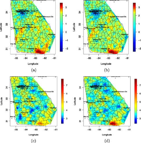
Figure 2: (a) Logtravel cost—1996; (b) Log travel cost—2008; (c) Log accessibility—1996; and (d) Log accessibility—2008.

In the following discussion, we contrast “horizontal equity” [Figure 2(a), (b)] measured using the travel cost without adjusting for the “utilization” of a service operation [in equation (1), $W(u,t)=1$ for any location $u$ and time point $t$] to “vertical equity” [Figure 2(c), (d)] which accounts for the expected utilization of a service.

Although difficult to assess visually, there are more extensive areas with lower (unadjusted) travel cost in 2008 than in 1996 in Georgia. On the other hand, the access to financial services is slightly lower in 2008 than in 1996 for highly populated regions, more specifically, Atlanta (see Supplemental Material 6 for the travel cost maps of metropolitan Atlanta). The primary reason for this contrast is that the increase in the number of new financial sites has a lower slope than the population growth in highly populated regions in Georgia. Consequently, these regions have weaker access compared to low density population areas, although the travel cost is small. These findings point to potential business opportunities for financial service providers.

This comparison between travel cost without and with utilization-adjustment motivates the need for correcting the travel cost for the expected utilization of a service. In our subsequent analysis, we will only focus on the utilization-adjusted travel cost.

4.2 Demographics data

In this study the demographic variables used to predict service accessibility include median household income, race and ethnicity data which are acquired from the Environmental Systems Research Institute (ESRI). The description of the methodology employed to obtain the demographic estimates at the census tract level is provided in Supplemental Material 5 of this paper. One has to bear in mind that the demographic estimates are measured with error which, in turn, will impact the estimates of the association between accessibility and the demographic variables.

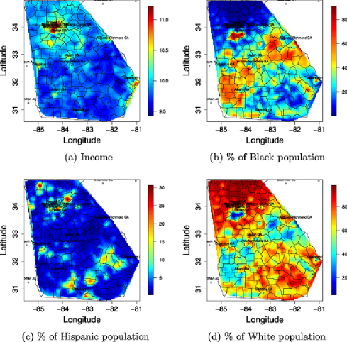
Figure 3: Demographic variables in Georgia.

Since the boundaries of census tracts are updated by the Census Bureau every ten years, our data set includes a change of boundaries. The Census Bureau provides the so-called “relationship files” to document the revisions of the 1990 to 2000 census tract boundaries. We map the data collected before 1999 to 2000 boundaries using the information in these relationship files.

Figure 3 shows the income level on the log scale and the percentages of Black, Hispanic and White populations for the last year of demographic data in this study. We do not show the plot of Asian percentages since overall in Georgia (except a small area in Atlanta) the percentage of Asian population is very low (close to zero). Contrasting the plots displaying the percentage of Black and White populations, we note that areas of high Black population have low White population and vice versa, pointing to significant segregation between black and white populations in Georgia. Indeed, the correlation is as high as $-0.98$, which suggests high collinearity between these two variables. At the same time, the collinearity between any other two demographic variables is low (see Table 1). Since there is high collinearity only between White and Black populations, we fit the varying coefficient models separately for $\{\mbox{income, Hispanic, White}\}$ and for $\{\mbox{income, Hispanic, Black}\}$.

Table 1: Correlation between demographic variables

Income	White	Black	Hispanic
1.00	$0.18$	$-0.27$	$0.37$
0.18	$1.00$	$-0.98$	$-0.01$
$-$0.27	$-0.98$	$1.00$	$-0.16$
0.37	$-0.01$	$-0.16$	$1.00$

4.3 Varying coefficient model: Motivation, results and findings

In this paper we introduce a framework for studying the equity of service accessibility for different groups of people identified by location or underlying socioeconomic variables. The data consist of a series of maps characterizing the access to financial services and a series of maps describing the demographic composition at the neighborhood level varying in time. The objective is to assess geographically-varying association patterns between accessibility and demographic variables over a period of several years.

Simple visual inspection of a large number of maps (13 for the accessibility measure and $13\times 4$ for four demographic variables) observed over a large geographic space goes beyond feasibility. Moreover, the existing models will only allow partial understanding of the dynamics in the equity of service accessibility. For example, space-varying coefficient models provide a one-year snapshot of the equity in service accessibility but will neither explain how it has changed over time nor account for the interaction between space and time associations. To model the space–time dynamics in the association between accessibility and socioeconomic variables jointly, we therefore apply the space–time varying coefficient model in Section 2.

In the application of the space–time varying coefficient model to the data in this study, we selected a small number of temporal basis functions ($M=7$) since we have a small number of time points; the space–time varying coefficients do not change significantly for various values of $M$. However, the estimated space–time varying coefficients vary with the number of spatial basis functions, $N$. For small $N$, the space-varying coefficients are smooth. Ruppert (2002) empirically suggests that after a minimum number of knots has been reached, the modeling bias is small. Therefore, we can control the modeling bias by using a large enough $N$; in our application $N$ can be as large as $S=1\mbox{,}624$. In contrast, the larger $N$ is, the more expensive the computation is. Consequently, we need to select $N$ for an optimal trade-off between modeling bias and computational feasibility. To select $N$, we used a residual-based analysis suggested by Wood (2006).

When interpreting the varying regression coefficients, one has to bear in mind that large values of the accessibility measure (population-adjusted travel cost) correspond to weak access to financial services. Moreover, significant association between accessibility and a demographic variable suggests that access to financial services is driven in part by the presence or the absence of the population group identified by the corresponding variable.

In this section we summarize our findings based on Figures 4, 5, 6 and 7, which include the following: [(3)]

The time-varying coefficients for income, % of Black population, % of Hispanic population and % of White population.

The space-varying association patterns for the four demographiccovariates in 2008 calculated from $\gamma(2008,s)=\alpha(2008)+\beta(s)+\break\operatorname{Interaction}(2008,s)$.

The point locations of inequities with respect to the four demographic covariates in 2008.

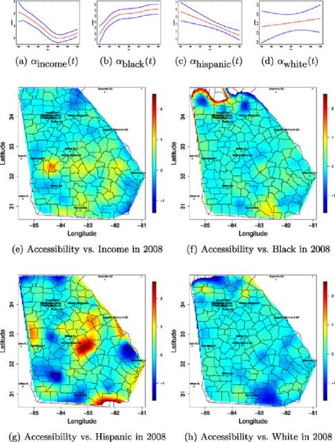
Figure 4: Georgia: The time-varying coefficients (a)–(d) and the spatial relationship pattern in 2008 for four demographic covariates—income, percentage of Black, Hispanic and White populations.

Figure 5: Georgia: Inequity locations in 2008 with respect to (wrt) four demographic covariates—income, percentage of Black, Hispanic and White populations.

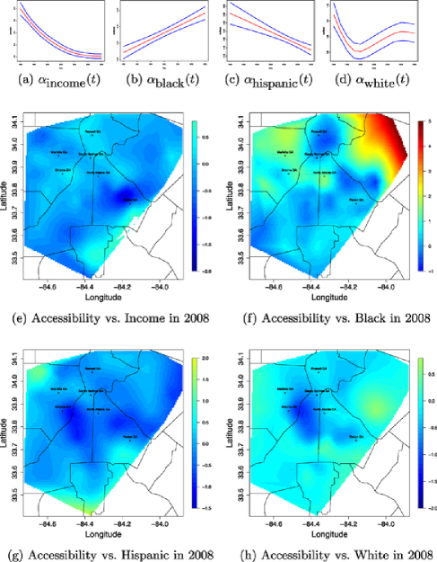
Figure 6: Atlanta: The time-varying coefficients (a)–(d) and the spatial relationship pattern in 2008 for four demographic covariates—income, percentage of Black, Hispanic and White populations.

Figure 7: Atlanta: Inequity locations in 2008 with respect to (wrt) four demographic covariates—income, percentage of Black, Hispanic and White populations.

The output figures summarize the space–time relationships between accessibility and the socioeconomic variables considered in this study. We highlight that without a rigorous modeling procedure, we cannot evaluate the significance of the associations to service accessibility. Therefore, using the space–time varying model is important not only for estimation of these associations but also for inference about their significance as described below.

We define locations of inequity with respect to income to be the spatial units $s$ such that $\gamma_{\mathrm{income}}(2008,s)$ is statistically significantly positive (positive correlation between income and utilization-adjusted travel cost). We also define locations of inequity with respect to race/ethnicity (percentage of Black, Hispanic and White populations) to be the spatial units $s$ such that $\gamma_{\mathrm{ethnicity}}(2008,s)$ is statistically significantly negative (negative correlation between percentage and utilization-adjusted travel cost). Statistical significance of the coefficients is derived from the simultaneous confidence bands of the spatial coefficients. Specifically, the coefficient at location $s$ is statistically significantly positive with 95% significance level if the lower bound of the confidence interval at $s$ is positive and it is statistically significantly negative if the upper bound of the confidence interval at $s$ is negative.

The time-varying coefficients corresponding to each demographic covariate and their confidence bands are in Figure 4(a)–(d) and Figure 6(a)–(d). Using the approach for evaluating the shape of the varying coefficients in Section 2.3, we infer that at the significance level of $95\%$, the time-varying coefficients for income are nonlinear, for the % of Black and Hispanic populations are linear whereas for the % of White population are constant. All space-varying coefficients are nonlinear.

Table 2: $P$-values for testing the significance of the space–time interaction in the varying coefficients for four demographic variables.

Covariate	Income	% of Black	% of Hispanic	% of White
$p$-value	$0.0018$	$0.0009$	$\approx$0	$\approx$0

We also evaluate the significance of the interaction terms for all four demographic variables. We apply the testing procedure for the space–time interaction term described in Section 2.3. The $p$-values are provided in Table 2. For all four demographic variables, the space–time interaction terms are highly significant, which implies that the space–time interactions in the association patterns are statistically significant; this suggests that the interaction term has a significant contribution to the spatial association patterns. Therefore, using a varying coefficient model with a space–time interaction term significantly contributes to a more accurate association analysis.

Time-varying association patterns. Following the inference procedure for shape evaluation, we infer that over the past 13 years in the state of Georgia, the association between the access to financial services and two demographic variables, income and the percentage of Hispanic population, has strengthened over time with a brief decrease in the last years, whereas the association between the access to financial services and the percentage of Black population has weakened. This suggests that access to financial services has become more and more dependent on the income level of the residents in a community and whether they are of Hispanic descent but less dependent on the race of the population.

Importantly, we cannot make inference about the magnitude of the association patterns since the constants for the temporal and spatial coefficients, $\tau_{0}$ and $\delta_{0}$, are nonidentifiable. For inference on the level and the direction (negative or positive) of the service accessibility association we need to investigate the space-varying association year by year as discussed below.

Space-varying association patterns. Controlling for race and ethnicity, the association between access to financial services and income level varies throughout the state of Georgia, with primarily weak positive association in the north but negative association in the south [Figure 4(e)]. This pattern is consistent with the income map in Figure 3(a); the income is consistently low in south and middle Georgia except for a few urban areas. This suggests that regions with low income population tend to also have lower access to financial services regardless of race and ethnicity. Moreover, there are only a few locations with statistically significant positive association between income and utilization-adjusted travel cost [Figure 5(a)]. This implies that although south Georgia consists primarily of low income population whereas north Georgia is more mixed with higher income population than south, financial services are present in both.

The map of the Black population percentage is not as uniform as its association to accessibility; there is a high density of the Black population in south Atlanta and in mid to south Georgia but not in the north [Figure 3(b)]. On the other hand, there are several locations with statistically significant inequities as shown in Figure 5(b), although the association of the % of Black population to financial service access is weak in Georgia except for the upper north. Most of these locations are in urban areas. We therefore conclude that the inequities in access to financial services with respect to the Black population are present but low throughout Georgia.

The association between travel cost and the % of Hispanic population is neither uniformly positive nor high [Figure 4(g)]. Areas of high Hispanic density population have low but statistically significantly positive association [Figure 5(c)]. This indicates that the presence of financial services decreases with the increase in Hispanic population.

In contrast, the association for White population is consistently weak throughout Georgia, although the White population density is high in most of Georgia except in the middle [Figure 3(d)]. Moreover, there are much fewer inequity locations than for Black and Hispanic populations and most are in rural areas [Figure 5(b)–(d)].

Since Atlanta is the largest city in Georgia with mixed income population and with a high percentage of Black, Hispanic and White populations, we applied the modeling procedures proposed in this paper to evaluate potential inequities in the Atlanta area and its surroundings.

The only time-varying coefficient that changes its shape in comparison to Georgia is for the White population; it has a nonlinear shape. There is an increase in the impact of the % of White population on the access to services (equivalently, a decrease in the impact on the travel cost) up to 2000 followed by a slower decrease thereafter.

Significant inequities in the Atlanta area are with respect to income and the Black population. The association of the % of Black population to service access is negative and strong in many communities in south and north Atlanta, implying significant inequities even after controlling for the income level. However, the association map does not fully overlap with the density of the Black population; that is, while South Atlanta has a large Black population [Figure 4(b), Supplemental Material 6], most inequities are in North Atlanta.

There is a positive association between income and access to financial services in south Atlanta, an area with a predominantly low income population [Figure 4(a), Supplemental Material 6]. Moreover, there is a weak association in north Atlanta and negative association in the east and west borders (possibly over-served areas). Therefore, when comparing the association map and its statistical significance to the map of the per capita income [Figure 4(a), Supplemental Material 6], we conclude that many communities with low and median income in central Atlanta have low access to financial services, as there is a statistically significant association between utilization-adjusted travel cost and income in these communities.

The association pattern for the % of Hispanic and % of White population is largely negative, with just a few communities with statistically significant positive association, although both population groups are well represented in Atlanta [Figure 4(c), (d), Supplemental Material 6], indicating insignificant inequities with respect to the Hispanic and White populations in Atlanta.

4.4 Multilevel varying coefficient model: Motivation, results and findings

Since monopoly is not common in service distribution, there is an intrinsic multilevel structure to service accessibility. At a higher level, we estimate the association to service accessibility over all service providers, whereas at a lower level, we estimate the deviations from the overall patterns associated with each service provider in the network. One simple approach would be to apply the space–time varying coefficient model to the accessibility measure computed for each service provider separately. However, this approach only takes into account the variability within the network of each service provider but not the variability between service providers; in other words, this simple approach does not allow estimating the deviations from the between-providers association patterns. The multilevel varying coefficient model in Section 3 estimates both overall space–time association patterns and the deviations from the overall pattern corresponding to each service provider.

In this section we discuss the association accessibility patterns to five financial service providers: Bank of America (BoA), Branch Banking and Trust Company (BB&T), Regions Bank, SunTrust Bank and Wachovia (Wells Fargo since 2008). In Supplemental Material 7 of this paper, we include the corresponding association patterns derived from the application of the multilevel space–time varying coefficient models.

All five banks are in the top 10 largest banks in the U.S., with a variety of financial services including retail and commercial banking, mortgages, insurance products, trust services and securities brokerage. SunTrust and Regions banks are mainly based in southern states, BB&T is a national bank, whereas BoA and Wachovia are national banks with international subsidiaries. Although Bank of America has dominated the financial service market for many years, due to mergers and acquisitions, SunTrust Bank and Wachovia (Wells Fargo since 2008) Bank now dominate the market. The only bank that has not increased the number of brunches in Georgia and, in fact, has closed some of them, is Bank of America.

Time-varying association patterns. Following the inference procedure for shape evaluation, we infer that the time-varying deviations from overall association patterns denoted in this paper by $\eta_{rp}(t_{i},s_{j})$, where $r$ is the index for the service provider and $p$ is the predictor index, are all approximately zero (not statistically significant) except for the deviation coefficients corresponding to income. Therefore, over the past 13 years in the state of Georgia, the association between the access to financial services and income is positive and has strengthened for BB&T and Bank of America beyond the global upward trend, indicating stronger association between service access and the income level in 2008 as compared to 1996. The income deviation coefficient for Wachovia is decreasing over time but negative, implying a decrease in association with respect to income. Finally, there are not significant systematic disparities in the provider-specific deviations from the overall association patterns for the ethnicity and race demographic variables.

Space-varying association patterns. The lowest association between service access and the four demographic variables is for Bank of America, Regions and Wachovia. The accessibility association patterns for these three banks do not deviate significantly from the global trends. The association of the percentage of Black and White populations to service accessibility is approximately zero, whereas the association to the percentage of Hispanic population is weak with mixed association throughout Georgia.

In urban and rural Georgia, the association between the access to BB&T services and the income level is highly positive, whereas the association for the % of Black and Hispanic populations is consistently weak and for the % of White population is approximately zero. Notably, the most significant inequities in 2008 for BB&T are with respect to income and they have increased over the 13 year period. For SunTrust, the service accessibility association to income is strong in south Georgia. There is weaker association in urban areas than in rural areas. Moreover, the association of the % of Black and Hispanic populations is weak.

The most significant inequities in Atlanta are with respect to income—high association between income and service accessibility for Bank of America and Regions in south Atlanta, for BB&T and SunTrust throughout Atlanta. There are contrasting association patterns for north and south Atlanta which also differ in their demographic decomposition. Generally, the accessibility association is low for the White population after controlling for income; this suggests equitable accessibility to financial services for the White population.

5 Final considerations

The methodological contributions described in this paper are twofold. First, we introduce a framework for the study of the equity of service accessibility across population groups with various demographic characteristics. This study allows characterization of the geographically varying equity patterns over a period of several years. Second, we investigate spatio-temporal estimation methods, which use the underlying structure of varying coefficient models. The first model estimates space–time varying association to a response variable (e.g., accessibility measure) of a series of predictors (e.g., demographic variables) jointly. The second model extends the first model to a response variable with a multilevel structure. Because of the complexity of the model parameters, we propose a simplified inference procedure based on confidence bands which allows evaluation of the shape of the varying coefficients.

We note that different service accessibility measures will provide different accessibility maps, and, therefore, different conclusions will be drawn for the study of service accessibility equity. In this paper, the underlying measure is defined as the utilization-adjusted travel cost; in Section 4.1 we compared the accessibility maps with and without correction for utilization and we concluded that the two measures will provide different perspectives in the equity of service accessibility, primarily for areas with low density population. A comparison study of accessibility measures is beyond the scope of this paper.

From the analysis of service accessibility using the space–time varying coefficient model, we identified significant but low inequities in some regions of Georgia with respect to income after controlling for race and ethnicity, and with respect to Black and Hispanic populations after controlling for income. These inequities have increased over time. The most predominant inequities in Atlanta are for Black population, although they have decreased over time. The association between income and service access is largely positive in Atlanta, suggesting potential inequities with respect to income as well. After accounting for service utilization, there are more significant inequities in urban areas than in rural areas; this may be due to the fact that the population in rural areas is more homogeneous.

In the analysis of service accessibility using the multilevel space–time model, we found for Georgia, and particularly for Atlanta, that the deviations from the between-provider association patterns are very insightful. Specifically, we learn, for example, that income-driven inequities for BB&T are significantly stronger when contrasted to the overall association to accessibility, whereas for other service providers, for example, Bank of America and Wachovia (Wells Fargo), there are not significant deviations from the between-providers association patterns.

Importantly, one challenge in space–time varying coefficient model estimation is whether an assumed pattern in a multiple predictor model can actually be recovered. For this, we conducted a simulation study with two predictors. The association patterns for both predictors are nonseparable in space and time, a more realistic simulation framework. For this simulation, the estimated coefficients are accurately estimated. We also evaluated the coverage and the power of the shape evaluation procedure discussed in Section 2.3. The power is lower for the time-varying components than for the space-varying ones; in this simulation study, the number of spatial points is $S=300$, whereas the number of time points is $T=15$, which may lead to lower accuracy in the shape evaluation of the varying coefficients. Moreover, the power depends on how smooth and close to the null hypothesis the shape function is.

We note that different service accessibility measures will provide different accessibility maps, and, therefore, different conclusions will be drawn for the study of service accessibility equity. In this paper the underlying measure is defined as the utilization-adjusted travel cost; in Section 4.1 we compared the accessibility maps with and without correction for utilization and we concluded that the two measures will provide different perspectives in the equity of service accessibility. A comparison study of various accessibility measures is beyond the scope of this paper.

One limitation of the study of service accessibility equity for large geographic regions (e.g., the US) using the space-varying coefficient models introduced in this paper is the computational aspect. Although we have reduced the estimation of multiple space–time varying coefficients with different smoothing levels to a simple mixed effects model, the estimation problem remains computationally intensive. A large geographic space requires a large number of knots, which in turn results in a model with a large number of random effects. In addition, because of the model decomposition into separable and nonseparable space–time coefficients, the number of variance components is large even for a small number of predictors (e.g., for three predictors in our study, we have a total of 12 variance components for the simple varying coefficient model but as many as 42 for the multilevel model). Ongoing research focuses on overcoming these challenges by using a backfitting estimation algorithm in the presence of multiple predictors.

References

- Assuncao (2003) {barticle}[auto:STB—2011-03-03—12:04:44] \bauthor\bsnmAssuncao, \bfnmR. M.\binitsR. M. (\byear2003). \btitleSpace varying coefficient models for small area data. \bjournalEnvironmetrics \bvolume14 \bpages453–473. \endbibitem
- Baladandayuthapani et al. (2008) {barticle}[mr] \bauthor\bsnmBaladandayuthapani, \bfnmVeerabhadran\binitsV., \bauthor\bsnmMallick, \bfnmBani K.\binitsB. K., \bauthor\bsnmHong, \bfnmMee Young\binitsM. Y., \bauthor\bsnmLupton, \bfnmJoanne R.\binitsJ. R., \bauthor\bsnmTurner, \bfnmNancy D.\binitsN. D. and \bauthor\bsnmCarroll, \bfnmRaymond J.\binitsR. J. (\byear2008). \btitleBayesian hierarchical spatially correlated functional data analysis with application to colon carcinogenesis. \bjournalBiometrics \bvolume64 \bpages64–73, 321–322. \biddoi=10.1111/j.1541-0420.2007.00846.x, issn=0006-341X, mr=2422820 \endbibitem
- Blackwell and Fox (2004) {bmisc}[auto:STB—2011-03-03—12:04:44] \bauthor\bsnmBlackwell, \bfnmA. G.\binitsA. G. and \bauthor\bsnmFox, \bfnmR. K.\binitsR. K. (\byear2004). \bhowpublishedRegional equity and smart growth: Opportunities for advancing social and economic justice in America. PolicyLink and Funders’ Network for Smart Growth and Livable Communities. PolicyLink, Oakland, CA. \endbibitem
- Crainiceanu, Staicu and Di (2009) {barticle}[pbm] \bauthor\bsnmCrainiceanu, \bfnmCiprian M.\binitsC. M., \bauthor\bsnmStaicu, \bfnmAna-Maria\binitsA.-M. and \bauthor\bsnmDi, \bfnmChong-Zhi\binitsC.-Z. (\byear2009). \btitleGeneralized multilevel functional regression. \bjournalJ. Amer. Statist. Assoc. \bvolume104 \bpages1550–1561. \biddoi=10.1198/jasa.2009.tm08564, issn=0162-1459, mid=NIHMS127980, pmcid=2897156, pmid=20625442 \endbibitem
- Crainiceanu et al. (2005) {barticle}[mr] \bauthor\bsnmCrainiceanu, \bfnmCiprian\binitsC., \bauthor\bsnmRuppert, \bfnmDavid\binitsD., \bauthor\bsnmClaeskens, \bfnmGerda\binitsG. and \bauthor\bsnmWand, \bfnmM. P.\binitsM. P. (\byear2005). \btitleExact likelihood ratio tests for penalised splines. \bjournalBiometrika \bvolume92 \bpages91–103. \biddoi=10.1093/biomet/92.1.91, issn=0006-3444, mr=2158612 \endbibitem
- Cressie (1993) {bbook}[mr] \bauthor\bsnmCressie, \bfnmNoel A. C.\binitsN. A. C. (\byear1993). \btitleStatistics for Spatial Data. \bpublisherWiley, \baddressNew York. \bidmr=1239641 \endbibitem
- Di et al. (2009) {barticle}[mr] \bauthor\bsnmDi, \bfnmChong-Zhi\binitsC.-Z., \bauthor\bsnmCrainiceanu, \bfnmCiprian M.\binitsC. M., \bauthor\bsnmCaffo, \bfnmBrian S.\binitsB. S. and \bauthor\bsnmPunjabi, \bfnmNaresh M.\binitsN. M. (\byear2009). \btitleMultilevel functional principal component analysis. \bjournalAnn. Appl. Statist. \bvolume3 \bpages458–488. \biddoi=10.1214/08-AOAS206, issn=1932-6157, mr=2668715 \endbibitem
- Diggle (1985) {barticle}[auto:STB—2011-03-03—12:04:44] \bauthor\bsnmDiggle, \bfnmP.\binitsP. (\byear1985). \btitleA kernel method for smoothing point process data. \bjournalJ. R. Stat. Soc. Ser. C Appl. Stat. \bvolume34 \bpages138–147. \endbibitem
- Fan and Zhang (2000) {barticle}[mr] \bauthor\bsnmFan, \bfnmJianqing\binitsJ. and \bauthor\bsnmZhang, \bfnmJin-Ting\binitsJ.-T. (\byear2000). \btitleTwo-step estimation of functional linear models with applications to longitudinal data. \bjournalJ. R. Stat. Soc. Ser. B Stat. Methodol. \bvolume62 \bpages303–322. \biddoi=10.1111/1467-9868.00233, issn=1369-7412, mr=1749541 \endbibitem
- Gelfand et al. (2003) {barticle}[mr] \bauthor\bsnmGelfand, \bfnmAlan E.\binitsA. E., \bauthor\bsnmKim, \bfnmHyon-Jung\binitsH.-J., \bauthor\bsnmSirmans, \bfnmC. F.\binitsC. F. and \bauthor\bsnmBanerjee, \bfnmSudipto\binitsS. (\byear2003). \btitleSpatial modeling with spatially varying coefficient processes. \bjournalJ. Amer. Statist. Assoc. \bvolume98 \bpages387–396. \biddoi=10.1198/016214503000170, issn=0162-1459, mr=1995715 \endbibitem
- Graves (2003) {barticle}[auto:STB—2011-03-03—12:04:44] \bauthor\bsnmGraves, \bfnmS. M.\binitsS. M. (\byear2003). \btitleLandscapes of predation, landscapes of neglect: A location analysis of payday lenders and banks. \bjournalThe Professional Geographer \bvolume55 \bpages303–317. \endbibitem
- Greven et al. (2008) {barticle}[mr] \bauthor\bsnmGreven, \bfnmSonja\binitsS., \bauthor\bsnmCrainiceanu, \bfnmCiprian M.\binitsC. M., \bauthor\bsnmKüchenhoff, \bfnmHelmut\binitsH. and \bauthor\bsnmPeters, \bfnmAnnette\binitsA. (\byear2008). \btitleRestricted likelihood ratio testing for zero variance components in linear mixed models. \bjournalJ. Comput. Graph. Statist. \bvolume17 \bpages870–891. \biddoi=10.1198/106186008X386599, issn=1061-8600, mr=2649072 \endbibitem
- Hastie and Tibshirani (1993) {barticle}[mr] \bauthor\bsnmHastie, \bfnmTrevor\binitsT. and \bauthor\bsnmTibshirani, \bfnmRobert\binitsR. (\byear1993). \btitleVarying-coefficient models. \bjournalJ. Roy. Statist. Soc. Ser. B \bvolume55 \bpages757–796. \bidissn=0035-9246, mr=1229881 \endbibitem
- Hoover et al. (1998) {barticle}[mr] \bauthor\bsnmHoover, \bfnmDonald R.\binitsD. R., \bauthor\bsnmRice, \bfnmJohn A.\binitsJ. A., \bauthor\bsnmWu, \bfnmColin O.\binitsC. O. and \bauthor\bsnmYang, \bfnmLi-Ping\binitsL.-P. (\byear1998). \btitleNonparametric smoothing estimates of time-varying coefficient models with longitudinal data. \bjournalBiometrika \bvolume85 \bpages809–822. \biddoi=10.1093/biomet/85.4.809, issn=0006-3444, mr=1666699 \endbibitem
- Huang, Wu and Zhou (2002) {barticle}[mr] \bauthor\bsnmHuang, \bfnmJianhua Z.\binitsJ. Z., \bauthor\bsnmWu, \bfnmColin O.\binitsC. O. and \bauthor\bsnmZhou, \bfnmLan\binitsL. (\byear2002). \btitleVarying-coefficient models and basis function approximations for the analysis of repeated measurements. \bjournalBiometrika \bvolume89 \bpages111–128. \biddoi=10.1093/biomet/89.1.111, issn=0006-3444, mr=1888349 \endbibitem
- Larson (2003) {barticle}[auto:STB—2011-03-03—12:04:44] \bauthor\bsnmLarson, \bfnmT.\binitsT. (\byear2003). \btitleWhy there will be no chain supermarkets in poor inner-city neighborhoods. \bjournalCalifornia Politics and Policy \bvolume7 \bpages22–45. \endbibitem
- Lehmann (1997) {bbook}[mr] \bauthor\bsnmLehmann, \bfnmE. L.\binitsE. L. (\byear1997). \btitleTesting Statistical Hypotheses, \bedition2nd ed. \bpublisherSpringer, \baddressNew York. \bidmr=1481711 \endbibitem
- Li and Ruppert (2008) {barticle}[mr] \bauthor\bsnmLi, \bfnmYingxing\binitsY. and \bauthor\bsnmRuppert, \bfnmDavid\binitsD. (\byear2008). \btitleOn the asymptotics of penalized splines. \bjournalBiometrika \bvolume95 \bpages415–436. \biddoi=10.1093/biomet/asn010, issn=0006-3444, mr=2521591 \endbibitem
- Liang, Wu and Carroll (2003) {barticle}[pbm] \bauthor\bsnmLiang, \bfnmHua\binitsH., \bauthor\bsnmWu, \bfnmHulin\binitsH. and \bauthor\bsnmCarroll, \bfnmRaymond J.\binitsR. J. (\byear2003). \btitleThe relationship between virologic and immunologic responses in AIDS clinical research using mixed-effects varying-coefficient models with measurement error. \bjournalBiostatistics \bvolume4 \bpages297–312. \biddoi=10.1093/biostatistics/4.2.297, issn=1465-4644, pii=4/2/297, pmid=12925523 \endbibitem
- Lovett et al. (2002) {barticle}[auto:STB—2011-03-03—12:04:44] \bauthor\bsnmLovett, \bfnmA.\binitsA., \bauthor\bsnmHaynes, \bfnmR.\binitsR., \bauthor\bsnmSunnenberg, \bfnmG.\binitsG. and \bauthor\bsnmGale, \bfnmS.\binitsS. (\byear2002). \btitleCar travel time and accessibility by bus to general practitioner services: A study using patient registers and GIS. \bjournalSoc. Sci. Med. \bvolume55 \bpages97–111. \endbibitem
- Marsh and Schilling (1994) {barticle}[auto:STB—2011-03-03—12:04:44] \bauthor\bsnmMarsh, \bfnmM. T.\binitsM. T. and \bauthor\bsnmSchilling, \bfnmD. A.\binitsD. A. (\byear1994). \btitleEquity measurement in facility location analysis—a review and framework. \bjournalEuropean J. Oper. Res. \bvolume74 \bpages1–17. \endbibitem
- Morris and Carroll (2006) {barticle}[mr] \bauthor\bsnmMorris, \bfnmJeffrey S.\binitsJ. S. and \bauthor\bsnmCarroll, \bfnmRaymond J.\binitsR. J. (\byear2006). \btitleWavelet-based functional mixed models. \bjournalJ. R. Stat. Soc. Ser. B Stat. Methodol. \bvolume68 \bpages179–199. \biddoi=10.1111/j.1467-9868.2006.00539.x, issn=1369-7412, mr=2188981 \endbibitem
- Morris et al. (2003) {barticle}[mr] \bauthor\bsnmMorris, \bfnmJeffrey S.\binitsJ. S., \bauthor\bsnmVannucci, \bfnmMarina\binitsM., \bauthor\bsnmBrown, \bfnmPhilip J.\binitsP. J. and \bauthor\bsnmCarroll, \bfnmRaymond J.\binitsR. J. (\byear2003). \btitleWavelet-based nonparametric modeling of hierarchical functions in colon carcinogenesis. \bjournalJ. Amer. Statist. Assoc. \bvolume98 \bpages573–597. \biddoi=10.1198/016214503000000422, issn=0162-1459, mr=2011673 \endbibitem
- Nychka and Saltzman (1998) {bmisc}[auto:STB—2011-03-03—12:04:44] \bauthor\bsnmNychka, \bfnmD.\binitsD. and \bauthor\bsnmSaltzman, \bfnmN.\binitsN. (\byear1998). \bhowpublishedDesign of air quality monitoring networks. Lecture Notes in Statist. 132 51–76. Springer, Berlin. \endbibitem
- Powell et al. (2007) {barticle}[auto:STB—2011-03-03—12:04:44] \bauthor\bsnmPowell, \bfnmL. M.\binitsL. M., \bauthor\bsnmSlater, \bfnmS.\binitsS., \bauthor\bsnmMirtcheva, \bfnmD.\binitsD., \bauthor\bsnmBao, \bfnmY. J.\binitsY. J. and \bauthor\bsnmChaloupka, \bfnmF. J.\binitsF. J. (\byear2007). \btitleFood store availability and neighborhood characteristics in the United States. \bjournalPreventive Medicine \bvolume44 \bpages189–195. \endbibitem
- Rice and Wu (2001) {barticle}[mr] \bauthor\bsnmRice, \bfnmJohn A.\binitsJ. A. and \bauthor\bsnmWu, \bfnmColin O.\binitsC. O. (\byear2001). \btitleNonparametric mixed effects models for unequally sampled noisy curves. \bjournalBiometrics \bvolume57 \bpages253–259. \biddoi=10.1111/j.0006-341X.2001.00253.x, issn=0006-341X, mr=1833314 \endbibitem
- Ruppert (2002) {barticle}[mr] \bauthor\bsnmRuppert, \bfnmDavid\binitsD. (\byear2002). \btitleSelecting the number of knots for penalized splines. \bjournalJ. Comput. Graph. Statist. \bvolume11 \bpages735–757. \biddoi=10.1198/106186002321018768, issn=1061-8600, mr=1944261 \endbibitem
- Ruppert, Wand and Carroll (2003) {bbook}[mr] \bauthor\bsnmRuppert, \bfnmDavid\binitsD., \bauthor\bsnmWand, \bfnmM. P.\binitsM. P. and \bauthor\bsnmCarroll, \bfnmR. J.\binitsR. J. (\byear2003). \btitleSemiparametric Regression. \bseriesCambridge Series in Statistical and Probabilistic Mathematics \bvolume12. \bpublisherCambridge Univ. Press, \baddressCambridge. \biddoi=10.1017/CBO9780511755453, mr=1998720 \endbibitem
- Serban (2011) {bmisc}[auto:STB—2011-03-03—12:04:44] \bauthor\bsnmSerban, \bfnmN.\binitsN. (\byear2011). \bhowpublishedSupplement to “A space–time varying coefficient model: The equity of service accessibility.” DOI:10.1214/11-AOAS473SUPP. \endbibitem
- Sim and Reid (1999) {barticle}[pbm] \bauthor\bsnmSim, \bfnmJ.\binitsJ. and \bauthor\bsnmReid, \bfnmN.\binitsN. (\byear1999). \btitleStatistical inference by confidence intervals: Issues of interpretation and utilization. \bjournalPhys. Ther. \bvolume79 \bpages186–195. \bidissn=0031-9023, pmid=10029058 \endbibitem
- Small and McDermott (2006) {bmisc}[auto:STB—2011-03-03—12:04:44] \bauthor\bsnmSmall, \bfnmM. L.\binitsM. L. and \bauthor\bsnmMcDermott, \bfnmM.\binitsM. (\byear2006). \bhowpublishedThe presence of organizational resources in poor urban neighborhoods: An analysis of average and contextual effects. Social Forces 84 1697. \endbibitem
- Staicu, Crainiceanu and Carroll (2010) {barticle}[pbm] \bauthor\bsnmStaicu, \bfnmAna-Maria\binitsA.-M., \bauthor\bsnmCrainiceanu, \bfnmCiprian M.\binitsC. M. and \bauthor\bsnmCarroll, \bfnmRaymond J.\binitsR. J. (\byear2010). \btitleFast methods for spatially correlated multilevel functional data. \bjournalBiostatistics \bvolume11 \bpages177–194. \biddoi=10.1093/biostatistics/kxp058, issn=1468-4357, pii=kxp058, pmcid=2830578, pmid=20089508 \endbibitem
- Talen (1997) {barticle}[auto:STB—2011-03-03—12:04:44] \bauthor\bsnmTalen, \bfnmE.\binitsE. (\byear1997). \btitleThe social equity of urban service distribution: An exploration of park access in Pueblo, Co and Macon, GA. \bjournalUrban Geography \bvolume18 \bpages521–541. \endbibitem
- Talen (2001) {barticle}[auto:STB—2011-03-03—12:04:44] \bauthor\bsnmTalen, \bfnmE.\binitsE. (\byear2001). \btitleSchool, community, and spatial equity: An empirical investigation of access to elementary schools in West Virginia. \bjournalAnnals of the Association of American Geographers \bvolume91 \bpages465–486. \endbibitem
- Talen and Anselin (1998) {bmisc}[auto:STB—2011-03-03—12:04:44] \bauthor\bsnmTalen, \bfnmE.\binitsE. and \bauthor\bsnmAnselin, \bfnmL.\binitsL. (\byear1998). \bhowpublishedAssessing spatial equity: An evaluation of measures of accessibility to public playgrounds. Environment and Planning A 30 595–613. \endbibitem
- Wahba (1990) {bbook}[mr] \bauthor\bsnmWahba, \bfnmGrace\binitsG. (\byear1990). \btitleSpline Models for Observational Data. \bseriesCBMS-NSF Regional Conference Series in Applied Mathematics \bvolume59. \bpublisherSIAM, \baddressPhiladelphia, PA. \bidmr=1045442 \endbibitem
- Waller et al. (2007) {barticle}[mr] \bauthor\bsnmWaller, \bfnmLance A.\binitsL. A., \bauthor\bsnmZhu, \bfnmLi\binitsL., \bauthor\bsnmGotway, \bfnmCarol A.\binitsC. A., \bauthor\bsnmGorman, \bfnmDennis M.\binitsD. M. and \bauthor\bsnmGruenewald, \bfnmPaul J.\binitsP. J. (\byear2007). \btitleQuantifying geographic variations in associations between alcohol distribution and violence: A comparison of geographically weighted regression and spatially varying coefficient models. \bjournalStoch. Environ. Res. Risk Assess. \bvolume21 \bpages573–588. \biddoi=10.1007/s00477-007-0139-9, issn=1436-3240, mr=2380676 \endbibitem
- Wood (2006) {bbook}[mr] \bauthor\bsnmWood, \bfnmSimon N.\binitsS. N. (\byear2006). \btitleGeneralized Additive Models: An Introduction with R. \bpublisherChapman & Hall/CRC, \baddressBoca Raton, FL. \bidmr=2206355 \endbibitem
- Wu and Liang (2004) {barticle}[auto:STB—2011-03-03—12:04:44] \bauthor\bsnmWu, \bfnmH.\binitsH. and \bauthor\bsnmLiang, \bfnmH.\binitsH. (\byear2004). \btitleBackfitting random varying-coefficient models with timedependent smoothing covariates. \bjournalScand. J. Statist. \bvolume31 \bpages3–20. \endbibitem
- Wu and Zhang (2002) {barticle}[mr] \bauthor\bsnmWu, \bfnmHulin\binitsH. and \bauthor\bsnmZhang, \bfnmJin-Ting\binitsJ.-T. (\byear2002). \btitleLocal polynomial mixed-effects models for longitudinal data. \bjournalJ. Amer. Statist. Assoc. \bvolume97 \bpages883–897. \biddoi=10.1198/016214502388618672, issn=0162-1459, mr=1941417 \endbibitem
- Zenk et al. (2005) {barticle}[pbm] \bauthor\bsnmZenk, \bfnmShannon N.\binitsS. N., \bauthor\bsnmSchulz, \bfnmAmy J.\binitsA. J., \bauthor\bsnmIsrael, \bfnmBarbara A.\binitsB. A., \bauthor\bsnmJames, \bfnmSherman A.\binitsS. A., \bauthor\bsnmBao, \bfnmShuming\binitsS. and \bauthor\bsnmWilson, \bfnmMark L.\binitsM. L. (\byear2005). \btitleNeighborhood racial composition, neighborhood poverty, and the spatial accessibility of supermarkets in metropolitan Detroit. \bjournalAm. J. Public Health \bvolume95 \bpages660–667. \biddoi=10.2105/AJPH.2004.042150, issn=0090-0036, pii=95/4/660, pmcid=1449238, pmid=15798127 \endbibitem
- Zhang (2004) {barticle}[mr] \bauthor\bsnmZhang, \bfnmDaowen\binitsD. (\byear2004). \btitleGeneralized linear mixed models with varying coefficients for longitudinal data. \bjournalBiometrics \bvolume60 \bpages8–15. \biddoi=10.1111/j.0006-341X.2004.00165.x, issn=0006-341X, mr=2043613 \endbibitem