Tentative Structural Features of a Gapped RVB State in the Anisotropic Triangular Lattice.

Abstract

The self-consistency equations for the independent order parameters as well as the free energy expression for the mean-field RVB model of the spin-1/2 Heisenberg Hamiltonian on the anisotropic triangular lattice is considered in the quasi-one-dimensional approximation. The solutions of the self-consistency equations in the zero-temperature limit are in fair agreement with the previous numerical analysis of the same model by other authors. In particular, the transition from the ungapped 1D-RVB state to the gapped 2D-RVB state occurs at an arbitrarily weak transversal exchange ($J_{2}\rightarrow 0)$ although the amount of the gap is exponentially small: $\frac{12J_{1}}{\pi}\exp\left(-\frac{2J_{1}}{J_{2}}\right)$, where $J_{1}$ is the longitudinal exchange parameter. The structural consequences of the formation of the 2D-RVB state are formulated by extending the famous bond order vs. bond length relation known for polyenes (one-dimensional Hubbard chains). Analytical estimates of this effect are given.

^aInstitut für anorganische Chemie, RWTH - Aachen University, Landoltweg 1, D-52056 Aachen, Germany;
^bPoncelet Lab., Independent University of Moscow, Moscow Center for Continuous Mathematical Education, Moscow, Russia;
^cDivision of Electrochemistry, Department of Chemistry, Moscow State University, Moscow, Russia.

1 Introduction

The RVB state originally proposed by Pauling [1] for describing the structure of the benzene molecule is being sought in many materials after Anderson’s [2] conjecture that it represents the ground state of cuprate-based high-temperature superconductors. The recently obtained [3] CuNCN phase whose structure is represented in Fig. 1 had been proposed as a candidate for an RVB ground state spin liquid [4] due to frustration of the effective exchange in the ab-plane where the 1/2 Cu²⁺ local spins form an anisotropic triangular lattice. The material had been subject of a series of measurements of its magnetic susceptibility, electric resistivity, heat capacity, also elastic neutron scattering as well as of ESR, NMR relaxation, and muon spin resonance (all vs. $T$) [3, 5, 6]. Although the neutron scattering (complete absence of the magnetic signal) as well as the susceptibility measurements (temperature independent paramagnetism above 80 K changed to approximately activation decay of the susceptibility below this temperature) strongly indicate the transition between the 1D-RVB regime at higher temperatures to the gapped 2D-RVB regime below 80 K the issue remains controversial [6] since the NMR and the $\mu$SR data so far better fit into a model of inhomogeneous spin-glass-like ground state.

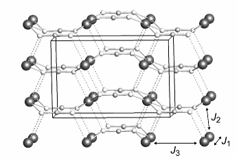
a

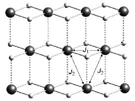
b

Figure 1: A look into the CuNCN crystal structure. A stronger $J_{1}$ extends in the $a$ direction; a somewhat weaker $J_{2}$ extends along the $b\pm a$ directions. The weakest $J_{3}$ extends in the $c$ direction and is not considered in the present paper.

In order to solve this dilemma we try to find out in the present paper what might be the structural concequences of the formation of two spin-liquid phases which is going to help in obtaining direct experimental evidence of this picture.

2 RVB mean-field analysis of an anisotropic triangular lattice system

2.1 Hamiltonian

A close inspection of the structure (Fig. 1) reveals that each Cu²⁺ ion can be effectively antiferromagnetically coupled to two of its neighbors forming a chain while somewhat weaker antiferromagnetic coupling with four more neighbors from two adjacent parallel chains results in a Heisenberg model on an anisotropic triangular lattice with the Hamiltonian:

$$\sum_{\mathbf{r}}\sum_{\mathbf{\tau}}J_{\mathbf{\boldsymbol{\tau}}}\mathbf{S}_{\mathbf{r}}\mathbf{S}_{\mathbf{r}+\tau}$$ (1)

where the coupling vectors $\mathbf{\tau}$ take three values $\tau_{i};\,i=1\div 3;\,\tau_{1}=(1,0);\,\tau_{2}=(\frac{1}{2},\frac{\sqrt{3}}{2});\,\tau_{3}=(\frac{1}{2},-\frac{\sqrt{3}}{2})$ with the interaction of the strength $J_{1}$ along the lattice vector $\mathbf{\mathbf{\tau}_{\mathrm{1}}}$ (two neighbors) and with a somewhat smaller strength $J_{2}$ along the lattice vectors $\mathbf{\mathbf{\tau}_{\mathrm{2}}}$ and $\mathbf{\mathbf{\tau}_{\mathrm{3}}}$ (two neighbors along each). This is precisely the setting for which Yunoki and Sorella [7] proposed that two (different) spin-singlet RVB (s-RVB) states are formed at different temperatures depending on the amount of anisotropy $\frac{J_{2}}{J_{1}}$ on the basis of their VMC calculations. Later Hayashi and Ogata [8] reproduced this result within a mean-field treatment which we basically follow here.

2.2 Equations of motion and self consistency equations

Hayashi and Ogata [8] base their analysis of the Hamiltonian eq. (1) on returning to the electron representation from the spin representation by the standard formulae:

$$\mathbf{S}_{i}=\frac{1}{2}c_{i\alpha}^{+}\mathbf{\boldsymbol{\sigma}}_{\alpha\beta}c_{i\beta},$$ (2)

where $c_{i\sigma}^{+}(c_{i\sigma})$ are the electron creation (annihilation) operators subject to the Fermi anticommutation relations; $\mathbf{\boldsymbol{\sigma}}_{\alpha\beta}$ are the elements of the Pauli matrices and the summation over repeating indices is assumed. For the latter one can derive equations of motion based on the Heisenberg representation in which each operator obeys the following equation of motion:

$$i\hbar\dot{A}=\left[A,H\right]$$ (3)

where $\left[,\right]$ stands for the commutator of the operators and the dot-on-top symbol for the time derivative. Applying this to the creation and annihilation operators $c_{\mathbf{r}\sigma}^{+}(c_{\mathbf{r}\sigma})$ and performing commutation, mean-field decoupling and Fourier transformation as done in [4, 8] results in mean-field equations of motion for these operators :

$$i\hbar\dot{c}_{\mathbf{k}\sigma}=-\frac{3}{2}\sum_{\mathbf{\tau}}J_{\mathbf{\boldsymbol{\tau}}}\xi_{\mathbf{\boldsymbol{\tau}}}\cos(\mathbf{k\tau})c_{\mathbf{k}\sigma} -\frac{3}{2}\sum_{\mathbf{\tau}}J_{\mathbf{\boldsymbol{\tau}}}\Delta_{\boldsymbol{\tau}} \cos(\mathbf{k\tau})c_{-\mathbf{k}-\sigma}^{+}$$

$$i\hbar\dot{c}_{\mathbf{k}\sigma}^{+}=\frac{3}{2}\sum_{\mathbf{\tau}}J_{\mathbf{\boldsymbol{\tau}}}\xi_{\mathbf{\boldsymbol{\tau}}}\cos(\mathbf{k\tau})c_{\mathbf{k}\beta}^{+} +\frac{3}{2}\sum_{\mathbf{\tau}}J_{\mathbf{\boldsymbol{\tau}}}\Delta_{\boldsymbol{\tau}}^{*} \cos(\mathbf{k\tau})c_{-\mathbf{k}-\sigma}$$ (4)

These reduce to the set of $2\times 2$ eigenvalue problems for each wave vector $\boldsymbol{\mathbf{k}}$:

$$\left(\begin{array}[]{cc}\xi_{\mathbf{k}}&\Delta_{\mathbf{k}}\\ \Delta_{\mathbf{k}}^{*}&-\xi_{\mathbf{k}}\end{array}\right)\left(\begin{array}[]{c}u_{\mathbf{k}}\\ v_{\mathbf{k}}\end{array}\right)=E_{\mathbf{k}}\left(\begin{array}[]{c}u_{\mathbf{k}}\\ v_{\mathbf{k}}\end{array}\right)$$ (5)

with

$$\xi_{\mathbf{k}} = -3\sum_{\mathbf{\tau}}J_{\mathbf{\boldsymbol{\tau}}}\xi_{\mathbf{\boldsymbol{\tau}}}\cos(\mathbf{k\tau})$$

$$\Delta_{\mathbf{k}} = 3\sum_{\mathbf{\tau}}J_{\mathbf{\boldsymbol{\tau}}}\Delta_{\mathbf{\boldsymbol{\tau}}}\cos(\mathbf{k\tau})$$ (6)

(summation over $\mathbf{\boldsymbol{\tau}}$ extends to $\pm\tau_{i};i=1\div 3$) which results in the eigenvalues (quasiparticle spectrum) of the form:

$$E_{\mathbf{k}} = \sqrt{\xi_{\mathbf{k}}^{2}+\left|\Delta_{\mathbf{k}}\right|^{2}}$$ (7)

whose eigenvectors are combinations of the destruction and creation operators with the above Bogoliubov transformation coefficients $u_{\mathbf{k}},v_{\mathbf{k}}$. These equations result in the self-consistency equations of the form:

$$\xi_{\mathbf{\boldsymbol{\tau}}} = -\frac{1}{2N}\sum_{\mathbf{k}}\exp(i\mathbf{k\tau})\frac{\xi_{\mathbf{k}}}{E_{\mathbf{k}}}\tanh\left(\frac{E_{\mathbf{k}}}{2\theta}\right)$$

$$\Delta_{\mathbf{\boldsymbol{\tau}}} = \frac{1}{2N}\sum_{\mathbf{k}}\exp(-i\mathbf{k\tau})\frac{\Delta_{\mathbf{k}}}{E_{\mathbf{k}}}\tanh\left(\frac{E_{\mathbf{k}}}{2\theta}\right)$$ (8)

for six order parameters $\xi_{\mathbf{\boldsymbol{\tau}}},\Delta_{\mathbf{\boldsymbol{\tau}}}$ defined as

$$\xi_{\mathbf{\boldsymbol{\tau}}} = \left\langle c_{\mathbf{r}+\boldsymbol{\tau}\sigma}^{+}c_{\mathbf{r}\sigma}\right\rangle$$

$$\Delta_{\boldsymbol{\tau}} = \left\langle c_{\mathbf{r}\alpha}c_{\mathbf{r}+\boldsymbol{\tau}\beta}\right\rangle.$$ (9)

It is remarkable and important for the subsequent treatment that the order parameters $\xi_{\mathbf{\boldsymbol{\tau}}}$ are in fact bond orders for the corresponding pairs of atoms.

2.3 Free energy

Following Ref. [9] one can write immediately the free energy in terms of the above order parameters:

$$F(\theta)=-\frac{\theta}{2N}\sum_{\mathbf{k}}\ln\left(2\cosh\left(\frac{E_{\mathbf{k}}}{2\theta}\right)\right)+\frac{3}{2}\sum_{\mathbf{\tau}}J_{\mathbf{\boldsymbol{\tau}}}\xi_{\mathbf{\boldsymbol{\tau}}}^{2}+\frac{3}{2}\sum_{\mathbf{\tau}}J_{\mathbf{\boldsymbol{\tau}}}\left|\Delta_{\mathbf{\mathbf{\boldsymbol{\tau}}}}\right|^{2}$$ (10)

where $\theta=k_{B}T$ and summation over $\mathbf{\boldsymbol{\tau}}$ extends to $\pm\tau_{i};i=1\div 3$. Minima of this expression with respect to $\xi_{\mathbf{\boldsymbol{\tau}}}$ and $\Delta_{\mathbf{\boldsymbol{\tau}}}$ correspond to various possible states of the system.

3 Simplified RVB on the anisotropic triangular lattice

The numerical analysis [8] shows that in agreement with general theorems [10] the order parameters satisfy additional phase relations

$$\arg\Delta_{\boldsymbol{\tau}_{2}}-\arg\Delta_{\boldsymbol{\tau}_{3}}=\pm\frac{\pi}{2}$$ (11)

which allows to reduce the number of order parameters to only two [11, 4]:

$$\sqrt{2}\xi=\xi_{\boldsymbol{\tau}_{1}};\sqrt{2}\eta=\left|\Delta_{\boldsymbol{\tau}_{2}}\right|=\left|\Delta_{\boldsymbol{\tau}_{3}}\right|$$ (12)

the first responsible for establishing the gapless 1D-RVB state within the chains and the second one for opening a gap and establishing the 2D-RVB in the transversal direction and other three order parameters set to be zero. It can be shown that this particular choice of the phases leads to the following form of the fermion quasiparticle spectrum:

$$E_{\mathbf{k}}^{2} = 18\left(J_{1}^{2}\xi^{2}\cos^{2}(\mathbf{k}_{x})+J_{2}^{2}\eta^{2}+J_{2}^{2}\eta^{2}\cos(\mathbf{k}_{x})\cos(\mathbf{k}_{y}\sqrt{3})\right).$$ (13)

This form of the quasiparticle spectrum allows for a simple analysis. Obviously in the 1D-RVB state ($\eta=0$) the spectrum has a vanishing dispersion in the $y$-direction:

$$E_{\mathbf{k}} =3\sqrt{2} \left|J\xi\cos(\mathbf{k}_{x}).\right|$$ (14)

It is gapless along the lines $\mathbf{k}_{x}=\pm\frac{\pi}{2}$ and contains ridges at $\mathbf{k}_{x}=0,\pm\pi$ extended in the $y$-direction. The corresponding density of the quasiparticle states (qDOS) is depicted in Fig. 2 (red). The divergence on the qDOS:

$$g(\varepsilon)=\frac{2}{\pi\sqrt{18J^{2}\xi^{2}-\varepsilon^{2}}}$$

on the upper border of the spectrum is obviously due to the abovementioned ridges in the spectrum of the quasiparticles. On the other hand the low-energy behavior of the system in the 1D-RVB state is controlled by a constant qDOS at the zero energy, which is perfectly reflected in the temperature independent paramagnetic susceptibility in the respective temperature region.

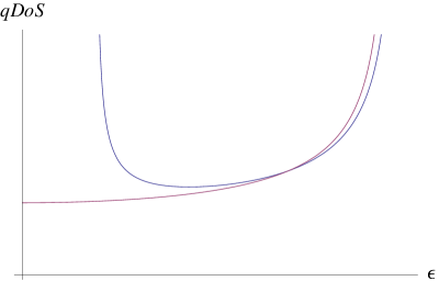
Figure 2: The schematic densities of the fermion quasiparticle states in the 1D-RVB (red) and 2D-RVB states (blue) of a system of 1/2 Heisenberg spins on the anisotropic triangular lattice. The 2D-RVB qDOS is built for the effective anisotropy parameter $a=\frac{1}{5}$ (see the text for details). In addition to the gap opening one may observe a slight shift of the energy at which the upper singularity occurs.

The transition to the 2D-RVB state is accompanied by a significant reorganization of the quasiparticle spectrum. Both the ridges at $\mathbf{k}_{x}=0,\pm\pi$ and the degeneration lines at $\mathbf{k}_{x}=\pm\frac{\pi}{2}$ disappear and are replaced by the critical points whose characteristics are given in Table 1. One can realize that in the 2D case the qDOS is mainly contributed by the logarithmic van Hove singularities due to the saddle points of the spectrum on top of the constant contributions coming from the minima and maxima of the quasiparticle spectrum. Physically it must be important that the values of the energy corresponding to the minima and maxima differ from the saddle point energies only in the second order in a small parameter of efficient anisotropy: $a=\frac{J_{2}\eta}{J_{1}\xi}$ so that one ultimately cannot expect anything, but some widening of the logarithmic peak of the qDOS on the upper bound of the spectrum. The most important changes occur at the lower bound of the spectrum, where a gap opens. As one can see from Table 1 the singular spectral weight must concentrate at the energy of the lower saddle points: $3\sqrt{2}J_{2}\eta$, although the lower boundary of the spectrum is smaller than this value in the fourth order with respect to efficient anisotropy.

Table 1: Critical points of the quasiparticle spectrum in the gapped spin liquid 2D-RVB state of a system of 1/2 Heisenberg spins on the anisotropic triangular lattice. $(\mathbf{k}_{x},\mathbf{k}_{y})$ stands for the coordinates of the critical point in the Brillouin zone, n is the degeneracy - total number of points of the given type; other entries are self-explanatory.

$(\mathbf{k}_{x},\mathbf{k}_{y})$	n	$E^{2}$	point type
$(0,\frac{\pi l}{\sqrt{3}});l=-2,0,2$	3	$18\left(J_{1}^{2}\xi^{2}+2J_{2}^{2}\eta^{2}\right)$	maximum
$(\pm\pi,\pm\frac{\pi}{\sqrt{3}})$	4	$18\left(J_{1}^{2}\xi^{2}+2J_{2}^{2}\eta^{2}\right)$	maximum
$(0,\pm\frac{\pi}{\sqrt{3}})$	2	$18J_{1}^{2}\xi^{2}$	saddle
$(\pm\pi,0)$	2	$18J_{1}^{2}\xi^{2}$	saddle
$(\pm\frac{\pi}{2},\pm\frac{\pi}{2\sqrt{3}})$	4	$18J_{2}^{2}\eta^{2}$	saddle
$(\pm\frac{\pi}{2},\pm\frac{\pi\sqrt{3}}{2})$	4	$18J_{2}^{2}\eta^{2}$	saddle
$(\pm\arccos\left(-\frac{J^{\prime 2}\eta^{2}}{2J^{2}\xi^{2}}\right),\pm\frac{2\pi}{\sqrt{3}})$	4	$18J_{2}^{2}\eta^{2}\left(1+\frac{3}{4}\frac{J_{2}^{2}\eta^{2}}{J_{1}^{2}\xi^{2}}\right)$	saddle
$(\pm\arccos\left(\frac{J^{\prime 2}\eta^{2}}{2J^{2}\xi^{2}}\right),\pm\frac{\pi}{\sqrt{3}})$	4	$18J_{2}^{2}\eta^{2}\left(1-\frac{1}{4}\frac{J_{2}^{2}\eta^{2}}{J_{1}^{2}\xi^{2}}\right)$	minimum
$(\pm\arccos\left(-\frac{J^{\prime 2}\eta^{2}}{2J^{2}\xi^{2}}\right),0)$	2	$18J_{2}^{2}\eta^{2}\left(1-\frac{1}{4}\frac{J_{2}^{2}\eta^{2}}{J_{1}^{2}\xi^{2}}\right)$	minimum

On the other hand we notice that the wave vectors of the critical points of the quasiparticle spectrum in the vicinity of its lower boundary either have the $\mathbf{k}_{x}$ component equal to $\pm\frac{\pi}{2}$ or differ from these values in a higher order of efficient anisotropy. Following [11] we notice that in this range of wave vectors the dispersion of quasiparticles in the $y$-direction is negligeably small. This brings us to the idea that one can hope that neglecting the $y$-dispersion when calculating the integral characteristics of the system does not affect the precision catastrophically. This may be considered as a quasi-one-dimensional approximation for the spectrum, which then takes the form:

$$E_{\mathbf{k}} = \sqrt{18\left(J_{1}^{2}\xi^{2}\cos^{2}(\mathbf{k}_{x})+J_{2}^{2}\eta^{2}\right)}.$$ (15)

Inserting this in the standard definition of the density of states we obtain as expected:

$$g(\varepsilon)=\frac{2\varepsilon}{\pi\sqrt{\left(18J_{1}^{2}\xi^{2}+18J_{2}^{2}\eta^{2}-\varepsilon^{2}\right)\left(\varepsilon^{2}-18J_{2}^{2}\eta^{2}\right)}}$$ (16)

which corresponds to the quasiparticle band ranging on the energy scale from $3\sqrt{2}J_{2}\eta$ to $3\sqrt{2}\sqrt{J_{1}^{2}\xi^{2}+J_{2}^{2}\eta^{2}}$ with its lower boundary being as explained above somewhat higher than the lower boundary of the exact spectrum and with the upper boundary being located between the upper boundary and logarithmic peak of the exact spectrum.

With use of the qDOS eq. (16) one can easily write the explicit expression for the free energy as relying on the general expression eq. (10). It reads as follows:

$$F=6J_{1}\xi^{2}+12J_{2}\eta^{2}-2\theta\intop g(\varepsilon)\ln\left(2\cosh\left(\frac{\varepsilon}{2\theta}\right)\right)d\varepsilon.$$ (17)

We do not expect that our results obtained in [4] with use of the high-temperature expansion:

$$\ln\left(2\cosh\left(\frac{E_{\mathbf{k}}}{2\theta}\right)\right)\approx\ln 2+\frac{1}{2}\left(\frac{E_{\mathbf{k}}}{2\theta}\right)^{2}-\frac{1}{12}\left(\frac{E_{\mathbf{k}}}{2\theta}\right)^{4}$$

which allowed to perform integration over the entire BZ without neglecting the $y$-dispersion are going to change. By contrast, in the low temperature regime we first rewrite

$$\theta\ln\left(2\cosh\left(\frac{\varepsilon}{2\theta}\right)\right)=\frac{\varepsilon}{2}+\theta\ln\left(1+\exp\left(-\frac{\varepsilon}{\theta}\right)\right)$$

and immediately obtain the ground state energy for the 2D-RVB state:

$$F(\theta=0)=6J_{1}\xi^{2}+12J_{2}\eta^{2}-\intop g(\varepsilon)\varepsilon d\varepsilon$$

The integral is done analytically [12]:

$$\frac{6\sqrt{2}}{\pi}\sqrt{J_{1}^{2}\xi^{2}+J_{2}^{2}\eta^{2}}\mathsf{E}\left(k\right)$$

where $\mathsf{E}(k)$ is the complete elliptic integral of the second kind of the modulus $k$ given by:

$$k^{2}=\frac{J_{1}^{2}\xi^{2}}{J_{1}^{2}\xi^{2}+J_{2}^{2}\eta^{2}}.$$

This result is not unexpected since it has a form characteristic for one-dimensional systems [13]. Taking derivatives with respect to the order parameters and setting them equal to zero results in self-consistency conditions:

$$1 = \frac{J_{1}}{\sqrt{2}\pi\sqrt{J_{1}^{2}\xi^{2}+J_{2}^{2}\eta^{2}}}\left(\mathsf{K}\left(k\right)-\mathsf{D}\left(k\right)\right)$$ (18)

$$1 = \frac{J_{2}}{2\sqrt{2}\pi\sqrt{J_{1}^{2}\xi^{2}+J_{2}^{2}\eta^{2}}}\mathsf{K}\left(k\right)$$

which are remarkably similar to the self-consistency conditions [14] in the one-dimensional Hubbard problem, the first being one for the bond order and the second being analogous to that for the gap or magnetization with the $J_{2}$ parameter taking part of the interaction parameter $U$ of the Hubbard model and $3\sqrt{2}J_{1}\xi$ being the effective one-dimensional bandwidth. In the 1D-RVB state the first of the conditions eq. (18) yields the amplitude of the order parameter $\xi$ reached at the zero temperature:

$$\xi_{0}=\frac{1}{\sqrt{2}\pi},$$ (19)

which is in perfect agreement with the numerical result of [8]. Inserting this in the second of the two conditions eq. (18), neglecting the terms with containing η as compared to those with ξ in the sums, and using the logarithmic asymptotic form of the complete elliptic integral of the first kind $\mathsf{K}$ we arrive to the self-consistent field-like estimate of the for $\eta$ and for the gap in the 2D-RVB state:

$$\eta = \frac{2\sqrt{2}}{\pi}\frac{J_{1}}{J_{2}}\exp\left(-\frac{2J_{1}}{J_{2}}\right)$$

$$3\sqrt{2}J_{2}\eta = \frac{12J_{1}}{\pi}\exp\left(-\frac{2J_{1}}{J_{2}}\right)$$

at zero temperatue. The latter result is in a fair agreement with the numerical study [11] where the pre-exponential factor in the gap was estimated to be 3.50 as compared to 12/π $\approx$ 3.82. Although the factor in the exponent was estimated to be 1.61 in [11] against our estimate of two, the general form of the dependence of the characteristics of the model on its parameters is reproduced. These results in agreement with the numerical results [11] and general behavior of one-dimensional models with interaction and show that at the zero temperature some nonvanishing value of the $\eta$ order parameter and the energy gap appear at arbitrarily weak interaction $J_{2}$ so that no critical point with respect to the anisotropy $J_{2}/J_{1}$ should be expected at zero temperature.

A further move consists in inserting the above expression for $\eta$ in the logarithm and retaining the terms proportional to $\Lambda k^{\prime 2};\Lambda=\ln\frac{4}{k^{\prime}};k\mathit{{}^{\prime}}^{2}=1-k^{2}$ in the equation for $\xi$ so that $\mathsf{K}\left(k\right)-\mathsf{D}\left(k\right)\approx 1-\Lambda k^{\prime 2}/2$. By doing so and retaining the terms up to second order in $\eta$ we obtain:

$$\xi=\frac{1}{\sqrt{2}\pi}-\frac{\sqrt{2}\pi J_{2}}{J_{1}}\eta^{2},$$ (20)

which represents the estimate of the bond order variation in the 2D-RVB state as compared to the 1D-RVB state.

This finding is in a fair and remarkable agreement with the numerical result of [11] where it was shown that in the region where the 2D-RVB state develops ($\eta\neq 0$) the $\xi$ parameter manifests a very weak depletion as compared to its 1D-RVB ($\eta=0$) value. Despite the fact that it must be not particularly strong this depletion can manifest itself in a geometry change, which in principle could be observed. The subsequent reasoning following the lines proposed in [15] shows how it can tentatively look like.

Assume that the lattice contribution to the total energy per copper site can be harmonically approximated as a function of the separation ρ between the Cu atoms in the a-direction (the shortest such separation in the structure): $K(\text{\leavevmode{r}}-\text{\leavevmode{r}}_{0})^{2}/2$, where $K$ is an effective elastic constant and $\text{\leavevmode{r}}_{0}$ is an equilibrium separation to be observed if the spin contribution eqs. (10),(17) to the energy are turned off. The spin contribution to the lowest order comes from the “kinetic energy” term and is given by $-(6\text{\textsurd}2)/\text{\leavevmode{p}}J_{1}\xi$. Assuming the dependence of the effective exchange integral on the interatomic separation in the form$J_{1}=J_{10}+J_{1}^{\prime}(\text{\leavevmode{r}}-\text{\leavevmode{r}}_{0})$ we easily arrive to the analog of the famous bond order vs. bond length relation [16] for the RVB states:

$$\text{\leavevmode{r}}-\text{\leavevmode{r}}_{0}=\frac{6\sqrt{2}}{\text{\leavevmode{p}}}(J_{1}^{\prime}\xi)/K,$$ (21)

where ρ is now the equilibrium interatomic separation in the presence of the spin contribution to the energy. Obviously, the separation is going to change according to the sign of the derivative of the effective exchange integral with respect to the interatomic separation increase ($J_{1}^{\prime}<0$). The latter condition is, however, natural, in the frame of the standard conception of the sources of the antiferromagnetic exchange. Indeed, these appear as a result of perturbative treatment of the one-electron hopping in a strongly interacting regime. Then one has: $J_{i}=(4t_{i}^{2})/U$ where $t_{i}$ is the intersite one-electron hopping parameter along the respective hopping vector $\boldsymbol{\tau}_{i}$ and $U$ is the on-site electron-electron repulsion parameter. Assuming a linear dependence of the hopping parameter on the interatomic separation: $t=t_{0}+t\mathit{{}^{\prime}}(\text{\leavevmode{r}}-\text{\leavevmode{r}}_{0})$ we arrive to an estimate $J_{1}^{\prime}=(8t_{0}t\mathit{{}^{\prime}})/U<0$ since one can easily see that the multipliers $t_{0}$ and $t\mathit{{}^{\prime}}$ must have opposite signs. Combining eqs. (20) and (21) we arrive to the estimate for the variation of the equilibrium interatomic separation in the 2D-RVB state:

$$\text{\leavevmode{d}\leavevmode{r}}=\text{\textendash}6J_{2}J_{1}^{\prime}\eta^{2}/J_{1}K$$

which immediately shows that the lattice parameter $a$ in CuNCN must manifest the same trend as the 2D-RVB gap ($J_{1}^{\prime}<0$), although with somewhat damped amplitude due to square in a small quantity $\eta$.

4 Conclusion

In the present paper we succeeded in obtaining analytical estimates for the parameters (order parameters, energy gap) of the 2D-RVB state and possible structural concequences of the variation of these parameters under a 1D to 2D-RVB transition conjectured recently [6] to be responsible for the observed temperature behavior of the magnetic susceptibility in CuNCN.

References

- [1] L. Pauling. J. Am. Chem. Soc. 48, 1132 (1926).
- [2] P. W. Anderson. Science 235 , 1196 (1987).
- [3] X.-H. Liu, R. Dronskowski, R. K. Kremer, M. Ahrens, C.-D. Lee, M.-H. Whangbo, J. Phys. Chem. C 112, 11013 (2008).
- [4] A. L. Tchougréeff, R. Dronskowski. arXiv:1008.0182v2.
- [5] H. Xiang, X. Liu, R. Dronskowski, J. Phys. Chem. C 113, 18891 (2009).
- [6] A. Zorko, P. Jeglič, A. Potočnik, D. Arčon, A. Balčytis, Z. Jagličič, X. Liu, A. L. Tchougréeff, R. Dronskowski, Phys. Rev. Lett. 107, 047208 (2011).
- [7] S. Yunoki, S. Sorella, Phys. Rev. B 74, 014408 (2006).
- [8] Y. Hayashi and M. Ogata. J. Phys. Conf. Ser. 150, 042053 (2009).
- [9] M. Ogata and H. Fukuyama. Rep. Progr. Phys. 71, 036501 (2008).
- [10] M. Ogata, J. Phys. Soc. Jpn. 72, 1839 (2003); F. C. Zhang, C. Gros, T. M. Rice and H. Shiba, Supercond. Sci. Technol. 1, 36 (1988).
- [11] Y. Hayashi, M. Ogata. arXiv:0704.1313v1; Y.Hayashi, M.Ogata, J. Phys. Soc. Jpn. 76, 053705 (2007).
- [12] Janke-Emde-Lösch. Tafeln Höhere Funktionen. 6. Auflage Neubearbeitet von F. Lösch. B. G. Teubner Verlagsgeselschaft, Stuttgart, 1960.
- [13] P. Fulde. Electron Correlations in Molecules and Solids. 2-nd edition. Springer-Verlag, Berlin et al., 1993.
- [14] A. E. Belinskii, A.L. Tchougréeff, I. A. Misurkin. Teor. i Eksp. Khim. 25, 513 (1989) [in Russian]; Theor. and Exp. Chem. 25, 475 (1989) [in English].
- [15] I. A. Misurkin, A. A. Ovchinnikov. J. Struct. Chem. 5, 888 (1965) [in Russian]; I. A. Misurkin, A. A. Ovchinnikov. Opt. Spectr. 16, 228 (1964) [in Russian]; I. A. Misurkin, A. A. Ovchinnikov, Usp. Khim. 46, 1833 (1977) [in Russian].
- [16] C. Coulson, A. Golebievski. Proc. Phys. Soc. 78, 1310 ( 1961).