Low-lying dipole response: isospin character and collectivity in ⁶⁸Ni, ¹³²Sn and ²⁰⁸Pb

Abstract

The isospin character, the collective or single-particle nature, and the sensitivity to the slope of the nuclear symmetry energy of the low-energy isovector dipole response (known as pygmy dipole resonance) are nowadays under debate. In the present work we study, within the fully self-consistent non-relativistic mean field (MF) approach based on Skyrme Hartree-Fock plus Random Phase Approximation (RPA), the measured even-even nuclei ⁶⁸Ni, ¹³²Sn and ²⁰⁸Pb. To analyze the model dependence in the predictions of the pygmy dipole strength, we employ three different Skyrme parameter sets. We find that both the isoscalar and the isovector dipole responses of all three nuclei show a low-energy peak that increases in magnitude, and is shifted to larger excitation energies, with increasing values of the slope of the symmetry energy at saturation. We highlight the fact that the collectivity associated with the RPA state(s) contributing to this peak is different in the isoscalar and isovector case, or in other words it depends on the external probe. While the response of these RPA states to an isovector operator does not show a clear collective nature, the response to an isoscalar operator is recognizably collective, for all analyzed nuclei and all studied interactions.

I Introduction

Collective phenomena in atomic nuclei have been in the past bort1998 ; hara2001 and constitute in the present paar2007 one of the most active and interesting topics of research in nuclear physics. Experimental data on giant resonances have allowed us to determine fundamental properties associated with the nuclear interaction in the nuclear medium, such as the nuclear incompressibility, the isoscalar effective mass at saturation, and the nuclear symmetry energy at some subsaturation density blai1995 ; agra2003 ; colo2004 ; rute2005 ; rein1999 ; trip2008 . With the advent of new experimental facilities employing rare isotope beams (RIBs) tanh1995 ; geis1995 ; muel2001 , the possibility of studying exotic modes in unstable nuclei is nowadays feasible. The low-energy peak present in the isovector dipole response of proton-deficient and neutron-rich nuclei, the so called Pygmy Dipole Resonance (PDR) klim2007 , has been experimentally investigated in several cases such as ^17-22O leis2001 , ^44,48Ca hart2000 ; hart2004 , ⁶⁸Ni weil2009 , ^{116-120,124,130,132}Sn adri2005 ; fult1969 and ²⁰⁸Pb ryez2002 . In addition, recent extensive theoretical calculations indicate that such a low-energy peak is a common property of neutron-rich nuclei tsun2011 . However, for this PDR, the isoscalar character, the collective or single particle nature and the sensitivity to the density dependence of the symmetry energy are nowadays under debate klim2007 ; tsun2011 ; carb2010 ; piek2011 ; rein2010 ; gamb2011 ; bara2011 ; yuks2011 Hereinafter, we will refer to the low-energy peak present in the isovector dipole response as pygmy dipole strength (PDS) instead of the commonly used PDR since the resonant (collective) nature of such a peak has not been confirmed yet.

Such an observable is not only important for nuclear structure applications. It also impacts on the determination of reaction rates in the astrophysical $r$-process paar2007 . While some theoretical investigations consider the PDS as a collective phenomena klim2007 ; tsun2011 ; carb2010 ; piek2011 , others ended up with opposite conclusions rein2010 . Within the formers, the PDS is basically understood as a resonant oscillation of the neutron skin against the isospin saturated proton-neutron core. In agreement with this picture, in Ref. carb2010 it has been found that a linear relation between the energy weighted sum rule (EWSR) exhausted by the PDS and the density dependence of the nuclear symmetry energy exists. The symmetry energy is a basic property of the nuclear equation of state that plays a crucial role in a variety of physical systems. From the very big: the size of a neutron star or its composition and structure latt2001 ; roca2008 ; to the very small: the neutron skin thickness of a heavy nucleus brow2000 ; cent2009 ; roca2011 . Within the latters, opposite to such a picture, the PDS has been postulated just as a shell effect dependent on the particular nucleus under study: in particular, the authors of Ref. rein2010 argue that the strong fragmentation shown by the strength function within their theoretical calculations is indicative of such a single particle shell effect rein2011 . As an example of the complexity of the problem, in Ref. gamb2011 the case of ⁴⁸Ca have been studied in detail. The authors concluded that only one of the low-lying excitations within the energy range 5-10 MeV can be described as a pygmy resonance. Finally, it is also important to mention that within some of the works in which the PDS is assumed to be collective, it has been stated that such a low-energy peak in the dipole response may, indeed, correspond to a toroidal mode vret2001 ; ryez2002 ; urba2011 or that it is weakly dependent on the isovector part of the nuclear effective interaction bara2011 .

For our study of the PDS on the measured even-even neutron-rich nuclei ⁶⁸Ni, ¹³²Sn and ²⁰⁸Pb that we take as representative of different mass regions, we adopt the fully self-consistent non-relativistic mean field (MF) approach based on Skyrme Hartree-Fock (HF) plus RPA. The MF approach provide a unique framework for the study of all nuclei along the periodic table except the lightest ones. Such models typically display a rather small root mean square (rms) deviation on binding energies when compared with a large set of experimental data paar2007 ; bend2003 ; vret2005 and are able, through the RPA approach, to predict the main features of Giant Resonances bort1998 ; hara2001 ; paar2007 . To assess the sensitivity of our analysis on the nuclear model, we employ three Skyrme parameter sets, namely SGII sgii , SLy5 sly5 and SkI3 ski3 . Since the low-energy isovector dipole response of neutron-rich nuclei may be related with the density derivative of the symmetry at saturation, the set of chosen models have been selected due to the wide range displayed for their predicted values of the $L$ parameter. Such a parameter is defined as $L\equiv 3\rho_{\infty}[\partial c_{\rm sym}(\rho)/\partial\rho]_{\rho_{\infty}}$ where $c_{\rm sym}(\rho)$ is the symmetry energy, $\rho$ is the nucleon density and $\rho_{\infty}$ is the nuclear saturation density. All the studied nuclei are spherical and double-magic. This renders our HF calculations relatively simple and the analysis clearer since neither pairing nor deformation should be included.

First and foremost, we are interested in the theoretical study of the main features displayed by the low-energy RPA state that give rise to the largest contribution to the PDS or, hereinafter, RPA-pygmy state. In our work, we shall investigate the isoscalar or isovector character displayed by the transition densities associated to the RPA-pygmy state, and the most relevant particle-hole ($ph$) excitations contributing to such a state. In particular, we will emphasize that different operators will produce a different number of coherent contributions from $ph$ amplitudes. This means that in the case of different experimental probes one will see the same RPA-pygmy state with a different associated degree of collectivity. In the final stage of the preparation of this manuscript we have become aware that a similar analysis has been performed in Ref. yuks2011 .

A brief summary of the employed formalism is given in Section II where some properties of the interactions we use are also detailed. In Section III, results are presented, analyzed and compared with available experimental data. Finally, our conclusions are laid in the last section.

II Formalism

In this section we present the general expression of the Skyrme interaction as well as some basic properties of the parametrizations used in our analysis. A brief description of the RPA formalism is also presented. We address the reader to Refs. sly5 ; vaut1972 ; bein1975 for further details on the Skyrme interaction.

II.1 Skyrme interaction

The Skyrme interaction is a zero-range, velocity-dependent interaction that describe nucleons with space, spin and isospin variables ${\bf r}_{i},\mbox{\boldmath$\sigma$}_{i}$ and $\mbox{\boldmath$\tau$}_{i}$. It is commonly written as in Ref. sly5 ,

$$V({\bf r}_{1},{\bf r}_{2}) = t_{0}(1+x_{0}P_{\sigma})\delta({\bf r})$$ (1)

$$+ \frac{1}{2}t_{1}(1+x_{1}P_{\sigma})[{\bf P}^{\prime 2}\delta({\bf r})+\delta({\bf r}){\bf P}^{2}]$$

$$+ t_{2}(1+x_{2}P_{\sigma}){\bf P}^{\prime}\cdot\delta({\bf r}){\bf P}$$

$$+ \frac{1}{6}t_{3}(1+x_{3}P_{\sigma})\rho^{\alpha}({\bf R})\delta({\bf r})$$

$$+ iW_{0}({\mbox{\boldmath$\sigma$}}_{1}+{\mbox{\boldmath$\sigma$}}_{2})\cdot[{\bf P}^{\prime}\times\delta({\bf r}){\bf P}]~{},$$

where ${\bf r}={\bf r}_{1}-{\bf r}_{2}$, ${\bf R}=\frac{1}{2}({\bf r}_{1}+{\bf r}_{2})$, ${\bf P}=\frac{1}{2i}({\bf\nabla}_{1}-{\bf\nabla}_{2})$, ${\bf P^{\prime}}$ is the hermitian conjugate of ${\bf P}$ (acting on the left), $P_{\sigma}=\frac{1}{2}(1+{\mbox{\boldmath$\sigma$}}_{1}\cdot{\mbox{\boldmath$\sigma$}}_{2})$ is the spin-exchange operator.

As mentioned already in the Introduction, we employ three Skyrme interactions: SGII sgii , SLy5 sly5 and SkI3 ski3 ; as many others, they have been accurately calibrated in order to reproduce some bulk properties (the binding energies and charge radii) of few selected stable nuclei, as well as some empirical nuclear matter properties such as the saturation energy and the saturation density (and others depending on the specific set). Throughout this work, we are mainly interested on the sensitivity of the PDS to the density derivative of the symmetry energy at saturation carb2010 . Since SGII, SLy5 and SkI3 are characterized by $L$ equal to, respectively, 37.63 MeV, 48.27 MeV and 100.52 MeV, they span a quite broad range (comparable with the one spanned by most of the modern and commonly used MF models available in the literature cent2009 ; roca2011 ).

II.2 Random Phase Approximation

The discrete RPA method is well-known from textbooks ring1980 ; rowe1980 . In our self-consistent approach, we build the residual interaction ($V_{\rm residual}^{qq^{\prime}}$) for the proton-proton ($qq^{\prime}$=$pp$), neutron-neutron ($qq^{\prime}$=$nn$) and proton-neutron ($qq^{\prime}$=$pn$) channels from the Skyrme-HF energy density functional, namely $V_{\rm residual}^{qq^{\prime}}\equiv\delta^{2}E_{\rm HF}/\delta\rho_{q}\delta\rho_{q^{\prime}}$. Then we solve fully self-consistently the RPA equations by means of the matrix formulation like in Refs. frac2005 ; tsil2006 . One should note that the continuum is discretized by setting the system in a large box.

For any operator $\hat{F}_{JM}$ the (reduced) transition strength or probability is given by

$$B(EJ,\tilde{0}\rightarrow\nu) = \left|\langle\nu||\hat{F}_{J}||\tilde{0}\rangle\right|^{2}$$ (2)

$$= \left|\sum_{ph}\left(X_{ph}^{(\nu)}+Y_{ph}^{(\nu)}\right)\langle p||\hat{F}_{J}||h\rangle\right|^{2},$$

where $\langle\nu||\hat{F}_{J}||\tilde{0}\rangle$ is the reduced matrix element of $\hat{F}_{JM}$ (see, e.g., Ref. bohr1969 ). The initial state in all studied nuclei, $|\tilde{0}\rangle$, correspond to the RPA ground-state with zero total angular momentum and $|\nu\rangle$ stands for a generic RPA excited state. The latter equation is also written in an alternative notation that will turn out to be useful for our present purposes. That is, each RPA transition $|\tilde{0}\rangle\rightarrow|\nu\rangle$ excited via $\hat{F}_{JM}$ is composed by all considered particle-hole ($ph$) pairs that couple to a total angular momentum $JM$. The relative contribution of each $ph$ excitation to the reduced matrix element $\langle\nu||\hat{F}_{J}||\tilde{0}\rangle$ is accounted by the $X_{ph}^{(\nu)}$ and $Y_{ph}^{(\nu)}$ RPA amplitudes that specify a given eigenvector of the RPA secular matrix ring1980 . For the analysis of the single particle or collective character of a given excitation in the response function, it is convenient to write the reduced amplitude as follows:

$$A_{ph}(EJ,\tilde{0}\rightarrow\nu)=\left(X_{ph}^{(\nu)}+Y_{ph}^{(\nu)}\right)\langle p||\hat{F}_{J}||h\rangle.$$ (3)

This is because Eq. (3) allows one to determine the coherency (relative sign) and magnitude ($|A_{ph}(EJ,\tilde{0}\rightarrow\nu)|$) of all the $ph$ contributions to the reduced transition probability. An RPA state is claimed to be a resonant excitation if the corresponding reduced amplitude is composed by several $ph$ excitations similar in magnitude and adding coherently.

The strength function is defined as usual,

$$S(E)=\sum_{\nu}|\langle\nu||\hat{F}_{J}||\tilde{0}\rangle|^{2}\delta(E-E_{\nu}),$$ (4)

where $E_{\nu}$ is the eigenenergy associated to the RPA state $|\nu\rangle$. Its moments can be calculated as

$$m_{k}=\int dE\ E^{k}S(E)=\sum_{\nu}|\langle\nu||\hat{F}_{J}||\tilde{0}\rangle|^{2}E_{\nu}^{k}.$$ (5)

Another quantity of interest that characterizes the relationship of each excited state with the ground state, is the transition density. Its integral with a multipole operator gives the corresponding transition amplitude of that operator. With the help of the $X^{(\nu)}$ and $Y^{(\nu)}$ amplitudes of a given RPA state $|\nu\rangle$, one can construct the radial part of its transition density defined by $\delta\rho_{\nu}({\bf r})\equiv\langle\nu|\hat{\rho}({\bf r})|\tilde{0}\rangle=\delta\rho_{\nu}(r)Y^{*}_{JM}(\hat{r})$ as follows,

$$\delta\rho_{\nu}(r) = \frac{1}{\sqrt{2J+1}}\sum_{ph}\left(X_{ph}^{(\nu)}+Y_{ph}^{(\nu)}\right)$$ (6)

$$\times\langle p||Y_{J}||h\rangle\frac{u_{p}(r)u_{h}(r)}{r^{2}}~{},$$

where $u_{\alpha}(r)$ is the solution to the Skyrme-HF radial equations corresponding to the single particle state $\alpha$. Note that the summations in the expression above can be done for neutrons or protons separately. This allows one to calculate the neutron and proton transition densities $\delta\rho_{\nu_{q}}(r)$ ($q=n,p$) and define accordingly the isoscalar (IS) and isovector (IV) transition densities as

$$\delta\rho_{\nu}^{\rm(IS)}(r) \equiv \delta\rho_{\nu_{n}}(r)+\delta\rho_{\nu_{p}}(r)\quad{\rm and}$$ (7)

$$\delta\rho_{\nu}^{\rm(IV)}(r) \equiv \delta\rho_{\nu_{n}}(r)-\delta\rho_{\nu_{p}}(r).$$ (8)

The interest of the transition densities relies on the fact that their spatial shape reveal the nature of the excitations: volume or surface type, isoscalar or isovector, etc. Moreover, they can be used as input in calculations of inelastic scattering cross sections. More details of our implementation of RPA can be found in Ref. colo2011 .

As our theoretical study will be devoted to the low energy dipole response in even-even neutron-rich nuclei, we define the isoscalar (IS) and isovector (IV) dipole operators ($J=1$) used for the different calculations:

$$\hat{F}_{1M}^{\rm(IS)}=\sum_{i=1}^{A}r^{3}_{i}Y_{1M}(\hat{r}_{i}),$$ (9)

$$\hat{F}_{1M}^{\rm(IV)}=\sum_{i=1}^{A}r_{i}Y_{1M}(\hat{r}_{i})\tau_{z}(i).$$ (10)

Note that the lowest order term in the IS dipole operator coming from the expansion of the Bessel functions ($r$) does not reproduce a physical excitation but a translation of the whole system. This is the reason why the IS dipole operator in Eq. (9) is proportional to the following term ($r^{3}$) in such an expansion.

The translational mode should in principle be decoupled from the physical excitations within the RPA. However, as in any numerical implementation, the decoupling is not perfect. Therefore, part of this state, known as the spurious state, overlaps with the physical RPA states. There are different ways to correct this overlap ring1980 ; kazu2011 . Our prescription is detailed in Appendix A, where we show how one can subtract the spurious state from the neutron and proton transition densities. The reliability of our method can be seen in Fig. 1 where we compare the strength function —calculated by convoluting the corresponding reduced transition probability of (Eq. 2) with a Lorenzian of 1 MeV width— for the isoscalar dipole response predicted by the SLy5 interaction sly5 for a test nucleus (²⁰⁸Pb) in three cases: in one case the spurious state has not been subtracted (solid curve), in the second case the spurious state has been subtracted by correcting the isoscalar dipole operator Eq. (9) with the addition of a term $-\eta r_{i}Y_{1M}(\hat{r}_{i})$ where $\eta=5\langle r^{2}\rangle/3$ like in Ref. giai1981 (dashed line), and finally in the last case the spurious state has been subtracted as explained in Appendix A (dot-dashed line).

From this figure one clearly sees that the different prescriptions for correcting the spurious state are completely equivalent. The advantage of our method relies on the fact that, by construction, we exactly subtract the spurious state from the neutron and proton transition densities, and these are among the quantities that we discuss in detail below.

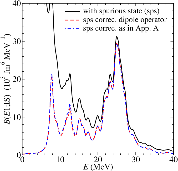
Figure 1: (Color online) Strength function in the case of the SLy5 interaction sly5 for a test nucleus (²⁰⁸Pb) as a function of the excitation energy for three cases: (i) the spurious state has not been subtracted (solid line), (ii) the spurious state has been subtracted by correcting the isoscalar dipole operator Eq. (9) (dashed line), and (iii) the spurious state has been subtracted as explained in the Appendix A (dot-dashed line).

In the case of the IV dipole operator, we have to subtract the dipole motion associated with the displacement of the neutron and proton center-of-mass. It can be done by modifying the operator (10) as follows,

$$\hat{F}_{1M}^{\rm(IV)}=\frac{Z}{A}\sum_{n=1}^{N}r_{n}Y_{1M}(\hat{r}_{n})-\frac{N}{A}\sum_{p=1}^{Z}r_{p}Y_{1M}(\hat{r}_{p}).$$ (11)

Last but not least, calculations beyond RPA may of course to some extent change the quantitative picture. It is known that correlations associated with coupling with 2 particle- 2 hole (2p-2h) configurations, or particle-phonon configurations, tend to shift the strength downward and increase its fragmentation. However, at least in the cases that have been studied in Refs. sarchi ; litvinova , these changes do not destroy the qualitative features associated with the PDS, namely the isospin character, the overall behavior of the transition densities and the collective or single-particle character of the states. We leave aside in our study the debated case of Ca isotopes discussed in Refs. gamb2011 ; tert2007 ; papa2011 .

III Results

In this Section we present a detailed study of the dipole response of ⁶⁸Ni, ¹³²Sn and ²⁰⁸Pb as predicted by the Skyrme interactions SGII, SLy5 and SkI3 within the formalism described in Section II. The results are organized as follows. We present for each nucleus the isoscalar and isovector dipole strength functions.

In order to have a simple estimate for the collectivity displayed by the different dipole responses, we plot also the reduced transition probabilities in single particle units (s.p.u., or Weisskopf units bohr1969 ). Such unit is based on a macroscopic approach. One evaluates the average transition rate of a typical excitation in terms of the angular momentum carried by the probe, and the mass radius of the nucleus under analysis; in this way, the result is nucleus-independent. By following Ref. bohr1969 , one can calculate the isovector dipole response in Weisskopf units accounting for the center of mass correction as,

$$B_{\rm W}^{\rm(IV)}(E1)=\frac{3^{3}R^{2}}{4^{3}\pi}\times\left\{\begin{array}[]{rl}~{}\left(\frac{N}{A}\right)^{2}&{\rm for~{}protons}\\ &\\ \left(-\frac{Z}{A}\right)^{2}&{\rm for~{}neutrons}\end{array}\right.$$ (12)

where the radius $R$ is taken to be $r_{0}A^{1/3}$ and $r_{0}$ is the radius of the average sphere that one nucleon occupies, at the standard saturation density of 0.16 fm^-3 (that is, $r_{0}=1.14$ fm). For the isoscalar dipole case, once the spurious state has been subtracted as explained in the previous section, one finds

$$B_{\rm W}^{\rm(IV)}(E1)=\frac{3}{4\pi}\left(\frac{1}{2}R^{3}-\eta\frac{3}{4}R\right)^{2}=\frac{3R^{6}}{4^{3}\pi}$$ (13)

with $\eta=\frac{5}{3}\langle r^{2}\rangle$ and $\langle r^{2}\rangle=\frac{3}{5}R^{2}$. The sum over all nucleons in Eqs. (12) and (13) coincides in good approximation (around 10%$-$20%) with the corresponding total RPA strength, although there exist some mass dependence: heavier nuclei are better reproduced by the estimate provided by the Weisskopf units. Such a unit allows us to account qualitatively for the nature of different excitations since a given RPA state will contribute with several single particle units if it is collective. Moreover, it also enables the comparison between the results obtained for different nuclei.

Then, we focus on the low-energy region in order to investigate the RPA-pygmy state leading to the PDS. We show, first, the neutron and proton transition densities associated with such a state for each interaction and nucleus. The analysis of the transition densities may be very illustrative since they allow one to distinguish some spatial details related to the dynamics of every excitation. For example, one could understand if either nucleons from the surface or from the interior of the nucleus are contributing more to the excitation, and this is crucial to estimate which reaction is more efficient in exciting this mode. Besides this, the comparison between the neutron and proton transition densities informs us about the relative motion of neutrons with respect to protons, or in other words, on the isoscalar or isovector character of each RPA state.

For this aim, we also use a local criterion to study quantitatively the isoscalar and isovector splitting of the RPA-pygmy state paar2009 based on the following. At each radial distance $r_{i}$, where $i=1\ldots N$ at which the neutron and proton transition densities are calculated, we define that a certain RPA state is 70% isoscalar if at least the 70% of the calculated points fulfill the condition $|\delta\rho_{\nu}^{\rm(IS)}(r)|>|\delta\rho_{\nu}^{\rm(IV)}(r)|$. Moreover, we will exploit the possibility of analyzing the isoscalar or isovector nature of the RPA-pygmy state in different regions of the nucleus. Specifically, we impose the above defined criteria of isoscalarity in two additional regions: one in the internal part of the nucleus, i.e. from 0 fm to R/2 and the other in external part of the nucleus, namely from R/2 to R.

Finally, we analyze the most relevant particle-hole ($ph$) excitations contributing to the RPA-pygmy state. To this end, we calculate the magnitude and sign (coherency) with which each $ph$ excitation contribute to the isovector (IV) and isoscalar (IS) dipole reduced transition probability ($B(E1;\xi)$ where $\xi=$IV or IS). For that, we have used the isoscalar $A_{ph}^{q}(E1;\xi=IS)$ and isovector $A_{ph}^{q}(E1;\xi=IV)$ reduced amplitudes defined in Eq. (3).

III.1 Strength functions in ⁶⁸Ni, ¹³²Sn and ²⁰⁸Pb

In this subsection we analyze the main features displayed by the strength function Eq. (4) associated to the isovector and isoscalar dipole response of ⁶⁸Ni, ¹³²Sn and ²⁰⁸Pb. It has been calculated by convoluting the corresponding reduced transition probability, Eq. (2), with a Lorenzian of 1 MeV width. The low-energy dipole response of all studied nuclei has been measured ryez2002 ; adri2005 ; weil2009 .

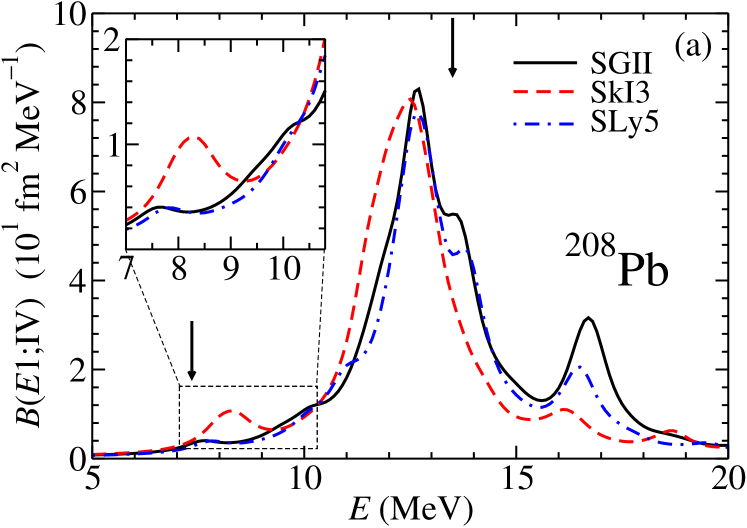
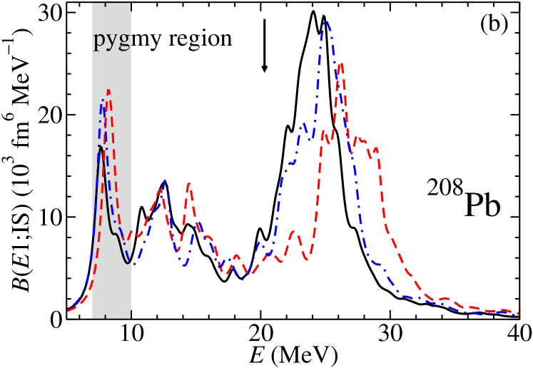
Figure 2: (Color online) Strength function corresponding to the isovector (a) and isoscalar (b) dipole response of ²⁰⁸Pb as a function of the excitation energy. The inset in (a) displays in a larger scale the pygmy region. In both figures the predictions of SGII, SLy5 and SkI3 are depicted. Black arrows indicate the experimental centroid energies for the PDS ($E=7.37$ MeV within a window of $6-8$ MeV) ryez2002 , for the ISGDR ($E=20.3\pm 2$ MeV garg1999 ) and the energy peak for the IVGDR ($E=13.43$ MeV and a total width of $2.42$ MeV berm1975 ).

Table 1: Excitation energy $E$ and isoscalar ($\xi=IS$) and isovector ($\xi=IV$) reduced transition probabilities $B(E1;\xi)$ corresponding to the RPA-pygmy states of ⁶⁸Ni, ¹³²Sn and ²⁰⁸Pb as predicted by SGII, SLy5 and SkI3 interactions.

	force	$E$	$B(E1;IS)$	$B(E1;IV)$
		[MeV]	[fm6]	[fm2]
68Ni	SGII	9.77	1.9$\times 10^{3}$	1.4
	SLy5	9.30	1.7$\times 10^{3}$	0.8
	SkI3	10.45	3.0$\times 10^{3}$	3.6
132Sn	SGII	8.52	3.3$\times 10^{3}$	1.2
	SLy5	8.64	1.0$\times 10^{4}$	1.6
	SkI3	9.23	1.1$\times 10^{4}$	7.4
208Pb	SGII	7.61	1.7$\times 10^{4}$	2.9
	SLy5	7.74	2.8$\times 10^{4}$	2.8
	SkI3	8.01	1.9$\times 10^{4}$	6.6

We start analyzing the results for ²⁰⁸Pb. In Fig. 2a we show the strength function corresponding to the isovector dipole response as a function of the excitation energy. The inset displays in a larger scale the pygmy region. In Fig. 2b, the same quantities are shown but this time for the isoscalar dipole response as a function of the excitation energy. In both figures, the predictions of the three selected interactions are shown. The centroid energies of the PDS and the Isoscalar Giant Dipole Resonance (ISGDR) as well as the energy peak in the Isovector Giant Dipole Resonance (IVGDR) for ²⁰⁸Pb as predicted by the employed interactions ($E=7.6-8.0$ MeV, $E=20-21$ MeV and $E=12-13$ MeV, respectively) fairly agree with the experimental data ($E=7.37$ MeV within a window of $6-8$ MeV ryez2002 , $E=20.1-20.5$ MeV garg1999 and $E=13.43$ MeV and a total width of $2.42$ MeV berm1975 , respectively). Consequently, the RPA predictions of SGII, SLy5 and SkI3 may allow us to elucidate the microscopical structure and properties of the PDS. In Table 1 the excitation energy and isoscalar and isovector reduced transition probabilities of the RPA-pygmy state —i.e. the RPA state which give rise to the largest peak in the PDS region— are detailed for all the sudied nuclei as predicted by SGII, SLy5 and SkI3. In the case of ²⁰⁸Pb we find an excitation energy of $E=7.61$ MeV for SGII, $E=7.74$ MeV for SLy5 and $E=8.01$ MeV for SkI3. We qualitatively observe that the low-energy peak found in the IV and IS dipole responses of ²⁰⁸Pb shows an increasing and outward trend with the excitation energy as the value of the parameter $L$ increases. This behavior is in agreement with Ref. carb2010 where the energy weighted sum rule or $m_{1}$ for the PDS was found to be linearly correlated with $L$ in mean-field models.

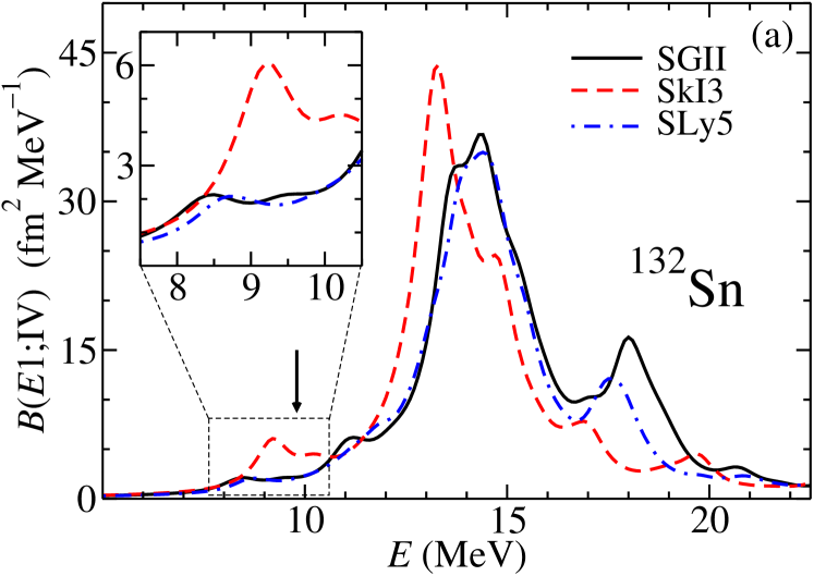
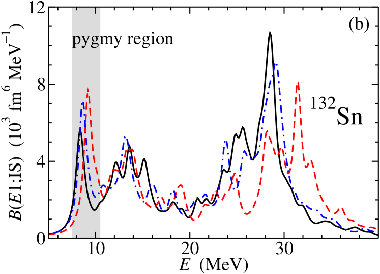
Figure 3: (Color online) Same as Fig. 2 for ¹³²Sn. The experimental value for the peak energy of the PDS ($E=9.8\pm 0.7$ MeV) is indicated by a black arrow adri2005 .

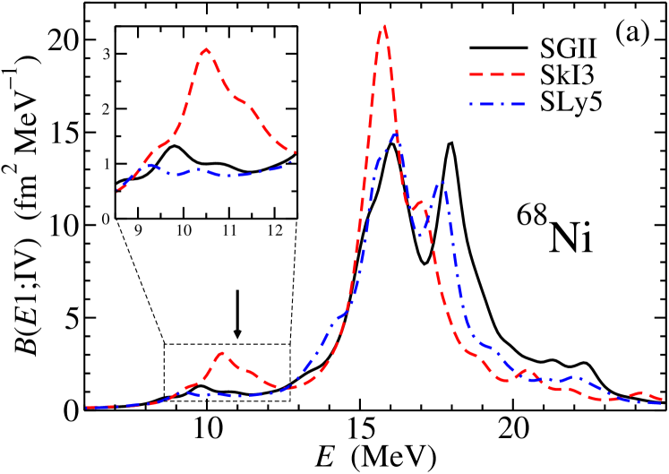
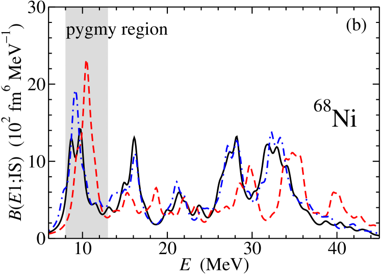
Figure 4: (Color online) Same as Fig. 2 for ⁶⁸Ni. The experimental value for the peak energy of the PDS ($E=11$ MeV and an energy width estimated to be less than 1 MeV) is indicated by a black arrow weil2009 .

In the case of ¹³²Sn and ⁶⁸Ni, the strength functions for the dipole response are depicted in Figs. 3a and 4a (IV) and Figs. 3b and 4b (IS), respectively. Again, the predictions of SGII, SLy5 and SkI3 ($E=8.5-9.2$ MeV for ¹³²Sn and $E=9.3-10.4$ MeV for ⁶⁸Ni) are in rather good agreement with the measured data ($E=9.1-10.5$ MeV for ¹³²Sn adri2005 and $E=11$ MeV and an energy width estimated to be less than 1 MeV for ⁶⁸Ni weil2009 ). In the case of ¹³²Sn, the RPA-pygmy state predicted by SGII correspond to a state with an excitation energy of $E=8.52$ MeV while SLy5 predicts $E=8.64$ MeV and SkI3 $E=9.23$ MeV. And for ⁶⁸Ni, the values predicted by SGII, SLy5 and SkI3 for the excitation energy of the RPA-pygmy state are respectively: $E=9.77$ MeV, $E=9.30$ MeV and $E=10.45$ MeV. Qualitatively in both nuclei, it seems again that the larger the value of $L$, the higher the values predicted for the excitation energy and the larger the different peaks arising in the low-energy region (see Figs. 3 and 4). In addition, we observe for all nuclei that the PDS is an order of magnitude smaller than the IVGDR and that its isoscalar counterpart is of the same order of magnitude than the corresponding ISGDR.

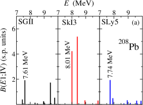
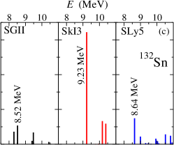
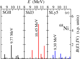
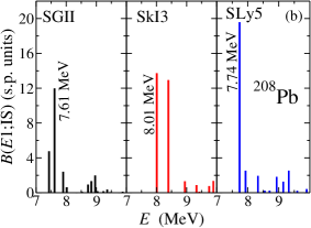
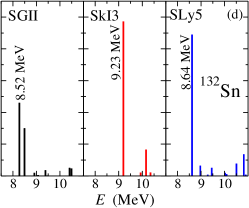
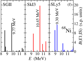
Figure 5: (Color online) Reduced transition probabilities for the isovector dipole response [(a), (c) and (e)] and isoscalar dipole response [(b), (d) and (f)], in the case of ²⁰⁸Pb [(a) and (b)], ¹³²Sn [(c) and (d)] and ⁶⁸Ni [(e) and (f)] in s.p. units, as a function of the excitation energy and as predicted by the selected MF interactions. Note that we only show the energy region relevant for our study of the RPA-pygmy state.

III.2 Reduced transition probability in single particle units as an indicator of collectivity

In Fig. 5, we focus on the relevant region for the study of PDS and show the reduced transition probabilities in single particle units [see Eqs. (12) and (13) and the related discussion]. The excitation energies of the RPA-pygmy state are also depicted. We display again both the isovector (Figs. 5a, 5c and 5e) and isoscalar (Figs. 5b, 5d and 5f) dipole responses.

Firstly, we focus on the isovector dipole response of ²⁰⁸Pb (see Fig. 5a). Our calculations predict an RPA-pygmy state characterized by $\approx$ 2-4 single particle units: this result does not pin down clearly the nature of the state. As a reference, the RPA state leading to the largest values of the reduced transition strength in the IVGDR contribute with about 30 single particle units if the strength is fragmented, and with more than 60 if the strength is concentrated in one single peak. This is a clear indication of the collective nature of the IVGDR. From Fig. 5b, where the isoscalar or compression dipole response of the same nucleus is depicted for the used Skyrme interactions, the RPA state leading to the pygmy peak is contributing with 15-20 single particle units, very similarly in magnitude to those displayed by the largest peak in the same isoscalar response at larger excitation energies and that can be seen in Fig. 2b. These large values indicate the collective character of the RPA-pygmy state when it is excited by an isoscalar probe.

In Figs. 5c and 5e (IV) and Figs. 5d and 5f (IS), the reduced transition probabilities in single particle units for the case of ¹³²Sn and ⁶⁸Ni are depicted, respectively. Note that we show only the low energy region. As mentioned, the single particle units normalize the absolute value of $B(E1;\xi)$ for all nuclei. This statement is qualitatively fullfiled by all the interactions: $B(E1,IV)$ corresponding to the RPA-pygmy state in ⁶⁸Ni, ¹³²Sn and ²⁰⁸Pb as calculated with SGII lead to 1.9, 1.1 and 1.9 s.p. units, respectively. For the case of SLy5, we find 1.1, 1.5 and 1.9 s.p. units, respectively. And, finally, for the case of SkI3, we find 4.9, 6.4 and 4.2 s.p. units, respectively. For the isoscalar response, the $B(E1,IS)$ of the same excited states in ⁶⁸Ni, ¹³²Sn and ²⁰⁸Pb as calculated with SGII lead to 12, 9 and 12 s.p. units, respectively. For the case of SLy5, we find 11, 18 and 19 s.p. units, respectively. And, finally, for the case of SkI3, we find 20, 19 and 14 s.p. units, respectively.

Despite the fact that the reduced transition probabilities in s.p. units can be only used as a qualitative estimator of the collectivity displayed by a given RPA excitation, we can conclude that while the isoscalar dipole response of all studied nuclei and within all employed interactions seems to indicate that the RPA-pygmy state develope a certain amount of collectivity, the isovector response of the same excited state does not provide a clear trend: the collectivity displayed is very weak and depends on the used model.

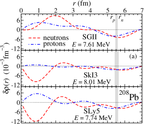
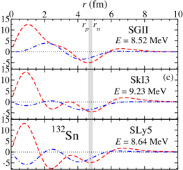
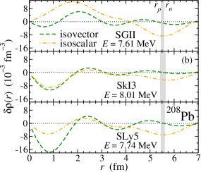
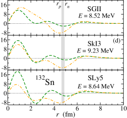
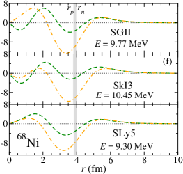
Figure 6: (Color online) Neutron and proton [(a), (c) and (e)] and isoscalar and isovector [(b), (d) and (f)] transition densities of the RPA-pygmy state, as a function of the radial distance, for ²⁰⁸Pb [(a) and (b)], ¹³²Sn [(c) and (d)] and ⁶⁸Ni [(e) and (f)]. The predictions of SGII, SLy5 and SkI3 are shown. Proton ($r_{p}$) and neutron ($r_{n}$) rms radii are indicated for each interaction by the edges of the grey region.

III.3 The low-energy RPA states: isoscalar or isovector character?

A collective excited state can be said to be purely isovector if the transition densities of protons and neutrons scale as Z and N, respectively, and have opposite phase. On the other side, a collective excited state can be defined as purely isoscalar if the neutron and proton transition densities scale in absolute value in the same way, but have the same sign. These two cases are extreme. As isospin is not a good quantum number in finite nuclei, and is more and more broken as the neutron excess increases, the most common situation corresponds to a mixture of a certain degree of isoscalarity and isovectoriality, that can be better seen by looking at the neutron and proton transition densities.

The isoscalar or isovector nature of the low-energy RPA states has been already studied in Ref. paar2009 in the case of ¹⁴⁰Ce. In this work, it was found that the low-lying dipole states of ¹⁴⁰Ce are split into two groups depending on their isospin structure. More recently, similar conclusions were found in a study of the pygmy dipole strength in ¹²⁴Sn endr2010 , where it has been stated that the theoretical calculations were dominated by a low-lying isoscalar component basically due to oscillations of the neutron skin thickness of the nucleus under study. It is important to note that both investigations were reported to be in qualitative agreement with the available experimental data.

On the basis of the above mentioned works and the definitions given in Eqs. (8) and in the text around, we present a more systematic study of the isospin structure of the low-energy RPA states as predicted by the forces SGII, SLy5 and SkI3 for the studied ⁶⁸Ni, ¹³²Sn and ²⁰⁸Pb nuclei. First of all, we plot the neutron and proton, as well as the isoscalar and isovector transition densities corresponding to the RPA-pygmy state as predicted by each interaction in order to illustrate how these low-energy transition densities behave.

We show the neutron and proton transition densities in Figs. 6a, 6c and 6e, and the isoscalar and isovector transition densities in Figs. 6b, 6d and 6f, respectively. All of them, correspond to the RPA-pygmy state. The position of the proton ($r_{p}$) and neutron ($r_{n}$) rms radii corresponds to the edges of the grey region that defines in this way the neutron skin thickness predicted by each interaction.

For the case of ²⁰⁸Pb, it can be seen from Fig. 2a that neutrons and protons oscillate differently depending on the interaction but in all cases the surface has a dominant isoscalar character. On the contrary, the interior or bulk region is not dominated by the isoscalar or isovector component but it is a mixture of them. The isoscalar or isovector dominance is better seen in Fig. 6b. At the surface of the nucleus the isovector transition density of the RPA-pygmy state is very close to zero, while the isoscalar one is not.

In Figs. 6c (protons and neutrons) and 6d (IS and IV), we display the transition densities for the case of ¹³²Sn. It is interesting to note that the situation is very similar to the one found in ²⁰⁸Pb.

The neutron and proton transition densities corresponding to the RPA-pygmy state in ⁶⁸Ni are depicted in Fig. 6e, and the corresponding isoscalar and isovector ones are displayed in Fig. 6f. The behavior of the different transition densities is predicted to be very similar within the studied models. This did not hold for ¹³²Sn and ²⁰⁸Pb where some qualitative differences arose. Therefore, it is even more clear in this case that the interior of ⁶⁸Ni is not dominated by isoscalar or isovector components. At the surface of the nucleus, the isoscalar part dominates but the isovector part is not very small as it happened for ¹³²Sn or ²⁰⁸Pb.

Then, we apply our criteria for defining a 70% isoscalar RPA state [see text after Eq. (8)] to all calculated excited states and plot their contribution to the isovector dipole strength function. We calculate the same quantity for different regions. First, we apply the criteria to those states that are 70% isoscalar in the region between 0 and $R$, where $R=r_{0}A^{1/3}$ (left panels in Fig. 7), then to those which are 70% isoscalar in the internal part of the nucleus, namely between 0 and $R/2$ (central panels in the same figure), and finally to those which are 70% isoscalar in the external part of the nucleus between $R/2$ and $R$ (right panels of the same figure). Specifically, in Fig. 7a, we show the above mentioned calculations for ²⁰⁸Pb as predicted by SLy5 (dashed line). As a guidance, we also show the total isovector dipole stregth function (solid line). The results predicted by the other interactions in the case of ²⁰⁸Pb are very similar and we are not showing them. From such a figure, it is evident that the RPA states which are mostly isoscalar in the whole region [0,R] (left panel in Fig. 7a) and in the external part of the nucleus [R/2,R] (right panel in Fig. 7a) are essentially the same ones since both give rise to almost the same contributions: most of the PDS and a small contribution to the rest of the strength function. In the central panel, where we represent those RPA states that are 70% isoscalar in the internal region of the nucleus [0,R/2], we confirm that there is no essential contribution from them to the state giving rise to the PDS.

In Figs. 7b and 7c, we show the same quantities but for ¹³²Sn as predicted by SGII and for ⁶⁸Ni as predicted by SkI3, respectively. Qualitatively, the same results found for ²⁰⁸Pb are now found in these figures. Again, we do not show the results for the other studied interactions since they are very similar and the same conclusions can be drawn.

Our results indicate that one is allowed to qualitatively distinguish the PDS from the IVGDR, and state that while the latter strength is basically isovector and involves the motion of mainly internal nucleons, the former is more isoscalar than isovector and involves the motion of external nucleons, that are mainly neutrons in a neutron rich nucleus.

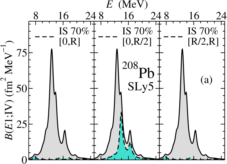
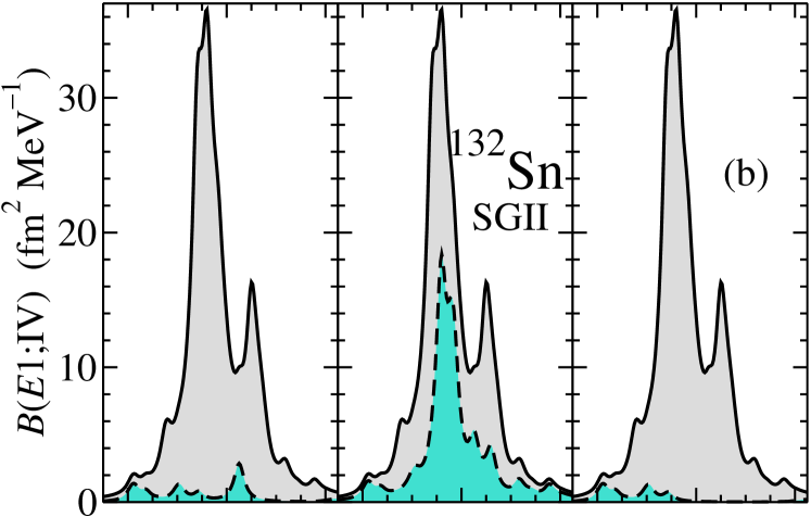
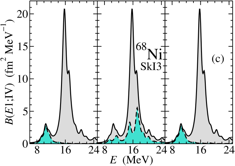
Figure 7: (Color online) Strength function corresponding to the isovector dipole response of ²⁰⁸Pb (a), ¹³²Sn (b) and ⁶⁸Ni (c) as a function of the excitation energy (solid lines), and partial contribution due to those states which are at least 70% isoscalar (dashed line): for each of the panels, the RPA states that are at least 70% isoscalar between 0 and $R$ are considered in the panel at the left hand side, those which have this feature between 0 and $R/2$ are considered in the central panel, and those which are like that between $R/$2 and $R$ are considered in the panel at the right hand side. See text for further explanations.

III.4 The most relevant particle-hole excitations in the low-energy region

The RPA states are build as a superposition of particle-hole ($ph$) excitations. A given RPA state shows a collective character under the action of an external operator if there are many $ph$ excitations providing non negligible contributions (each associated with a transition amplitude and the sum of $X_{ph}^{(\nu)}$ and $Y_{ph}^{(\nu)}$) that add coherently in Eq. (2). Therefore, within our approach, the collective nature of a peak in the response function of a nucleus is always hidden in the RPA states.

For these reasons, our purpose in this subsection is to analyze the contributions of the different $ph$ excitations to the RPA-pygmy states depending on the operator used to excite the nucleus. In particular, we study the isoscalar and isovector dipole responses of the RPA-pygmy states since we are most interested in them. Such a study will allow us to quantify the collectivity displayed by each RPA state depending on the operator, nucleus and interaction used for the theoretical calculations, and detect if there are common trends in the microscopic structure.

First of all, we show in Fig. 8a the neutron (black) and proton (red) single-particle MF levels close to the Fermi energy for ²⁰⁸Pb as predicted by SGII (left panel), SLy5 (right panel) and SkI3 (middle panel). The proton levels show a rather similar ordering and spacing for all the interactions. On the contrary, the neutron levels differ more when different interactions are compared.

In Figs. 8b and 8c, also for the case of ²⁰⁸Pb, we show all the neutron (black) and proton (red) $ph$ contributions to the reduced amplitude $A_{ph}^{q}(E1;\xi)$ [see Eq. (3)] as a function of their excitation energy for the isovector and isoscalar dipole responses, respectively. Both reduced amplitudes have been calculated for the case of the RPA-pygmy state predicted by the different MF models. Notice that not all contributions can be seen from these figures since most of them are very small.

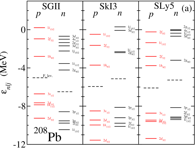
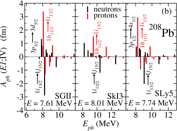
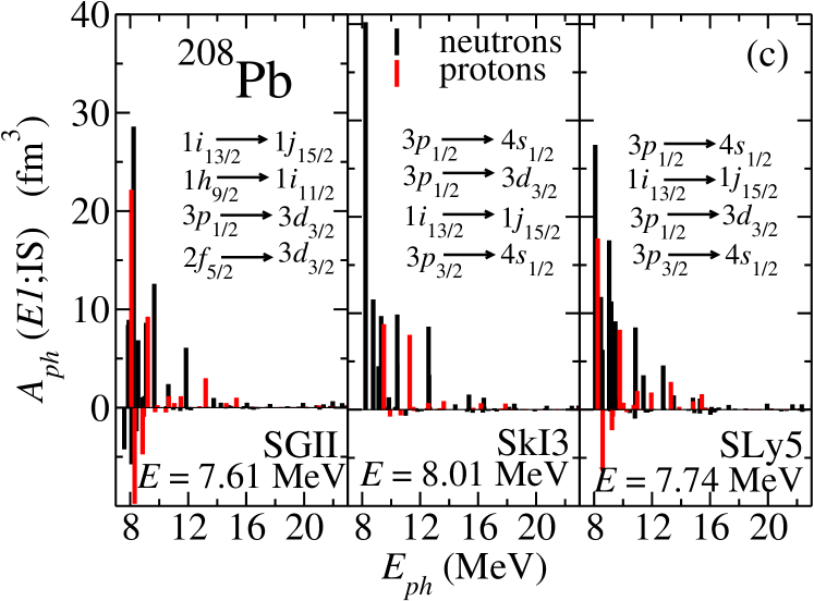
Figure 8: (Color online) Proton and neutron single particle levels of ²⁰⁸Pb as predicted by the different MF models (a). The Fermi level is indicated by a dashed black line. All $ph$ contributions to the isovector reduced amplitude corresponding to the ²⁰⁸Pb RPA-pygmy state as a function of the $ph$ excitation energy (c). All studied models are shown. Largest neutron $ph$ contributions are also listed in decreasing order from top to bottom. Same as (b) but for the isoscalar reduced amplitude (c).

It is evident from Fig. 8b that the contributions of the most relevant $ph$ excitations to the isovector reduced amplitude are only a few in number and there is some amount of destructive interference. Accordingly, we have seen that their total contribution to the isovector reduced transition strength in s.p. units do not clearly exceed one. Opposite to that, it is also evident from Fig. 8c that the contributions of the most relevant $ph$ excitations to the isoscalar reduced transition amplitude are basically coming from neutron transitions, and that most of them add coherently. This is, actually, one of the basic features to assert that a given RPA state is collective.

In Table 2 in Appendix B, we show the numerical details of the ten neutron and proton $ph$ excitations providing the largest contributions to the isovector and isoscalar $A_{ph}^{q}(E1;\xi)$. We also indicate in the figures and table the involved single particle orbitals corresponding to the largest contributions to the reduced amplitudes. In particular, we generally find within all the employed models that the dynamics of the low-energy isoscalar dipole response of ²⁰⁸Pb seems to be governed by the excitations of the outermost neutrons, namely those that form the neutron skin thickness of this nucleus. From the analysis of the $ph$ contributions, we conclude that while the low-energy isoscalar dipole response of ²⁰⁸Pb arising form the RPA-pygmy state can be considered as a collective mode in all studied models, the PDS can not.

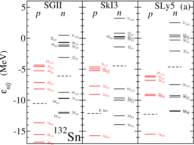
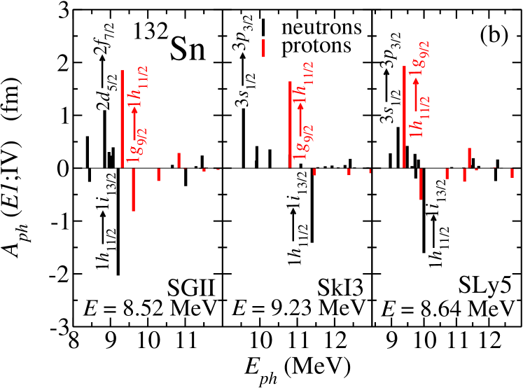
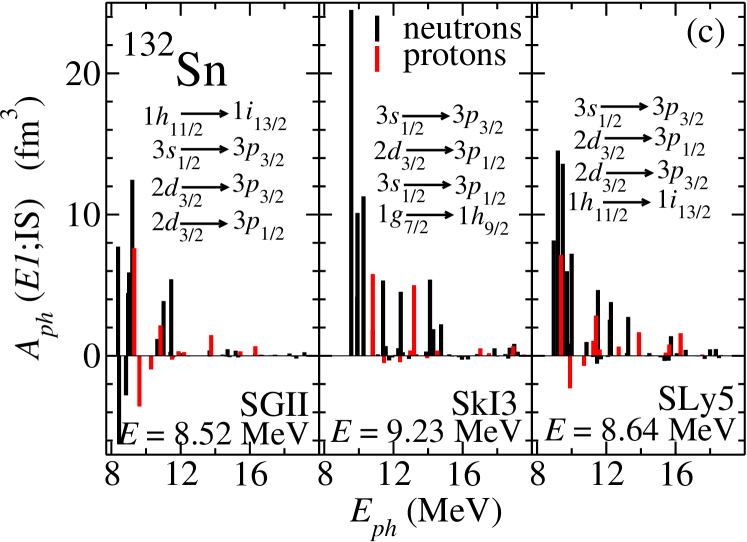
Figure 9: (Color online) Same as Fig. 8 for the case of ¹³²Sn.

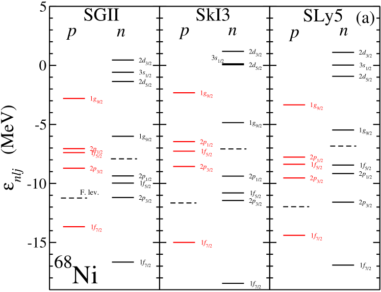
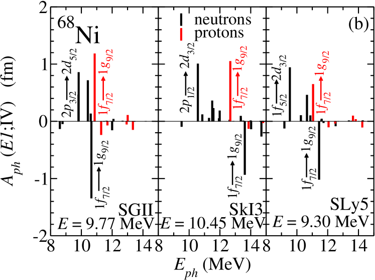
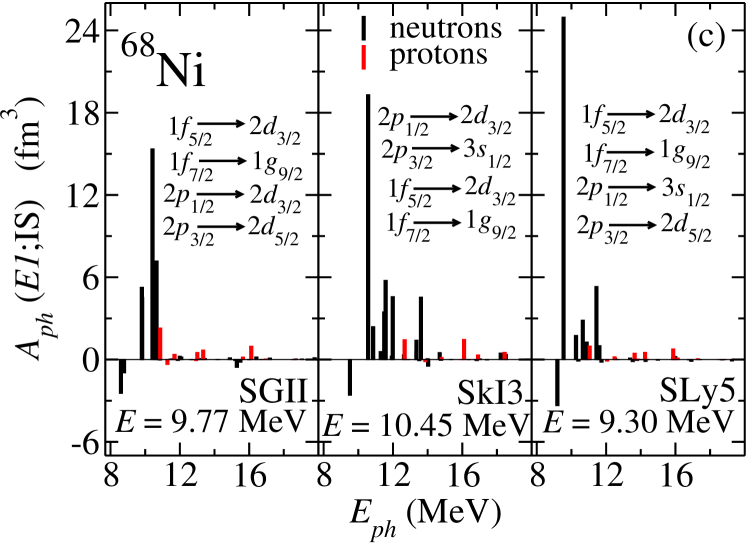
Figure 10: (Color online) Same in Fig. 8 for the case of ⁶⁸Ni.

Given the relevance of the analysis of the different reduced amplitudes $A_{ph}^{q}(E1;\xi)$, we show the same figures also for ¹³²Sn and ⁶⁸Ni where the same features found in ²⁰⁸Pb can be observed. The neutron and proton single particle levels of these nuclei are displayed in Figs. 9a and 10a, respectively. For the case of ¹³²Sn, the proton single particle levels display a similar spacing and ordering for the different models while the neutron ones do not. On the contrary, the ordering and spacing of the neutron and proton single particle levels in ⁶⁸Ni are very similar within all studied forces. This difference do not affect the qualitative structure of the isovector and isoscalar reduced amplitudes for ¹³²Sn (Figs. 9b and 9c, respectively) and ⁶⁸Ni (Figs. 10b and 10c, respectively). As in the case of ²⁰⁸Pb, while the isovector dipole responses of these nuclei do not show in the corresponding reduced amplitudes more than a few relevant neutron and proton $ph$ excitations (with some amount of destructive interference), the isoscalar reduced transition amplitudes display a more clear collective behavior of the neutron $ph$ excitations coming from the transitions of the outermost levels (see Tables 3 and 4 of the Appendix B for some numerical details).

IV Conclusions

The collective or single-particle character of the low-energy dipole response has been carefully studied in three nuclei, representative of different mass regions and neutron excess. To that end, we have analyzed within the fully self-consistent non-relativistic MF Skyrme Hartree-Fock plus RPA approach, the measured even-even nuclei ⁶⁸Ni, ¹³²Sn and ²⁰⁸Pb. In order to investigate the sensitivity of the low-energy isovector and isoscalar dipole responses of the studied nuclei on the slope of the symmetry energy, we employed three Skyrme interactions: SGII, SLy5 and SkI3. They have been selected because they cover a wide range for the predicted values of the $L$ parameter. We have qualitatively found that the isoscalar as well as the isovector dipole responses for all studied nuclei show a low-energy peak in the strength function that increases in magnitude and is shifted to larger energies with increasing values of $L$. The behavior of the isovector dipole response of these nuclei is in agreement with recent findings for which a much larger set of relativistic and non-relativistic MF interactions were used carb2010 .

From our analysis of ⁶⁸Ni, ¹³²Sn and ²⁰⁸Pb, we have also seen that the collectivity associated with the RPA states giving rise to the PDS show up depending on the nature of the probe used for exciting the nucleus: in particular, there is systematically more collectivity in the isoscalar than in the isovector transitions.

To detail this conclusion more, the studied RPA-pygmy states consistently display a strong isoscalar character, although a non negligible isovector component is always observed. Our results do not support a clear collective nature of the isovector response. This is opposite to what happens for all studied interactions when the same nuclei are excited by an isoscalar dipole operator. In this, the low-energy peak appearing in the strength function is recognizably collective and basically due to the outermost neutrons —in other words, to the neutrons forming the neutron skin known to be present in ²⁰⁸Pb prex2011 ; roca2011 and likely to developed also in ⁶⁸Ni and ¹³²Sn.

Therefore, we can conclude that the isoscalar dipole oscillations of neutron rich nuclei arising from the RPA-pygmy states can be understood within the Skyrme-HF plus RPA approach as a collective motion of the outermost neutrons in neutron rich nuclei. Such a statement should be confirmed by further experimental investigations.

Appendix A Spurious state

We subtract the spurious state from the proton ($q=p$) and neutron ($q=n$) transition densities $\delta\rho_{\nu}^{q}(r)$ [where $\nu$ characterizes the RPA state, cf. Eq. (6)] by imposing, first, that the translational operator which is proportional to the radial coordinate $r$ does not give any finite transition amplitude. This means

$$\int drr^{2}r\left(\delta\rho_{\tilde{\nu}}^{n}+\delta\rho_{\tilde{\nu}}^{p}\right)=0,$$ (14)

where $\tilde{\nu}$ denotes the corrected RPA state without spurious state contamination. As a second condition, we impose on these new transition densities that the strength of the IVGDR is not modified. That is, we write

$$\int drr^{2}r\left(\frac{Z}{A}\delta\rho_{\tilde{\nu}}^{n}-\frac{N}{A}\delta\rho_{\tilde{\nu}}^{p}\right)=\int drr^{2}r\left(\frac{Z}{A}\delta\rho_{\nu}^{n}-\frac{N}{A}\delta\rho_{\nu}^{p}\right).$$ (15)

By writing

$$\delta\rho_{\tilde{\nu}}^{q}=\delta\rho_{\nu}^{q}-\alpha^{q}\frac{d\rho_{\rm HF}^{q}(r)}{dr},$$ (16)

where $\rho_{\rm HF}^{q}(r)$ is the proton ($q=p$) or neutron ($q=n$) density obtained from the self-consistent HF calculations, we find the following solution,

$$\alpha^{n} = \frac{N}{A}\frac{\int drr^{2}\ r\delta\rho_{\nu}}{\int drr^{2}\ r\frac{d\rho_{\rm HF}^{n}}{dr}}$$ (17)

$$\alpha^{p} = \frac{Z}{A}\frac{\int drr^{2}\ r\delta\rho_{\nu}}{\int drr^{2}\ r\frac{d\rho_{\rm HF}^{p}}{dr}}$$ (18)

where $\delta\rho_{\nu}=\delta\rho_{\nu}^{n}+\delta\rho_{\nu}^{p}$.

Appendix B Most relevant $ph$ contributions

In this Appendix we give the numerical details of the most relevant $ph$ contributions to the isoscalar and isovector dipole response of ⁶⁸Ni, ¹³²Sn and ²⁰⁸Pb as predicted by SGII, SLy5 and SkI3 studied in Sec. III. Specifically, we show for all nuclei and interactions the ten neutron and proton $ph$ excitations with larger contributions to the reduced amplitude $A(E1;\xi)$ [see Eq. (3)].

Table 2: The ten largest contributions of the proton ($q=p$) and neutron ($q=n$) $ph$ excitations to the isovector and isoscalar reduced amplitudes, $A_{ph}^{q}(E1;\xi)$ where $\xi=$ IV and IS, respectively, as predicted by SGII, SLy5 and SkI3 models for ²⁰⁸Pb. The single particle levels involved in the transitions corresponding to each $ph$ excitation are also indicated.

	SGII			SkI3			SLy5
				Isovector
	$E=7.61$MeV	$A_{ph}$		$E=8.01$MeV	$A_{ph}$		$E=7.74$MeV	$A_{ph}$
		[fm]			[fm]			[fm]
$n$	$1i_{13/2}\rightarrow 1j_{15/2}$	$-2.87$		$1i_{13/2}\rightarrow 1j_{15/2}$	$-1.18$		$1i_{13/2}\rightarrow 1j_{15/2}$	$-2.02$
	$3p_{3/2}\rightarrow 3d_{5/2}$	$1.31$		$3p_{1/2}\rightarrow 4s_{1/2}$	$1.02$		$3p_{1/2}\rightarrow 4s_{1/2}$	$0.75$
	$3p_{1/2}\rightarrow 3d_{3/2}$	$0.81$		$1h_{9/2}\rightarrow 1i_{11/2}$	$-0.54$		$3p_{1/2}\rightarrow 3d_{3/2}$	$0.63$
	$1h_{9/2}\rightarrow 1i_{11/2}$	$-0.76$		$3p_{1/2}\rightarrow 3d_{3/2}$	$0.48$		$3p_{3/2}\rightarrow 3d_{5/2}$	$0.54$
	$2f_{7/2}\rightarrow 2g_{9/2}$	$0.70$		$3p_{3/2}\rightarrow 3d_{5/2}$	$0.27$		$1h_{9/2}\rightarrow 1i_{11/2}$	$-0.53$
	$2f_{5/2}\rightarrow 2g_{7/2}$	$0.53$		$3p_{3/2}\rightarrow 4s_{1/2}$	$0.26$		$3p_{3/2}\rightarrow 4s_{1/2}$	$0.33$
	$2f_{5/2}\rightarrow 3d_{3/2}$	$0.28$		$2f_{5/2}\rightarrow 3d_{3/2}$	$0.12$		$2f_{5/2}\rightarrow 3d_{3/2}$	$0.26$
	$3p_{3/2}\rightarrow 4s_{1/2}$	$0.28$		$2f_{5/2}\rightarrow 2g_{7/2}$	$0.12$		$1h_{9/2}\rightarrow 2g_{7/2}$	$0.15$
	$1h_{9/2}\rightarrow 2g_{7/2}$	$0.20$		$2f_{7/2}\rightarrow 3d_{5/2}$	$0.11$		$2f_{7/2}\rightarrow 3d_{5/2}$	$0.12$
	$3p_{1/2}\rightarrow 4s_{1/2}$	$-0.15$		$3p_{3/2}\rightarrow 3d_{3/2}$	$0.05$		$2f_{5/2}\rightarrow 2g_{7/2}$	$0.11$
$p$	$1h_{11/2}\rightarrow 1i_{13/2}$	$3.37$		$1h_{11/2}\rightarrow 1i_{13/2}$	$1.52$		$1h_{11/2}\rightarrow 1i_{13/2}$	$2.94$
	$2d_{5/2}\rightarrow 2f_{7/2}$	$-1.30$		$1g_{7/2}\rightarrow 1h_{9/2}$	$0.73$		$2d_{5/2}\rightarrow 2f_{7/2}$	$-0.93$
	$1g_{7/2}\rightarrow 1h_{9/2}$	$0.85$		$3s_{1/2}\rightarrow 3p_{1/2}$	$-0.14$		$1g_{7/2}\rightarrow 1h_{9/2}$	$0.77$
	$2d_{3/2}\rightarrow 2f_{5/2}$	$-0.69$		$2d_{5/2}\rightarrow 3p_{3/2}$	$-0.10$		$3s_{1/2}\rightarrow 3p_{3/2}$	$-0.50$
	$3s_{1/2}\rightarrow 3p_{3/2}$	$-0.38$		$2d_{5/2}\rightarrow 2f_{7/2}$	$-0.10$		$2d_{3/2}\rightarrow 2f_{5/2}$	$-0.34$
	$3s_{1/2}\rightarrow 3p_{1/2}$	$-0.19$		$2d_{3/2}\rightarrow 2f_{5/2}$	$-0.09$		$2d_{5/2}\rightarrow 3p_{3/2}$	$-0.21$
	$1g_{7/2}\rightarrow 2f_{5/2}$	$-0.19$		$2d_{3/2}\rightarrow 3p_{1/2}$	$-0.07$		$2d_{3/2}\rightarrow 3p_{1/2}$	$-0.21$
	$2d_{5/2}\rightarrow 3p_{3/2}$	$-0.15$		$3s_{1/2}\rightarrow 3p_{3/2}$	$-0.06$		$1g_{7/2}\rightarrow 2f_{5/2}$	$-0.18$
	$2d_{3/2}\rightarrow 3p_{1/2}$	$-0.13$		$1g_{7/2}\rightarrow 2f_{5/2}$	$-0.04$		$3s_{1/2}\rightarrow 3p_{1/2}$	$-0.18$
	$2d_{5/2}\rightarrow 2f_{5/2}$	$-0.06$		$1h_{11/2}\rightarrow 2g_{9/2}$	$-0.02$		$2d_{3/2}\rightarrow 3p_{3/2}$	$-0.06$
				Isoscalar
		[fm3]			[fm3]			[fm3]
$n$	$1i_{13/2}\rightarrow 1j_{15/2}$	$28.53$		$3p_{1/2}\rightarrow 4s_{1/2}$	$40.13$		$3p_{1/2}\rightarrow 4s_{1/2}$	$27.42$
	$1h_{9/2}\rightarrow 1i_{11/2}$	$12.54$		$3p_{1/2}\rightarrow 3d_{3/2}$	$11.37$		$1i_{13/2}\rightarrow 1j_{15/2}$	$17.50$
	$3p_{1/2}\rightarrow 3d_{3/2}$	$8.86$		$1i_{13/2}\rightarrow 1j_{15/2}$	$9.80$		$3p_{1/2}\rightarrow 3d_{3/2}$	$11.62$
	$2f_{5/2}\rightarrow 3d_{3/2}$	$8.57$		$3p_{3/2}\rightarrow 4s_{1/2}$	$9.64$		$3p_{3/2}\rightarrow 4s_{1/2}$	$11.16$
	$3p_{3/2}\rightarrow 3d_{5/2}$	$8.36$		$1h_{9/2}\rightarrow 1i_{11/2}$	$8.55$		$2f_{5/2}\rightarrow 3d_{3/2}$	$9.10$
	$3p_{3/2}\rightarrow 4s_{1/2}$	$6.79$		$2f_{5/2}\rightarrow 3d_{3/2}$	$4.64$		$1h_{9/2}\rightarrow 1i_{11/2}$	$8.46$
	$1h_{9/2}\rightarrow 2g_{7/2}$	$6.03$		$3p_{3/2}\rightarrow 3d_{5/2}$	$4.44$		$3p_{3/2}\rightarrow 3d_{5/2}$	$6.14$
	$2f_{7/2}\rightarrow 2g_{9/2}$	$-5.69$		$2f_{7/2}\rightarrow 3d_{5/2}$	$3.54$		$1h_{9/2}\rightarrow 2g_{7/2}$	$4.51$
	$3p_{1/2}\rightarrow 4s_{1/2}$	$-4.18$		$1h_{9/2}\rightarrow 2g_{7/2}$	$1.49$		$2f_{7/2}\rightarrow 3d_{5/2}$	$3.49$
	$2f_{5/2}\rightarrow 2g_{7/2}$	$-2.33$		$3p_{3/2}\rightarrow 3d_{3/2}$	$1.22$		$2f_{5/2}\rightarrow 3d_{5/2}$	$1.87$
$p$	$1h_{11/2}\rightarrow 1i_{13/2}$	$22.10$		$1h_{11/2}\rightarrow 1i_{13/2}$	$8.79$		$1h_{11/2}\rightarrow 1i_{13/2}$	$17.69$
	$2d_{5/2}\rightarrow 2f_{7/2}$	$-9.71$		$1g_{7/2}\rightarrow 1h_{9/2}$	$7.69$		$1g_{7/2}\rightarrow 1h_{9/2}$	$8.22$
	$1g_{7/2}\rightarrow 1h_{9/2}$	$9.20$		$2d_{5/2}\rightarrow 3p_{3/2}$	$0.82$		$2d_{5/2}\rightarrow 2f_{7/2}$	$-6.31$
	$2d_{3/2}\rightarrow 2f_{5/2}$	$-4.69$		$2d_{5/2}\rightarrow 2f_{7/2}$	$-0.65$		$1g_{7/2}\rightarrow 2f_{5/2}$	$2.81$
	$1g_{7/2}\rightarrow 2f_{5/2}$	$2.93$		$2d_{3/2}\rightarrow 3p_{1/2}$	$0.62$		$2d_{3/2}\rightarrow 2f_{5/2}$	$-2.07$
	$2d_{3/2}\rightarrow 3p_{1/2}$	$1.11$		$1h_{11/2}\rightarrow 4i_{13/2}$	$0.60$		$2d_{3/2}\rightarrow 3p_{1/2}$	$1.86$
	$2d_{5/2}\rightarrow 3p_{3/2}$	$1.10$		$1g_{7/2}\rightarrow 2f_{5/2}$	$0.59$		$2d_{5/2}\rightarrow 3p_{3/2}$	$1.70$
	$1h_{11/2}\rightarrow 4i_{13/2}$	$0.96$		$1h_{11/2}\rightarrow 2g_{9/2}$	$0.56$		$1h_{11/2}\rightarrow 2g_{9/2}$	$1.55$
	$1h_{11/2}\rightarrow 2g_{9/2}$	$0.95$		$2d_{3/2}\rightarrow 2f_{5/2}$	$-0.54$		$1g_{7/2}\rightarrow 3h_{9/2}$	$1.19$
	$1f_{5/2}\rightarrow 2g_{7/2}$	$0.92$		$1g_{7/2}\rightarrow 4h_{9/2}$	$0.46$		$1h_{11/2}\rightarrow 4i_{13/2}$	$1.07$

Table 3: Same as in Table 2 for ¹³²Sn.

	SGII			SkI3			SLy5
				Isovector
	$E=8.52$MeV	$A_{ph}$		$E=9.23$MeV	$A_{ph}$		$E=8.64$MeV	$A_{ph}$
		[fm]			[fm]			[fm]
$n$	$1h_{11/2}\rightarrow 1i_{13/2}$	$-2.02$		$1h_{11/2}\rightarrow 1i_{13/2}$	$-1.40$		$1h_{11/2}\rightarrow 1i_{13/2}$	$-1.59$
	$2d_{5/2}\rightarrow 2f_{7/2}$	$1.08$		$3s_{1/2}\rightarrow 3p_{3/2}$	$1.12$		$3s_{1/2}\rightarrow 3p_{3/2}$	$0.77$
	$3s_{1/2}\rightarrow 3p_{3/2}$	$0.59$		$1g_{7/2}\rightarrow 1h_{9/2}$	$-0.50$		$2d_{3/2}\rightarrow 3p_{1/2}$	$0.41$
	$2d_{3/2}\rightarrow 2f_{5/2}$	$0.38$		$3s_{1/2}\rightarrow 3p_{1/2}$	$0.41$		$2d_{3/2}\rightarrow 3p_{3/2}$	$0.27$
	$1g_{7/2}\rightarrow 1h_{9/2}$	$-0.33$		$2d_{3/2}\rightarrow 3p_{1/2}$	$0.34$		$3s_{1/2}\rightarrow 3p_{1/2}$	$0.26$
	$3s_{1/2}\rightarrow 3p_{1/2}$	$0.29$		$2d_{3/2}\rightarrow 2f_{5/2}$	$0.25$		$1g_{7/2}\rightarrow 1h_{9/2}$	$-0.23$
	$2d_{3/2}\rightarrow 3p_{3/2}$	$-0.25$		$2d_{5/2}\rightarrow 3p_{3/2}$	$0.16$		$2d_{5/2}\rightarrow 2f_{7/2}$	$-0.18$
	$1g_{7/2}\rightarrow 2f_{5/2}$	$0.23$		$2d_{3/2}\rightarrow 3p_{3/2}$	$0.13$		$2d_{5/2}\rightarrow 3p_{3/2}$	$0.18$
	$2d_{3/2}\rightarrow 3p_{1/2}$	$0.22$		$1g_{7/2}\rightarrow 2f_{5/2}$	$0.09$		$1g_{7/2}\rightarrow 2f_{5/2}$	$0.15$
	$1g_{7/2}\rightarrow 2f_{7/2}$	$0.07$		$2d_{5/2}\rightarrow 2f_{7/2}$	$0.07$		$2d_{3/2}\rightarrow 2f_{5/2}$	$0.15$
$p$	$1g_{9/2}\rightarrow 1h_{11/2}$	$1.84$		$1g_{9/2}\rightarrow 1h_{11/2}$	$1.63$		$1g_{9/2}\rightarrow 1h_{11/2}$	$1.92$
	$2p_{3/2}\rightarrow 2d_{5/2}$	$-0.80$		$1f_{5/2}\rightarrow 1g_{7/2}$	$0.66$		$2p_{3/2}\rightarrow 2d_{5/2}$	$-0.59$
	$1f_{5/2}\rightarrow 1g_{7/2}$	$0.27$		$2p_{3/2}\rightarrow 2d_{5/2}$	$-0.12$		$1f_{5/2}\rightarrow 1g_{7/2}$	$0.37$
	$2p_{1/2}\rightarrow 2d_{3/2}$	$-0.23$		$2p_{1/2}\rightarrow 2d_{3/2}$	$-0.12$		$2p_{1/2}\rightarrow 3s_{1/2}$	$-0.24$
	$1f_{5/2}\rightarrow 2d_{3/2}$	$-0.15$		$2p_{3/2}\rightarrow 3s_{1/2}$	$-0.10$		$2p_{1/2}\rightarrow 2d_{3/2}$	$-0.20$
	$2p_{3/2}\rightarrow 3s_{1/2}$	$-0.08$		$2p_{1/2}\rightarrow 3s_{1/2}$	$-0.08$		$1f_{5/2}\rightarrow 2d_{3/2}$	$-0.18$
	$2p_{3/2}\rightarrow 2d_{3/2}$	$-0.05$		$1f_{5/2}\rightarrow 2d_{3/2}$	$-0.05$		$2p_{3/2}\rightarrow 3s_{1/2}$	$-0.17$
	$1g_{9/2}\rightarrow 2f_{7/2}$	$-0.04$		$1g_{9/2}\rightarrow 2f_{7/2}$	$-0.04$		$1g_{9/2}\rightarrow 2f_{7/2}$	$-0.09$
	$1f_{7/2}\rightarrow 2d_{5/2}$	$-0.03$		$2p_{3/2}\rightarrow 2d_{3/2}$	$-0.03$		$1f_{7/2}\rightarrow 2d_{5/2}$	$-0.08$
	$1f_{5/2}\rightarrow 2d_{5/2}$	$-0.02$		$1f_{7/2}\rightarrow 1g_{7/2}$	$0.02$		$1f_{5/2}\rightarrow 2d_{5/2}$	$-0.03$
				Isoscalar
		[fm3]			[fm3]			[fm3]
$n$	$1h_{11/2}\rightarrow 1i_{13/2}$	$12.42$		$3s_{1/2}\rightarrow 3p_{3/2}$	$24.45$		$3s_{1/2}\rightarrow 3p_{3/2}$	$14.49$
	$3s_{1/2}\rightarrow 3p_{3/2}$	$7.69$		$2d_{3/2}\rightarrow 3p_{1/2}$	$11.25$		$2d_{3/2}\rightarrow 3p_{1/2}$	$13.55$
	$2d_{3/2}\rightarrow 3p_{3/2}$	$-6.21$		$3s_{1/2}\rightarrow 3p_{1/2}$	$10.07$		$2d_{3/2}\rightarrow 3p_{3/2}$	$8.13$
	$2d_{3/2}\rightarrow 3p_{1/2}$	$5.87$		$1g_{7/2}\rightarrow 1h_{9/2}$	$5.35$		$1h_{11/2}\rightarrow 1i_{13/2}$	$7.18$
	$1g_{7/2}\rightarrow 2f_{5/2}$	$5.37$		$1h_{11/2}\rightarrow 1i_{13/2}$	$5.29$		$3s_{1/2}\rightarrow 3p_{1/2}$	$5.95$
	$3s_{1/2}\rightarrow 3p_{1/2}$	$4.40$		$2d_{5/2}\rightarrow 3p_{3/2}$	$4.49$		$2d_{5/2}\rightarrow 3p_{3/2}$	$4.61$
	$1g_{7/2}\rightarrow 1h_{9/2}$	$3.84$		$2d_{3/2}\rightarrow 3p_{3/2}$	$4.14$		$1g_{7/2}\rightarrow 2f_{5/2}$	$3.76$
	$2d_{5/2}\rightarrow 2f_{7/2}$	$-2.76$		$1g_{7/2}\rightarrow 2f_{5/2}$	$2.19$		$1h_{11/2}\rightarrow 3g_{9/2}$	$2.71$
	$1g_{7/2}\rightarrow 2f_{7/2}$	$2.24$		$1h_{11/2}\rightarrow 3g_{9/2}$	$1.84$		$1g_{7/2}\rightarrow 1h_{9/2}$	$2.51$
	$2d_{5/2}\rightarrow 3p_{3/2}$	$1.15$		$2d_{3/2}\rightarrow 2f_{5/2}$	$1.81$		$1g_{9/2}\rightarrow 2f_{7/2}$	$1.35$
$p$	$1g_{9/2}\rightarrow 1h_{11/2}$	$7.59$		$1g_{9/2}\rightarrow 1h_{11/2}$	$5.75$		$1g_{9/2}\rightarrow 1h_{11/2}$	$7.10$
	$2p_{3/2}\rightarrow 2d_{5/2}$	$-3.55$		$1f_{5/2}\rightarrow 1g_{7/2}$	$4.96$		$1f_{5/2}\rightarrow 1g_{7/2}$	$2.81$
	$1f_{5/2}\rightarrow 1g_{7/2}$	$2.12$		$1g_{9/2}\rightarrow 2f_{7/2}$	$0.64$		$2p_{3/2}\rightarrow 2d_{5/2}$	$-2.26$
	$1f_{5/2}\rightarrow 2d_{3/2}$	$1.43$		$1f_{5/2}\rightarrow 2d_{3/2}$	$0.48$		$1f_{5/2}\rightarrow 2d_{3/2}$	$1.63$
	$2p_{1/2}\rightarrow 2d_{3/2}$	$-0.92$		$2p_{3/2}\rightarrow 2d_{5/2}$	$-0.47$		$1g_{9/2}\rightarrow 2f_{7/2}$	$1.56$
	$1g_{9/2}\rightarrow 2f_{7/2}$	$0.64$		$2p_{1/2}\rightarrow 2d_{3/2}$	$-0.41$		$2p_{1/2}\rightarrow 3s_{1/2}$	$1.02$
	$1g_{9/2}\rightarrow 4h_{11/2}$	$0.41$		$1g_{9/2}\rightarrow 4h_{11/2}$	$0.40$		$1f_{7/2}\rightarrow 3g_{9/2}$	$0.80$
	$1f_{5/2}\rightarrow 4g_{7/2}$	$0.34$		$1f_{5/2}\rightarrow 4g_{7/2}$	$0.38$		$1g_{9/2}\rightarrow 4h_{11/2}$	$0.78$
	$1d_{3/2}\rightarrow 2f_{5/2}$	$0.33$		$1g_{9/2}\rightarrow 5h_{11/2}$	$0.35$		$1f_{7/2}\rightarrow 2d_{5/2}$	$0.76$
	$1f_{7/2}\rightarrow 3g_{9/2}$	$0.28$		$2p_{1/2}\rightarrow 3s_{1/2}$	$0.33$		$1d_{5/2}\rightarrow 2f_{7/2}$	$0.69$

Table 4: Same as in Table 2 for ⁶⁸Ni.

	SGII			SkI3			SLy5
				Isovector
	$E=9.77$MeV	$A_{ph}$		$E=10.45$MeV	$A_{ph}$		$E=9.30$MeV	$A_{ph}$
		[fm]			[fm]			[fm]
$n$	$1f_{7/2}\rightarrow 1g_{9/2}$	$-1.34$		$2p_{1/2}\rightarrow 2d_{3/2}$	$1.00$		$1f_{7/2}\rightarrow 1g_{9/2}$	$-1.01$
	$2p_{3/2}\rightarrow 2d_{5/2}$	$0.85$		$1f_{7/2}\rightarrow 1g_{9/2}$	$-0.92$		$1f_{5/2}\rightarrow 2d_{3/2}$	$0.93$
	$1f_{5/2}\rightarrow 2d_{3/2}$	$0.71$		$2p_{3/2}\rightarrow 2d_{5/2}$	$0.35$		$2p_{3/2}\rightarrow 2d_{5/2}$	$0.45$
	$2p_{1/2}\rightarrow 2d_{3/2}$	$0.46$		$1f_{5/2}\rightarrow 2g_{7/2}$	$-0.26$		$2p_{1/2}\rightarrow 3s_{1/2}$	$-0.12$
	$1f_{5/2}\rightarrow 1g_{7/2}$	$-0.15$		$2p_{3/2}\rightarrow 3s_{1/2}$	$0.22$		$2p_{1/2}\rightarrow 2d_{3/2}$	$0.10$
	$2p_{3/2}\rightarrow 3s_{1/2}$	$0.13$		$1f_{5/2}\rightarrow 2d_{3/2}$	$0.18$		$1f_{5/2}\rightarrow 3d_{3/2}$	$0.09$
	$1f_{5/2}\rightarrow 2d_{5/2}$	$-0.12$		$1f_{5/2}\rightarrow 1g_{7/2}$	$-0.13$		$1f_{5/2}\rightarrow 2g_{7/2}$	$-0.08$
	$2p_{1/2}\rightarrow 3s_{1/2}$	$-0.04$		$1f_{5/2}\rightarrow 2d_{5/2}$	$0.11$		$1f_{5/2}\rightarrow 2d_{5/2}$	$-0.05$
	$1f_{5/2}\rightarrow 3d_{3/2}$	$0.03$		$2p_{1/2}\rightarrow 3s_{1/2}$	$-0.09$		$2p_{3/2}\rightarrow 3s_{1/2}$	$0.04$
	$1f_{7/2}\rightarrow 2d_{5/2}$	$-0.03$		$1f_{5/2}\rightarrow 3d_{3/2}$	$0.09$		$1f_{5/2}\rightarrow 1g_{7/2}$	$-0.02$
$p$	$1f_{7/2}\rightarrow 1g_{9/2}$	$1.18$		$1f_{7/2}\rightarrow 1g_{9/2}$	$1.04$		$1f_{7/2}\rightarrow 1g_{9/2}$	$0.64$
	$2s_{1/2}\rightarrow 2p_{3/2}$	$-0.23$		$1d_{3/2}\rightarrow 1f_{5/2}$	$0.31$		$1d_{3/2}\rightarrow 2p_{1/2}$	$-0.10$
	$1d_{3/2}\rightarrow 2p_{1/2}$	$-0.14$		$2s_{1/2}\rightarrow 2p_{3/2}$	$-0.12$		$2s_{1/2}\rightarrow 2p_{3/2}$	$-0.10$
	$1d_{3/2}\rightarrow 1f_{5/2}$	$0.10$		$1d_{3/2}\rightarrow 2p_{1/2}$	$-0.07$		$1d_{3/2}\rightarrow 1f_{5/2}$	$0.09$
	$1f_{7/2}\rightarrow 2d_{5/2}$	$-0.07$		$1f_{7/2}\rightarrow 2d_{5/2}$	$-0.03$		$1f_{7/2}\rightarrow 2d_{5/2}$	$-0.06$
	$1d_{3/2}\rightarrow 2p_{3/2}$	$-0.06$		$1d_{3/2}\rightarrow 2p_{3/2}$	$-0.02$		$1d_{3/2}\rightarrow 2p_{3/2}$	$-0.03$
	$2s_{1/2}\rightarrow 2p_{1/2}$	$-0.05$		$1d_{5/2}\rightarrow 1f_{5/2}$	$0.01$		$2s_{1/2}\rightarrow 2p_{1/2}$	$0.03$
	$1d_{5/2}\rightarrow 2p_{3/2}$	$-0.03$		$1f_{7/2}\rightarrow 2g_{7/2}$	$0.01$		$1d_{5/2}\rightarrow 2p_{3/2}$	$-0.02$
	$1d_{5/2}\rightarrow 1f_{5/2}$	$0.01$		$1d_{5/2}\rightarrow 2p_{3/2}$	$-0.01$		$1d_{5/2}\rightarrow 1f_{5/2}$	$0.01$
	$1f_{7/2}\rightarrow 1g_{7/2}$	$0.01$		$2s_{1/2}\rightarrow 2p_{1/2}$	$0.01$		$1f_{7/2}\rightarrow 1g_{7/2}$	$0.01$
				Isoscalar
		[fm3]			[fm3]			[fm3]
$n$	$1f_{5/2}\rightarrow 2d_{3/2}$	$15.35$		$2p_{1/2}\rightarrow 2d_{3/2}$	$19.31$		$1f_{5/2}\rightarrow 2d_{3/2}$	$24.96$
	$1f_{7/2}\rightarrow 1g_{9/2}$	$7.17$		$2p_{3/2}\rightarrow 3s_{1/2}$	$5.76$		$1f_{7/2}\rightarrow 1g_{9/2}$	$5.32$
	$2p_{1/2}\rightarrow 2d_{3/2}$	$5.26$		$1f_{5/2}\rightarrow 2d_{3/2}$	$4.58$		$2p_{1/2}\rightarrow 3s_{1/2}$	$-3.36$
	$2p_{3/2}\rightarrow 2d_{5/2}$	$4.51$		$1f_{7/2}\rightarrow 1g_{9/2}$	$4.55$		$2p_{3/2}\rightarrow 2d_{5/2}$	$2.86$
	$2p_{3/2}\rightarrow 3s_{1/2}$	$2.56$		$2p_{3/2}\rightarrow 2d_{5/2}$	$3.46$		$2p_{1/2}\rightarrow 2d_{3/2}$	$1.76$
	$1f_{5/2}\rightarrow 2d_{5/2}$	$-2.46$		$2p_{1/2}\rightarrow 3s_{1/2}$	$-2.60$		$1f_{5/2}\rightarrow 3d_{3/2}$	$1.26$
	$2p_{1/2}\rightarrow 3s_{1/2}$	$-0.96$		$1f_{5/2}\rightarrow 2d_{5/2}$	$2.39$		$1f_{5/2}\rightarrow 2d_{5/2}$	$-1.05$
	$1f_{7/2}\rightarrow 2d_{5/2}$	$-0.56$		$1f_{5/2}\rightarrow 3d_{3/2}$	$1.40$		$2p_{3/2}\rightarrow 3s_{1/2}$	$1.00$
	$1f_{5/2}\rightarrow 1g_{7/2}$	$0.23$		$2p_{3/2}\rightarrow 4s_{1/2}$	$0.60$		$1f_{7/2}\rightarrow 5g_{9/2}$	$0.23$
	$2p_{3/2}\rightarrow 5d_{5/2}$	$0.22$		$2p_{1/2}\rightarrow 4s_{1/2}$	$0.57$		$1f_{7/2}\rightarrow 4g_{9/2}$	$0.22$
$p$	$1f_{7/2}\rightarrow 1g_{9/2}$	$2.29$		$1d_{3/2}\rightarrow 1f_{5/2}$	$1.46$		$1f_{7/2}\rightarrow 1g_{9/2}$	$0.98$
	$1f_{7/2}\rightarrow 2d_{5/2}$	$0.96$		$1f_{7/2}\rightarrow 1g_{9/2}$	$1.44$		$1f_{7/2}\rightarrow 2d_{5/2}$	$0.77$
	$1d_{3/2}\rightarrow 2p_{1/2}$	$0.68$		$1f_{7/2}\rightarrow 2d_{5/2}$	$0.52$		$1d_{3/2}\rightarrow 2p_{1/2}$	$0.51$
	$1d_{3/2}\rightarrow 1f_{5/2}$	$0.50$		$1d_{3/2}\rightarrow 2p_{1/2}$	$0.33$		$1d_{3/2}\rightarrow 1f_{5/2}$	$0.46$
	$1d_{3/2}\rightarrow 2p_{3/2}$	$0.37$		$1f_{7/2}\rightarrow 5g_{9/2}$	$0.29$		$1f_{7/2}\rightarrow 5g_{9/2}$	$0.36$
	$2s_{1/2}\rightarrow 2p_{3/2}$	$-0.35$		$1f_{7/2}\rightarrow 6g_{9/2}$	$0.22$		$1f_{7/2}\rightarrow 4g_{9/2}$	$0.26$
	$1f_{7/2}\rightarrow 5g_{9/2}$	$0.34$		$1f_{7/2}\rightarrow 4g_{9/2}$	$0.19$		$1f_{7/2}\rightarrow 6g_{9/2}$	$0.22$
	$1f_{7/2}\rightarrow 4g_{9/2}$	$0.23$		$1d_{3/2}\rightarrow 5f_{5/2}$	$0.16$		$1d_{3/2}\rightarrow 2p_{3/2}$	$0.20$
	$1f_{7/2}\rightarrow 6g_{9/2}$	$0.22$		$1d_{5/2}\rightarrow 4f_{7/2}$	$0.15$		$1d_{5/2}\rightarrow 4f_{7/2}$	$0.18$
	$1d_{5/2}\rightarrow 4f_{7/2}$	$0.19$		$1d_{3/2}\rightarrow 2p_{3/2}$	$0.14$		$1d_{3/2}\rightarrow 4f_{5/2}$	$0.17$

References

- (1) P. F. Bortignon, A. Bracco, and R. A. Broglia, Giant Resonances. Nuclear Structure at Finite temperature (Harwood Ac. Publ., New York, 1998).
- (2) M. N. Harakeh and A. M. Van Der Woude, Giant Resonances: Fundamental High-Frequency Modes of Nuclear Excitations (Oxford University Press, Oxford, 2001).
- (3) N. Paar, D. Vretenar, E. Khan, and Gianluca Colò, Rep. Prog. Phys. 70 691 (2007).
- (4) J. Blaizot, J. F. Berger, J. Dechargé, and M. Girod Nucl. Phys. A 591, 435 (1995).
- (5) B. K. Agrawal, S. Shlomo, and V. Kim Au, Phys. Rev. C 68, 031304 (2003).
- (6) G. Colò, N. Van Giai, J. Meyer, K. Bennaceur, and P. Bonche Phys. Rev. C 70, 024307 (2004).
- (7) B. G. Todd-Rutel and J. Piekarewicz, Phys. Rev. Lett. 95, 122501 (2005).
- (8) P. G. Reinhard, Nucl. Phys. A 649, 305c (1999).
- (9) L. Trippa, G. Colò, and E. Vigezzi Phys. Rev. C 77, 061304(R) (2008).
- (10) I. Tanhihata, Prog. Part. Nucl. Phys. 35, 505 (1995).
- (11) H. Geissel, G. Müzenberg, and R. Riisager, Annu. Rev. Nucl. Part. Sci. 45, 163 (1995).
- (12) A. Mueller, Prog. Part. Nucl. Phys. 46, 359 (2001).
- (13) A. Klimkiewicz et al., Phys. Rev. C 76, 051603(R) (2007).
- (14) A. Leistenschneider et al. Phys. Rev. Lett. 86 5442 (2001).
- (15) T. Hartmann et al. Phys. Rev. Lett. 85 274 (2000).
- (16) T. Hartmann et al. Phys. Rev. Lett. 93 192501 (2004).
- (17) O. Wieland et. al., Phys. Rev. Lett. 102 092502 (2009).
- (18) P. Adrich et. al., Phys. Rev. Lett. 95 132501 (2005).
- (19) S. C. Fultz et al., Phys. Rev. 186, 1255 (1969).
- (20) N. Ryezayeva et al., Phys. Rev. Lett. 89, 272502 (2002).
- (21) Tsunenori Inakura, Takashi Nakatsukasa, and Kazuhiro Yabana, Phys. Rev. C 84, 021302(R) (2011).
- (22) A.Carbone et al., Phys. Rev. C 81, 041301 (2010).
- (23) J. Piekarewicz, Phys. Rev. C 83 034319 (2011).
- (24) P.-G. Reinhard and W. Nazarewicz, Phys. Rev. C 81, 051303 (2010).
- (25) D. Gambacurta, M. Grasso, and F. Catara, Phys. Rev. C 84 034301 (2011).
- (26) V.Baran, B. Frecus, M. Colonna, and M. Di Toro, arXiv:1111.6504v1.
- (27) E. Yüksel, E. Khan, and K. Bozkurt, Submited to Nucl. Phys. A
- (28) J. M. Lattimer and M. Prakash, Astrophys. J. 550, 426 (2001); Science 304, 536 (2004).
- (29) X. Roca-Maza and J. Piekarewicz, Phys. Rev. C 78, 025807 (2008).
- (30) B. A. Brown, Phys. Rev. Lett. 85, 5296 (2000).
- (31) M. Centelles, X. Roca-Maza, X. Viñas, M. Warda, Phys. Rev. Lett. 102, 122502 (2009)
- (32) X. Roca-Maza, M. Centelles, X. Viñas, M. Warda, Phys. Rev. Lett. 106, 252501 (2011)
- (33) P.-G. Reinhard and W. Nazarewicz, private communication.
- (34) D. Vretenar et al., Nuc. Phys. A 692, 496 (2001).
- (35) M. Urban, arXiv:1103.0861v2
- (36) M. Bender, P.-H. Heenen, and P.-G. Reinhard, Rev. Mod. Phys. 75, 121 (2003).
- (37) D. Vretenar, A. V. Afanasjev, G. A. Lalazissis, and P. Ring, Phys. Rep. 409, 101 (2005).
- (38) N. Van Giai and H. Sagawa, Phys. Lett. B 106, 379 (1981).
- (39) E. Chabanat et al., Nucl. Phys. A 635, 231 (1998); Nucl. Phys. A 643, 441 (1998).
- (40) P.-G. Reinhard and H. Flocard, Nucl. Phys. A 584, 467 (1995).
- (41) D. Vautherin and D. M. Brink, Phys. Rev. C 5, 626 (1972).
- (42) M. Beiner, H. Flocard, N. Van Giai and P. Quentin, Nucl. Phys. A 238, 29 (1975).
- (43) P. Ring and P. Schuck, The Nuclear Many-Body Problem (Springer-Verlag, New York, 1980).
- (44) D. J. Rowe, Nuclear Collective Motion (Methuen and Co. Ltd., London, 1980).
- (45) S. Fracasso and G. Colò, Phys. Rev. C 72, 064310 (2005).
- (46) T. Sil, S. Shlomo, B.K. Agrawal, and P.-G. Reinhard, Phys. Rev. C 73, 034316 (2006).
- (47) A. Bohr and B.R. Mottelson, Nuclear Structure, vol. I (W.A. Benjamin, Reading, 1969).
- (48) G. Coló et al. Submitted to Comp. Phys. Comm.
- (49) Kazuhito Mizuyama, and Gianluca Colò arXiv:1108.2161.
- (50) N. Van Giai and H. Sagawa, Nucl. Phys. A 371, 1 (1981).
- (51) D. Sarchi, P.F. Bortignon, G. Colò, Phys. Lett. B 601 27 (2004).
- (52) E. Litvinova, P. Ring, D. Vretenar, Phys. Lett. B 647 111 (2007).
- (53) G. Tertychny et al., Phys. Lett. B 647 104 (2007).
- (54) P. Papakonstantinou, H. Hergert V. Yu. Ponomarev, and R. Roth, arxiv:1110.0973v1 (2011)
- (55) N.Paar, Y. F. Niu, D. Vretenar, and J. Meng, Phys. Rev. Lett. 103, 032502 (2009).
- (56) U. Garg, Nucl. Phys. A 649, 66c (1999).
- (57) B. L. Berman and S. C. Fultz, Rev. Mod. Phys. 47, 713 (1975).
- (58) J. Endres et. al., Phys. Rev. Lett. 105, 212503 (2010)
- (59) K. Kumar, P. A. Souder, R. Michaels, and G. M. Urciuoli, http://hallaweb.jlab.org/parity/prex (see section “Status and Plans” for latest updates).