Supervised Learning of Logical Operations in Layered Spiking Neural Networks with Spike Train Encoding

Abstract

Few algorithms for supervised training of spiking neural networks exist that can deal with patterns of multiple spikes, and their computational properties are largely unexplored. We demonstrate in a set of simulations that the ReSuMe learning algorithm can be successfully applied to layered neural networks. Input and output patterns are encoded as spike trains of multiple precisely timed spikes, and the network learns to transform the input trains into target output trains. This is done by combining the ReSuMe learning algorithm with multiplicative scaling of the connections of downstream neurons.

We show in particular that layered networks with one hidden layer can learn the basic logical operations, including Exclusive-Or, while networks without hidden layer cannot, mirroring an analogous result for layered networks of rate neurons.

While supervised learning in spiking neural networks is not yet fit for technical purposes, exploring computational properties of spiking neural networks advances our understanding of how computations can be done with spike trains.

Keywords:Spiking Neural Networks, Supervised Learning, Logical Operation, Spike Trains

1 Introduction

Artificial neural networks are developed both as models of neural processing in nervous systems and as learning devices in artificial intelligence. Neural networks of rate neurons have found ample applications in industry because efficient general purpose learning algorithms exist. In our understanding, a general purpose algorithm can learn arbitrary mappings of input-output pattern pairs, – subject to general constraints of whether the input-output mapping is representable in the network or crosstalk between similar input patterns [13, 1]. Examples of such general-purpose algorithms for rate neurons are the family of backpropagation algorithms [25]. However networks of rate neurons are not biologically plausible as they do not show spiking behaviour.

On the other hand, spiking neural networks are biologically more plausible and serve mainly as models of nervous processing, but general purpose learning algorithms – in the way backpropagation is applied to rate neurons – have not yet been found [10]. A general-purpose learning algorithm for spiking networks should be able to map arbitrary spatio-temporal input spike patterns to arbitrary output spike patterns. So far learning in these spiking networks is largely correlation-based, that is variants of Hebbian learning such as Spike-Timing-Dependent Plasticity (STDP) are typically used to change synaptic weights [12].

In this paper we will present a series of simulations involving layered feedforward networks of spiking neurons and demonstrate that these are able to learn simple computations in a supervised way. We will use an encoding of input and output patterns that makes use of spike trains with strict spike times. In comparable settings, so far only classification tasks or simple mapping tasks have been considered [9, 14, 21, 11], either with only a single neuron or in much larger Liquid State Machines [15], but no computational tasks. Or computational tasks like the Exclusive-Or problem have been considered in layered networks, but only with single-spike latency-encoded outputs [3, 4, 30, 29]. In contrast, it is our aim to demonstrate that layered networks can learn to perform simple, but non-trivial computations in a supervised framework and make use of multiple timed spikes for input and output patterns.

In particular, as basic building blocks of computation, we demonstrate that these networks can learn logical operations when logical values false and true are encoded as spike trains both for inputs and outputs. While it can often be shown that (hand-coded) spiking neural networks can be Turing-equivalent [15, 28], it is instructive to demonstrate that basic building blocks of such computations can indeed be learnt. Already for rate neurons, theoretical Turing equivalence and practical learnability of a problem may not coincide [2, 8].

A key problem in neuroscience is to understand the neural code. Usually the approach is “bottom-up”, that is spike trains are recorded and later analysed and checked for correlations in rate and timing with experimental conditions, for example sensory stimuli [17]. However many areas of a nervous system might be so far remote from direct sensory stimuli, that it is difficult to detect such correlations and to understand what precise computational function a natural network implements and how.

Therefore, besides as an initial step towards general-purpose learning for spiking neural networks, the present article may also be seen as a top-down complement of these neuroscientific approaches. Under biologically inspired constraints on information processing, we explore whether simple types of computation can be performed with spike-train based encoding. While bio-inspired, our approach however takes into account neuroscientific detail on a coarse level only.

The article is structured as follows: In the next section 2 we discuss basic properties of two learning algorithms for spiking neurons and motivate our choice of ReSuMe. We present our learning task in section 3. In section 4 we describe the details of the simulation setup. Section 5 presents and discusses a series of simulations on logical operations. In section 6 we conclude by embedding the results into their wider context.

2 Background

Recently there have been interesting developments regarding supervised learning algorithms for spiking neural networks. Notably, there are the SpikeProp learning algorithm [3, 4] and ReSuMe [21].

While SpikeProp has been applied to layered feedforward networks, each neuron is restricted to only one spike during a certain period. Similar restrictions also apply to extensions of this algorithm [30, 4]. SpikeProp essentially is a gradient-descent algorithm similar to backpropagation for rate neurons. While rate neuron backpropagation uses the minimisation of Euclidean distance between actual and target output activation to derive weight changes to minimise error, in SpikeProp the Euclidean distance of actual and target spike times plays the same role. As in standard backpropagation, SpikeProp weight changes for synaptic connections between neurons are given by the (anti-)gradient of the overall network error with respect to the weight. Such gradient descent algorithms overcome the credit assignment problem by utilising the chain rule of differentiation to derive error signals for downstream neurons.

Applications of SpikeProp and its extensions have mainly been to classification tasks in layered networks where the early or late timing of a single output spike indicates the class [4, 30, 26]. SpikeProp’s application to the non linearly separable Exclusive-OR problem also follows this pattern [3]. Generally for SpikeProp-based algorithms, it is crucial that hidden layer neurons are initialised such that they spike at least once for all patterns or no error signals for that neuron and its weight arise. In this sense, it is difficult to come up with a good weight initialisation independent of the task and the pattern encoding used [26].

Finally, Booij and tat Nguyen [4] suggest an extension of SpikeProp where multiple spikes are allowed in the hidden and input layers. They claim their extension is in principle also applicable for multiple output spikes, but – to our knowledge – it has never been successfully applied to any such task experimentally. Also our own preliminary simulations with SpikeProp failed for multiple output spikes. Therefore simulations in the paper will be based on ReSuMe, see section 4.3.

ReSuMe is motivated by an analogue of the $\delta$-rule and is based on STDP [21]. From a combination of an STDP process between target and input spike trains of a neuron and an anti-STDP process between the actual output train and the input, it derives a differential STDP rule that is used to generate weight changes for the synaptic connections into a neuron.

This algorithm is capable of training a single neuron to reproduce an arbitrary prescribed target spike train via supervised learning; however it needs a large number of incoming spikes to do so successfully [21]. Unlike SpikeProp, ReSuMe is able to deal with spike patterns that involve many spikes. However it can only be applied to neurons that have a direct target spike train assigned, and the credit assignment for downstream neurons is circumvented by either training single neurons or a layer of output neurons on top of a large immutable LSM [15]. Experimental tasks include, for example, single neurons (or sets) producing a prescribed spike train from their incoming spikes, or classifying spike patterns when trained neurons are used as readouts for a LSM [21].

However, much smaller networks, similar to the layered feedforward networks used for SpikeProp can also perform computations and transform spike trains as will be demonstrated in this article. Hence ReSuMe has the potential to be a general-purpose learning algorithm for patterns that are based on (arbitrary) spike trains.

3 Task Overview

This section is an overview of the learning task, the encoding and the network structure used. For details, see the section 4. We concentrate on simple logical operations . These are simpler than real world data, but it is also much clearer what type of computation has to be learnt in the network. We are primarily interested in these simulations as a proof of concept that computation with spike trains is possible, but logical operations are also at the heart of every symbolic computation, and it is instructive to analyse whether these basic building blocks can be learnt.

Let $J_{0}$ and $J_{1}$ denote the inputs to a logical operation and $Q$ its output. Truth values false and true both for input and output will be encoded as spike trains for a layered feedforward network [23] of spiking neurons (see fig. 1). For the single output neuron $Q$ (in slight abuse of notation), there are two target spikes trains $S_{\textsc{true}}$ and $S_{\textsc{false}}$, standing for the two logical output values. For the inputs, the network has two equally sized banks $J_{0}$ and $J_{1}$ of input neurons. Each bank plays the role of one logical input to the network. For each bank $J_{i}$ the list of given spike trains for the bank’s individual neurons $(S)_{J_{i},\textsc{true}}$ or $(S)_{J_{i},\textsc{false}}$ denote collectively the logical value input to this bank. For details of spike train choice, see section 4.6.

We have chosen to train the four operations TRUE, J0, AND and XOR. As spike trains are assigned randomly to their interpretations of false and true and to their bank, but have otherwise identical properties, these four cases cover all 16 possible logical operations of two binary variables [5]. For example OR can be derived from AND if logical values of all input and target spike trains are inverted. TRUE and J0 might seem trivial from a logic point of view, but they are probably not for a spiking neural network:

TRUE is the logical operation that always has true as output, irrespective of its inputs. It tests whether the network can produce the same (or at least a similar) output train for dissimilar sets of input trains.

J0 is the logical operation that always has the same value as its $J_{0}$ input. It tests whether the network can ignore the input from bank $J_{1}$ which effectively is just noise in this task.

AND. The logical conjunction is linearly separable, can therefore be learned in a single layer preceptron, and is viewed as a simple computation to learn.

XOR. The Exclusive-Or operation is not linearly separable and is therefore considered more difficult to learn than AND. It cannot be learnt with a simple preceptron and has frequently been used to demonstrate the power of a learning algorithm [16]

(a) Network structure.

(b) Logical Operation.

Figure 1: Network structure and encoding of logical values. (a) A three-layer network with input, hidden and output layer. The input layer consists of two banks $J_{0}$ and $J_{1}$. All neurons in a bank collectively serve as one logical input. The firing pattern of neuron $Q$ represents the output value. $\Uparrow$ stands for the feedforward connections between layers. (b) Logical operations with spike trains. A logical value false or true is encoded in a set of spike trains, and these are applied to the input banks $J_{0}$ and $J_{1}$. The network learns to perform a logical operation (such as XOR) and produces an output spike train which then needs to be interpreted as a logical value.

4 Methods

In this section we describe and motivate our experimental setup in more detail.

ReSuMe is a supervised learning algorithm for single spiking neurons usually driven by a large number of input spike trains [21]. ReSuMe is not fixed to a particular neuron type, but – as STDP – implicitly assumes, at least on longer time scales, that recent inputs have more influence on the current activation of a neuron than past inputs. We present the general network structure, fix a convenient notation and introduce ReSuMe in a form suitable for easy implementation with discrete time steps as opposed to the integral formulation in continuous time in [21]. We also address the problem of weight initialisation for downstream neurons.

4.1 Networks

We consider layered feedforward networks [23]. Although they are only feedforward and not recurrent, they have a temporal dimension since they use spiking neurons and spike train dynamics play out in time. Our simulations used networks with two (input, output) and three layers (input, hidden and output). The two-layered networks are similar to the ones used for ReSuMe [21] and the three layered ones are similar to the ones used with SpikeProp [3].

Neurons within layers do not connect to each other, but fully connect to the subsequent layer: there are multiple connections $w_{XY,s}$ for all delays $s=1\mathrm{m}\mathrm{s}\cdots 10\mathrm{m}\mathrm{s}$ from any neuron $X$ in the present layer to any neuron $Y$ in the subsequent layer. The output layer consists of just a single neuron, and the input layer consists of “dummy” neurons (without any dynamics) which simply serve to feed input spike trains into the next layer.

The connections between the input and output layer for the two-layered networks are subject to ReSuMe learning (eq. 1 and eq. 2). In the three-layer network only the connections from the hidden layer to the output layer are subject to ReSuMe learning, while connections from the input layer to the hidden layer are subject to rate adjustment according to eq. 4, further down.

ReSuMe needs a large number (hundreds) of incoming connections to function [21], we (like in SpikeProp) instead use fewer inputs, but multiply incoming connections by having 10 weights with different delays between any two neurons, so effectively we also achieve a high number of incoming spikes to any neuron.

4.2 Notation

Let $S_{X}$ denote the output spike train from neuron $X$. We understand the spike train as the ordered set of spike times $t_{i}$ of $X$, ie $S_{X}=(t_{i})$. A neuron $X$ undergoing supervised learning will have two output spike trains associated with it, namely the train of actual spikes $S_{X}^{(a)}=(t_{i}^{(a)})$, that is the list of times $t_{i}^{(a)}$ when it did actually spike, and the train $S_{X}^{(d)}=(t_{i}^{(d)})$ of desired spike times $t_{i}^{(d)}$ when we want it to spike. Let $w_{XY}$ denote the weight of the synaptic connection from presynaptic neuron $X$ to postsynaptic neuron $Y$. We distinguish multiple synaptic connections between the same neurons $X$ and $Y$ with different delays $s$ by an additional index, that is $w_{XY,s}$. If clear from the context which particular quantity we refer to or if the argumentation is generic, we will leave out indices on weights $w_{XY}$, times $t_{i}$ and on other quantities introduced later.

4.3 Weight Changes in ReSuMe

ReSuMe considers a single neuron $Y$ that is driven by a number of incoming spike trains, either as direct input spike trains or trains from other neurons. It introduces a differential STDP process involving the desired and actual output spike trains $S^{(d)}_{Y}$ and $S^{(a)}_{Y}$ and all input spike trains. We refer the reader to details of its derivation in [21] and present a formulation of ReSuMe that is broken down to the effects of individual input-output spike pairs.

More precisely, for each connection $w_{XY}$ there is an STDP process between the corresponding input train $S_{X}$ and the desired output train $S_{Y}^{(d)}$. This process is complemented by an anti-STDP process between the same incoming train $S_{X}$ and the actual output train $S_{Y}^{(a)}$. These processes can be formulated quite generally with a number of parameters, however, we restrict ourselves here to a formulation with a reduced set of parameters where contributions of the two STDP processes are of equal magnitude.

The total weight change $\Delta w_{XY}$ resulting from the STDP processes between the trains is the sum of all contributions of individual input-output spike pairs $(t_{X},t^{(d)}_{Y})\in S_{X}\times S_{Y}^{(d)}$ and $(t_{X},t^{(a)}_{Y})\in S_{X}\times S_{Y}^{(a)}$ as follows:

$$\Delta w_{XY}^{(d)}(t_{X},t_{Y}^{(d)})=a_{d}+\begin{cases}+A_{di}e^{-\frac{t_{Y}^{(d)}-t_{X}}{\tau}},&t_{Y}^{(d)}-t_{X}\geq 0\\ -A_{id}e^{\frac{t_{Y}^{(d)}-t_{X}}{\tau}},&t_{Y}^{(d)}-t_{X}<0\end{cases}$$ (1)

with constants $a_{d},A_{di},A_{id},\tau\geq 0$. Similarly, the anti-STDP process between an input train and the actual output train effects weight changes as

$$\Delta w_{XY}^{(a)}(t_{X},t_{Y}^{(a)})=-a_{d}+\begin{cases}-A_{di}e^{-\frac{t_{Y}^{(a)}-t_{X}}{\tau}},&t_{Y}^{(a)}-t_{X}\geq 0\\ +A_{id}e^{\frac{t_{Y}^{(a)}-t_{X}}{\tau}},&t_{Y}^{(a)}-t_{X}<0\end{cases}.$$ (2)

With constants chosen the same as in eq. 1, $\Delta w^{(a)}(t_{X},t_{Y})=-\Delta w^{(d)}(t_{X},t_{Y})$ so that the two processes are balanced. If the desired and actual spike times coincide, there is no further weight change resulting from such a pair. The total weight change of $w_{XY}$ from spike trains $S_{X},S_{Y}^{(a)}$ and $S_{Y}^{(d)}$ is the sum of all above contributions from all pairings of (desired and actual) output and input spikes:

$$\Delta w_{XY}=\sum_{t_{X}\in S_{X}}\left(\sum_{t^{(d)}\in S^{(d)}_{Y}}\Delta w_{XY}^{(d)}(t_{X},t^{(d)})+\sum_{t^{(a)}\in S^{(a)}_{Y}}\Delta w_{XY}^{(a)}(t_{X},t^{(a)})\right)$$ (3)

If connections $w_{XY,s}$ have delays $s$ then in the above formulas $t_{X}+s$ replaces $t_{X}$.

Learning parameters used were $a_{d}=0$, $A_{di}=0.0005,A_{id}=A_{di}$ and $\tau=4\mathrm{m}\mathrm{s}$ in all cases. Preliminary simulations had shown that for these values we could expect a reasonable convergence of networks with three layers and that higher rates led to no stable convergence.

Note that in practice often $A_{id}=0$ so that eq. 1 and eq. 2 only yield a non-zero contribution for those presynaptic spikes $t_{X}$ that arrive before the current desired or actual spike $t_{Y}$ considered [20]. Preliminary simulations in our setting showed that $A_{id}=0$ did not work well, presumably because $A_{id}>0$ makes most difference for a connection $w_{XY}$ when for the incoming spike $t_{X}$ either $t_{Y}^{(a)}<t_{X}<t_{Y}^{(d)}$ or $t_{Y}^{(a)}>t_{X}>t_{Y}^{(d)}$, because in these cases eq. 1 and 2 have the same sign.

4.4 Adjusting Spike Rates for Downstream Neurons

We suggest a general natural method to overcome the problem of silent downstream neurons, that can hamper learning of upstream neurons.

In SpikeProp many problems arise because neurons in the hidden layer do not fire, and it is not straight forward how to overcome this, other than by careful selection of initial weights, so that all neurons fire at least one spike for all input patterns to the network. Thus weight initialisation depends on the task [26]. Our layered network has in principle the same problem. Although connections to the neurons in the hidden layer are not actively trained in the ReSuMe sense, firing of hidden neurons needs to be tuned to produce a sufficient number of incoming spikes for the output layer.

Natural neurons can multiplicatively scale incoming synapses collectively to keep their output firing rate within an acceptable range [27]. This natural scaling is adopted into our network: If we set a target spike rate range $[r_{min},r_{max}]$ for a neuron, weights are scaled when neuron $Y$’s average rate is outside this range:

$$w_{XY}\to\begin{cases}(1+f)w_{XY},&w_{XY}>0\\ \frac{1}{1+f}w_{XY}&w_{XY}<0\end{cases}$$ (4)

with $f>0$ for $r_{Y}<r_{min}$ and $f<0$ for $r_{Y}>r_{max}$. If the hidden neurons act as preprocessors of the input for the output neurons, it makes sense to hold their rates roughly between those of the input spike trains and the desired output spike train (see below). We set $r_{min}=0.3/\mathrm{m}\mathrm{s}$ and $r_{max}=0.1/\mathrm{m}\mathrm{s}$ with $f=\pm 0.05$.

4.5 Neurons and Synapses

All neurons in the network, except the input neurons, are standard Leaky-Integrate-and-Fire (LIF) neurons [7]:

$$\frac{dV}{dt}=-\frac{1}{\tau}(V-V_{r})+\frac{1}{C}I$$ (5)

where $V$ is the current membrane potential, $V_{r}=-60\mathrm{m}\mathrm{V}$ the resting potential. $C$ is the membrane capacity, and with $R$ the membrane resistance, $\tau:=RC$ is its time constant. Finally $I$ is the input current. If $V$ exceeds $V_{\theta}=-55\mathrm{m}\mathrm{V}$, the neuron fires a spike and the membrane potential is reset to $V_{o}=-65\mathrm{m}\mathrm{V}$. For simplicity, we do not enforce an absolute refactory period. Neurons are pulse-coupled through synapses with a numeric weight $w_{XY,s}$ and a delay $s$, that is if neuron $X$ reaches the firing threshold $V_{\theta}$ at $t_{X},$ $Y$ gets a contribution $w_{XY,s}$ to its input current $I$ at $t_{X}+s$.

We simulate the neuron with a time resolution of $\Delta t=1\mathrm{m}\mathrm{s}$, and choose $R=10\mathrm{M}\mathrm{\SIUnitSymbolOhm}$, $C=1\mathrm{n}\mathrm{F}$, hence $\tau=10\mathrm{m}\mathrm{s}$. If we measure $V$ in $[\mathrm{m}\mathrm{V}]$, $w$ in $[\mathrm{n}\mathrm{A}]$ and times in $[\mathrm{m}\mathrm{s}]$, then an incoming spike with $w=1\mathrm{n}\mathrm{A}$ with duration $1\mathrm{m}\mathrm{s}$ (according to the time resolution) increases the membrane voltage instantaneously by $\Delta V=w\Delta t/C=1\mathrm{n}\mathrm{A}\usk\mathrm{m}\mathrm{s}\mathrm{/}\mathrm{n}\mathrm{F}=1\mathrm{m}\mathrm{V}$. Hence with this choice of dimensions, the numeric value of a weight corresponds to the numeric value of the instantaneous increase of the membrane voltage. We will therefore leave out dimensions on weights, potentials and times in the following.

All weights $w_{XY,s}$ in the network with delays from $s=1\cdots 10$ are initialised uniformly from range $-0.02$ to $0.08$, deliberately chosen small so that no output spikes are produced until the ReSuMe learning or scaling eq. 4 have increased the weights. The distribution is skewed towards positive values to coarsely reflect distribution of excitatory and inhibitory neurons in the brain, if not in the type of neuron, at least in the type of connection [18]. Weight are subject to changes according to eq. 1, eq. 2 or eq. 4, however are clipped to values within range $[-2,2]$ so that several spikes need to contribute to a neuron’s firing. Weights can change seamlessly from excitatory (positive values) to inhibitory (negative values) and vice-versa.

4.6 Spike train

We create spike trains for inputs and outputs that stand for logical values false and true. For rate neuron networks it is known that they frequently fail to discriminate between input patterns that are too similar. Preliminary simulations in our spike train setting showed that this is also the case here. In addition, actual output spike trains tend to have additional or missing spikes compared to desired spike trains. Therefore to ensure a good degree of dissimilarity between spike trains for the different logical values we proceed as follows:

For each input or output neuron, first a single spike train $S_{0}$ is created with constant spike probability per time slot $r=0.2/\mathrm{m}\mathrm{s}$ for input trains and $0.06/\mathrm{m}\mathrm{s}$ for output trains, both with a minimum Inter-Spike Interval (ISI) of 10 m s (mimicking a refactory period). From train $S_{0}$ two new trains $S_{\textsc{true}}$ and $S_{\textsc{false}}$ are created by randomly distributing all spikes from $S_{0}$ over $S_{\textsc{true}}$ and $S_{\textsc{false}}$. This ensures that for a spike $t\in S_{\textsc{true}}$ there are no spikes in $S_{\textsc{false}}$ in the interval $[t-10,t+10]$ and vice-versa

Spike train pairs $(S_{\textsc{true}},S_{\textsc{false}})$ of duration 100 m s for logical zeros and ones are so created independently for all input neurons without any further constraints. Truth value patterns for an input bank are just the set of the respective trains for the bank’s individual input neurons. For the output neuron, spike train pairs of 100 m s duration are created in the same way, but only those selected that have no spikes within the first 20 m s and so that each train $S_{\textsc{true}}$ and $S_{\textsc{false}}$ has 3 spikes.

4.7 Epochs and Weight Updates

One epoch consists of ten input-target pattern pair presentations. For each such presentation, we choose randomly logical values for the two input banks $J_{0}$ and $J_{1}$, and apply the corresponding sets of spike trains to the input neurons. The network runs for the simulated 100 m s duration of the input trains plus 20 m s (two times the maximal synaptic delay). The output spike train is recorded and, after each presentation, weight changes for all connections between hidden and output layer are calculated (but not applied) with eq. 1 and eq. 2. The network is then reset (all neurons set to $V_{r}=60\mathrm{m}\mathrm{V}$), and the next input-target pair selected.

At the end of an epoch, that is, after each 10 presentations of input-target pairs, the accumulated weight changes are applied to the weights between the hidden and output layer. Also, the average rate of the hidden neurons over this epoch is checked and weights between the input and the hidden layer scaled with eq. 4 if necessary. Finally, in each epoch, we test the network on all pattern pairs (four for a logical operation), record the results and calculate two error measures.

4.8 Error Measures

Unlike gradient-descent algorithms that start from an explicit error measure between actual and desired output, for ReSuMe there is no such natural choice since it starts from a pair of STDP processes. Although ReSuMe is motivated with the $\delta$-rule, this does not provide an immediate error measure since pairing of actual and desired output spikes is not obvious or even possible. Errors in the simulations are therefore measured as follows:

1. Spike Train Error (STE): Our primary error measure for the difference between actual and desired spike trains is from van Rossum [24]. It accounts for additional and missing spikes as well as a close match of spike times. Given a spike train $S$ as an ordered set of spike times, we can easily view it as function in time:

   $$\hat{S}(t)=\sum_{t^{\prime}\in S}\delta(t-t^{\prime})$$ (6)

   $\hat{S}$ is convolved with $f(t)=e^{-t/\tau_{c}}H(t)$ ($H$ is the Heaviside function) where the discrete convolution runs over the length of 120 m s :

   $$(f\star\hat{S})(t)=\sum_{\forall s:0\leq t-s<120}f(s)\hat{S}(t-s),0\leq t<120,$$ (7)

   $\tau_{c}=10\mathrm{m}\mathrm{s}$ is in the order of the ISI of input and target trains. The distance $R$ between two spike trains $S,T$ is the squared distance between their convolutions

   $$R(S,T):=\sum_{0\leq t<120}\left((f\star\hat{S})(t)-(f\star\hat{T})(t)\right)^{2}$$ (8)

   Finally, the STE is the sum of the distances $R$ between the actual output and the target train for all four test cases.

2. The Logic Error (LE) is the count of wrong outputs: We count an output train $S^{(a)}$ as correct if it is closer to the spike train $S_{q}$ of the target logical value $q$ than to $S_{\neg q}$, that is if $R(S^{(a)},S^{(d)}_{q})<R(S^{(a)},S^{(d)}_{\neg q})$. LE is the number of output trains in the four test cases that are not correct with this criterion, so it ranges from $0$ to $4$.

STE is used to generally measure how closely an actual output spike train matches its target spike train, while LE is our criterion to decide whether we accept an actual output train as the correct response of the network, namely when it is closer to the target train than to the non-target train.

5 Simulations

For each of the four logical operations XOR, AND, J0 and TRUE, we trained three-layer networks and two-layer networks with the following configuration:

three-layer networks with 2x6 inputs and 20 hidden neurons.

two-layer networks with 2x10 input neurons. For each configuration and logical operation, 100 networks were run for 2000 epochs, and each run had a different random weight initialisation. Each run had also its individual random set of spike trains for input banks and outputs as described in section 4.6.

Our main interest is certainly in networks with three layers that are trained on XOR. The other logical operations and network configurations serve as control cases.

(a) STE for XOR

(b) STE for AND

(c) LE for XOR

(d) LE for AND

Figure 2: Average STE and LE for logical operations XOR and AND for the three-layer networks with 20 hidden neurons and 12 inputs. The STE graphs are clipped at 10 as this error is only exceeded for the first 20 epochs as discussed in the main text.

(a) STE for XOR

(b) STE for AND

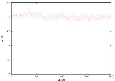
(c) LE for XOR

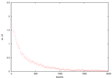
(d) LE for AND

Figure 3: Average STE and LE for XOR and AND for the two-layer network with 20 input neurons and without hidden layer. The STE graphs are clipped at 10 as this error is only exceeded for the first 20 epochs as discussed in the main text.

Table 1: Mean STE and LE averaged over epochs 900–999 and 1900-1999 and 100 networks for each condition. Most significant digit of error of the mean shown in ().

Operation	Error	900-999	1900-1999
AND	STE	3.37(2)	2.35(3)
	LE	0.170(3)	0.076(2)
J0	STE	3.84(2)	2.83(3)
	LE	0.230(4)	0.149(3)
TRUE	STE	3.32(2)	2.55(3)
	LE	0.161(3)	0.078(3)
XOR	STE	3.55(2)	3.08(3)
	LE	0.200(4)	0.157(2)

(a) 12 inputs, 20 hidden neurons

Operation	Error	900-999	1900-1999
AND	STE	1.98(1)	0.41(1)
	LE	0.104(2)	0.022(1)
J0	STE	1.29(1)	0.37(1)
	LE	0.047(2)	0.007(1)
TRUE	STE	0.570(9)	0.084(2)
	LE	0.010(1)	0
XOR	STE	6.39(1)	5.70(1)
	LE	2.012(8)	1.994(7)

(b) 20 inputs, no hidden layer

Operation	Error	900-999	1900-1999
AND	STE	6.26(2)	5.52(2)
	LE	0.75(5)	0.469(4)
J0	STE	6.03(2)	5.60(3)
	LE	0.612(5)	0.390(5)
TRUE	STE	6.34(2)	5.29(3)
	LE	0.641(6)	0.371(6)
XOR	STE	6.56(2)	5.978(3)
	LE	0.761(5)	0.518(5)

(c) Control case, 12 inputs, 12 hidden neurons

Operation	Error	900-999	1900-1999
AND	STE	6.69(1)	5.90(1)
	LE	0.843(5)	0.648(5)
J0	STE	4.70(1)	3.83(1)
	LE	0.377(4)	0.261(3)
TRUE	STE	5.35(1)	3.78(1)
	LE	0.453(4)	0.179(3)
XOR	STE	9.16(2)	8.88(1)
	LE	1.978(8)	1.968(7)

(d) Control Case: 12 inputs, no hidden layer

5.1 Discussion

Figures 2–3 present average learning curves for STE and LE for the two network configurations for logical operations XOR and AND averaged over 100 runs. Learning curves for J0 and TRUE are very similar to AND for each network and are therefore not shown.

The course for STE curves is similar for all cases: From about epoch 20 the STE errors are below 10 and decay first relatively steeply and then slower. However the STE for the three-layer networks starts with a low error value in the first epochs which rises steeply to very high values up to 400 and then rapidly decays to values below 10 in the first 20 epochs (not shown, STE graphs clipped at 10). The reason for the marked peak in three-layer networks only is that initial weights were chosen so that no output spikes are generated at all. As weights increase by scaling eq. 4 and as more output spikes are generated, the errors increase until most of them are removed again via eq. 2. For LE the picture is similar, however testing the interpretation of the output, LE starts always at the random level 2, perhaps slightly increasing beyond that around epoch 20 and then decreases to lower values (with the exception of XOR for the two-layer networks, see below). All in all, errors decrease in a way similar to many other supervised network learning algorithms.

The XOR problem in the three-layer network reaches level after about 1500 epochs and does not decay after that, see fig. 2(a), while the STE learning curve for XOR in the two-layer networks is still decreasing after 2000 epochs, see fig. 3(a). Additional simulations for up to 10000 epochs however confirmed that the STE reaches a minimum after about 3000 epochs for the two-layer networks, and that LE does not change at all, but fluctuates around the random performance value $2$ throughout all epochs.

It may be seen that all curves are very rough in nature and this is discussed below. Tables 1(a) and (b) summarise the simulation results in terms of STE and LE averaged over all 100 networks for a given configuration and the 100 epochs from 900–999 and 1900–1999 respectively.

The amount of activation that the output neuron can get from its predecessor layer is similar for the three (with 20 neurons in the hidden layer) and the two-layer networks (with 20 neurons in the input layer) and a comparison between them is interesting. We discuss the different logical operations at this point. The two-layer network is best except for the XOR operation, and its LE performance on XOR stays throughout training at a random level. In other words, the networks without hidden layer are not able to learn the XOR problem reliably.

The XOR operation reaches an LE value of between 0.157 and 0.200 for the three-layer networks. If we assume that networks with $\acs{LE}\neq 0$ have at most $\acs{LE}=1$, then this indicates that more than a fraction of $0.843=1-0.157$ of these networks produces no logical error on average for any epoch from 1900-1999. In other words, the three-layer networks can learn the XOR problem, although not with a reliability fit for technical purposes.

As to the other logical operations, TRUE and J0 do best in two layer networks. AND and XOR are the operations where information from the two inputs $J_{0}$ and $J_{1}$ needs to be combined, and they are learned with a somewhat higher STE and LE error rate. For the three-layer network, J0 is hardest to learn. With a large hidden layer that mixes spikes from both input banks it might be more difficult to find enough spikes that convey information about only one of the inputs banks.

Overall relative differences between logical operations are lower for the three-layer networks. Hence the difficulties to match a spike train outweigh the difficulty to perform the computation.

5.2 Error Roughness

Despite averaging over 100 networks, it is obvious that the learning curves are not as smooth as for rate neuron learning algorithms. This roughness stems from that of individual learning curves, see fig. 4 for a typical successful network trained on the XOR task. Individual networks occasionally lose a good solution and refind it later. This can lead to large changes in STE. However changes in LE might not be as pronounced as in STE, see fig. 4(c). These abrupt changes are an effect of the discontinuous nature of spike events, where relatively large discrete jumps in the errors for individual networks are expected when weights are slightly changed but an additional output spike is created or disappears.

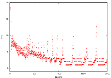
(a) STE for all epochs, clipped at 20.

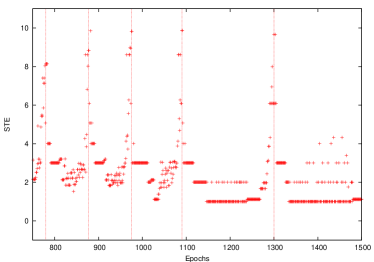
(b) STE. Enlargement of (a) for epochs 750–1500.

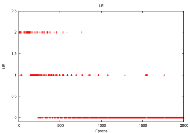
(c) LE for all epochs.

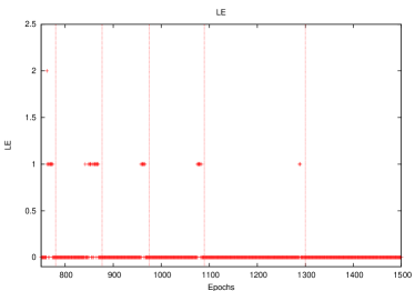
(d) LE. Enlargement of (c) for epochs 750–1500.

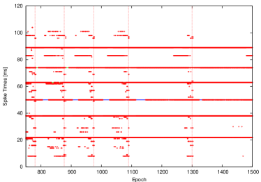
(e) Spike Trains for epochs 750–1500.

Figure 4: Typical individual learning curves and spike train evolution for a single network with 12 inputs and 20 hidden neurons trained on XOR. (a)/(c) The network is generally performing well from about 750 epochs, however it loses a solution that is close to the target spike trains for short times, indicated by the peaks of STE. However LE is less effected. (b)/(d) Enlargement of (a)/(c) for epochs 750–1500. Vertical dotted lines indicate the peaks of STE. LE deviates from 0 immediately before the STE peaks and then returns to 0. Towards the end of the cascade of peaks the networks settles into a closer approximation of the target spike trains with STE frequently at about $1.5$. (e) Spike times evolution for epochs 750–1500: The actual output spike times are represented as rings. Desired spike times are represented as the solid horizontal lines. These are covered heavily with actual spikes that hit the right spike time. This graph overlays actual and desired output spike times for all XOR input-output patterns 000,011,101,110. That all desired spikes time seem to be hit, does not imply that any single output train hits all target times. Vertical dotted lines again indicate the epochs with STE peaks. These are correlated with a reorganisation of spike time patterns.

5.3 Further Control Cases

We also ran two further network configurations as control cases, namely a three-layer network still with 12 inputs, but only 12 neurons in the hidden layer, and a two-layer network with only 12 inputs. Learning curves were qualitatively similar to the other networks, but performance (see table 1(c) and (d)) was worse than their counterparts with bigger hidden or input layer.

That the three-layer network with 20 hidden neurons and 12 inputs performs better on all logical operation than the two-layer network with 12 inputs, demonstrates that, as for rate neuron networks, a hidden layer is useful to preprocess and mix inputs even though the total information fed into the networks is the same.

6 Conclusion

The present simulations – to our knowledge for the first time – present an example of supervised learning in layered spiking neural networks where inputs and outputs are encoded as spike trains of multiple spikes. It extends and builds on other supervised learning algorithms for spiking neural networks like ReSuMe and SpikeProp. Restrictions on spike patterns in SpikeProp and its extensions (one latency-coded output spike) are more severe than in the present simulations (three timed output spikes). ReSuMe has only been used on either single neurons or on read-outs of LSM, nor has it been attempted to implement a simple but non-trivial computation like the XOR operation. SpikeProp suffers from silent neurons in the hidden layer for which no error signals can be obtained. We sidestep a similar problem by scaling weights multiplicatively so that firing rates are kept within a specified range.

Our results indicate that on average more than 80% of the three-layer networks in any one of the final 100 epochs compute the not linearly separable XOR operation correctly while two-layer networks do not. This extends a similar observation for layered networks of rate neurons [16]. However the roughness of the learning curves suggests that networks frequently lose and refind a good solution.

ReSuMe as applied to layered networks is certainly not reliable enough for technical purposes or even for information processing in the nervous system. However we have so far only considered a single output spike train. If a single neuron and its spike train are individually not reliable, they may be as an ensemble. It has been observed that neurons driven with the same inputs can be trained to produce different spike trains [11]. It is therefore possible that a bank of output neurons driven from the same hidden layer, but producing different spike trains for the same logical value, can be trained successfully, as incoming weights of the output neurons and their targets are independent. This ensemble would be more reliable to represent the true or false output than any neuron on its own [19]. Multiple output spike trains mirror using banks of inputs, too. In addition, this is also more realistic as in nature neurons act collectively to encode information and omission or addition of single spikes does not seem to be critical [6, 9].

While it is often clear that a given network structure is Turing-equivalent, it is less clear what computations can be learnt and how they are implemented on a given network in a natural way. There has been a successful stream of research to analyse what computational representations a rate network evolves for a given computational problem [2, 22, 8]. In this spirit, we believe it is now time to explore spiking neural networks and their computational capabilities.

Acknowledgements

The authors thank Yaochu Jin, Scott Notley and Susanne Schindler for comments on an earlier version of this article, and Susanne also for support with fig. 1. AG also personally thanks Susanne Schindler (and the AP) for her invaluable company without which this work would not have been.

AG’s part of the work was conducted under the Engineering and Physical Sciences Research Council (UK) grant EP/I014934/1.

References

- Bengio et al [1994] Bengio Y, Simard P, Frasconi P (1994) Learning long-term dependencies with gradient descent is difficult. IEEE Transactions on Neural Networks 5(2):157–166
- Bodén and Wiles [2000] Bodén M, Wiles J (2000) Context-free and context-sensitive dynamics in recurrent neural networks. Connection Science 12(3/4):197–210
- Bohte et al [2002] Bohte S, Kok J, Poutré HL (2002) Spike-prop: error-backpropagation in multi-layer networks of spiking neurons. Neurocomputing 48(1–4):17–37
- Booij and tat Nguyen [2005] Booij O, tat Nguyen H (2005) A gradient descent rule for spiking neurons emitting multiple spikes. Information Processing Letters 95:552–558
- Enderton [2001] Enderton H (2001) A mathematical introduction to logic, 2nd edn. Academic Press, Boston
- Gerstein and Kirkland [2001] Gerstein GL, Kirkland KL (2001) Neural assemblies: technical issues, analysis, and modeling. Neural Networks 14(6–7), DOI doi:10.1016/S0893-6080(01)00042-9
- Gerstner and Kistler [2002] Gerstner W, Kistler W (2002) Spiking Neuron Models: Single Neurons, Populations, Plasiticity. Cambrige University Press
- Grüning [2006] Grüning A (2006) Stack- and queue-like dynamics in recurrent neural networks. Connection Science 18(1):23–42.
- Izhikevich [2007] Izhikevich EM (2007) Solving the distal reward problem through linkage of STDP and Dopamine signalling. Cerebral Cortex 17:2443–2452, DOI 10.1093/cercor/bhl152
- Kasiński and Ponulak [2006] Kasiński A, Ponulak F (2006) Comparison of supervised learning methods for spike time coding in spiking neural networks. Int J Appl Math Comput Sci 16(1):101–113
- Kasiński and Ponulak [2005] Kasiński A, Ponulak P (2005) Experimental demonstration of learning properties of a new supervised learning method for the spiking neural networks. In: Proceedings of the 15th International Conference on Artificial Neural Networks: Biological Inspirations, Lecture Notes in Computer Sciences, vol 3696, pp 145–153
- Kistler and van Hemmen [2000] Kistler W, van Hemmen LJ (2000) Modeling synaptic plasticity in conjunction with the timing of pre- and postsynaptic action potentials. Neural Computation 12:385–405
- Legenstein et al [2005] Legenstein R, Naeger C, Maass W (2005) What can a neuron learn with spike-timing-dependent plasticity? Neural Computation 17(11):2337–2382
- Legenstein et al [2008] Legenstein R, Pecevski D, Maass W (2008) A learning theory for reward-modulated spike-timing-dependent plasticity with application to biofeedback. PLoS Computational Biology 3(10):1–27
- Maass et al [2002] Maass W, Natschläger T, Markram H (2002) Real-time computing without stable states: A new framework for neural computation based on perturbations. Neural Computation 14(11):2531–2560
- Minsky and Papert [1988] Minsky M, Papert S (1988) Perceptrons: an introduction to computational geometry, expanded edn. MIT Press, Cambridge, Mass., London
- Nemenman et al [2008] Nemenman I, Lewen GD, Bialek W, de Ruyter van Steveninck RR (2008) Neural coding of natural stimuli: Information at sub-millisecond resolution. PLOS Comp Biol 4(3)
- Okun and Lampl [2009] Okun M, Lampl I (2009) Balance of excitation and inhibition. Scholarpedia 4(8):7467, DOI 10.4249/scholarpedia.7467
- Polikar [2006] Polikar R (2006) Ensemble based systems in decision making. IEEE Circuits and Systems Mag 6(3):21–45
- Ponulak [2008] Ponulak F (2008) Analysis of the ReSuMe learning process for spiking neural networks. Int J Appl Math Comput Sci 18(2):117–127, DOI 10.2478/v10006-008-0011-1
- Ponulak and Kasiński [2010] Ponulak F, Kasiński A (2010) Supervised learning in spiking neural networks with ReSuMe: Sequence learning, classification and spike shifting. Neural Computation 22:467–510
- Rodriguez [2001] Rodriguez P (2001) Simple recurrent networks learn context-free and context-sensitive languages by counting. Neural Computation 13:2093–2118
- Rojas [1996] Rojas R (1996) Neural Networks – A Systematic Introduction. Springer, Berlin
- van Rossum [2001] van Rossum MCW (2001) A novel spike distance. Neural Computation 13:751–763
- Rumelhart et al [1986] Rumelhart D, Hinton G, Williams R (1986) Learning internal representations by error propagation. In: Rumelhart DE, McClelland JL, et al (eds) Parallel Distributed Processing – Explorations in the Microstructure of Cognition, vol 1 – Foundations, MIT Press, Cambridge, Mass., chap 8, pp 318–362
- Schrauwen and Campenhout [2004] Schrauwen B, Campenhout JV (2004) Extending SpikeProp. In: Proceedings of the International Joint Conference on Neural Networks (IJCNN), pp 471–476
- Shepard et al [2009] Shepard JD, Rumbaugh G, Wu J, Chowdhiry S, Plath N, Kuhl D, Huganir RL, Worley PF (2009) Arc mediates homoestatoc synaptic scaling of ampa receptors. Neuron 52(3):475–484
- Siegelmann and Sontag [1995] Siegelmann HT, Sontag ED (1995) On the computational power of neural nets. Journal of Computer and System Sciences 50:132–150
- Sporea and Grüning [2011] Sporea I, Grüning A (2011) Reference time in SpikeProp. In: Proceedings of the International Joint Conference on Neural Networks (IJCNN), IEEE, San Jose, CA.
- Tiňo and Mills [2006] Tiňo P, Mills AJ (2006) Learning beyond finite memory in recurrent networks of spiking neurons. Neural Computation 18(3):591–613