All Transients, All the Time:
Real-Time Radio Transient Detection with Interferometric Closure Quantities

Abstract

We demonstrate a new technique for detecting radio transients based on interferometric closure quantities. The technique uses the bispectrum, the product of visibilities around a closed-loop of baselines of an interferometer. The bispectrum is calibration independent, resistant to interference, and computationally efficient, so it can be built into correlators for real-time transient detection. Our technique could find celestial transients anywhere in the field of view and localize them to arcsecond precision. At the Karl G. Jansky Very Large Array (VLA), such a system would have a high survey speed and a 5$\sigma$ sensitivity of 38 mJy on 10 ms timescales with 1 GHz of bandwidth. The ability to localize dispersed millisecond pulses to arcsecond precision in large volumes of interferometer data has several unique science applications. Localizing individual pulses from Galactic pulsars will help find X-ray counterparts that define their physical properties, while finding host galaxies of extragalactic transients will measure the electron density of the intergalactic medium with a single dispersed pulse. Exoplanets and active stars have distinct millisecond variability that can be used to identify them and probe their magnetospheres. We use millisecond time scale visibilities from the Allen Telescope Array (ATA) and VLA to show that the bispectrum can detect dispersed pulses and reject local interference. The computational and data efficiency of the bispectrum will help find transients on a range of time scales with next-generation radio interferometers.

1. Introduction

Since the discovery of the first pulsar, radio observations have steadily revealed a wide range of fast ($\lesssim 1$s) transient phenomena. Pulsars (Hewish et al., 1968; Backer et al., 1982; Camilo et al., 2006), planets and active stars (Hallinan et al., 2007; Grießmeier et al., 2007), and peculiar new transients (McLaughlin et al., 2006; Lorimer et al., 2007) all have distinct radio phenomenology related to the physics of the host and the medium through which the signal propagates.

While large, single-dish telescopes have pioneered the study of fast radio transients, the nature of their design has several limits. Single-dish telescopes can only localize an individual pulse to somewhere in its field of view (typically arcminutes; Manchester et al., 2001). Timing of periodic emission can localize very precisely, but individual pulses can’t be localized well enough to easily identify optical or X-ray counterparts. Since interferometers simultaneously have a large collecting area and a large field of view, they survey more efficiently than single-dish telescopes. Survey speed scales roughly the square of the product of the number of dishes and their diameter; this predicts that the VLA surveys almost 40 times faster than the Green Bank Telescope, assuming all other factors are equal. Despite this potential, next-generation radio interferometers (VLA, PAPER, LOFAR, ASKAP, and MeerKAT) have fast transients observing modes that are essentially identical to the single-dish concept: point one or more beams on the sky and search for pulses (Macquart, 2011; Siemion et al., 2011).

In principle, interferometers have much more information available to them because they detect the electromagnetic wave over a distributed array of receivers. Instead of forming a beam, interferometers can measure visibilities by correlating signals across the array. Visibilities contain spatial information that can reject interference and localize a source to arcsecond precision over a large field of view. Traditionally, visibilities haven’t been used in this way because it was difficult to run correlators this fast and the data volume was too large to handle or efficiently search for pulses (Law et al., 2011). As a result, a standard radio interferometer averages data to second time scales, losing nearly all information about millisecond variability in the sky. Even on these longer time scales, imaging algorithms are complex and subject to subtle statistical biases (Condon et al., 1998). The challenge of data rates and volumes is expected to grow with next-generation interferometers, which will have more antennas, wider bandwidths, and larger fields of view (Perley et al., 2011).

Here, we present a technique that reduces the challenge of detecting transients in visibilities to the much simpler single-dish problem, while maintaining the utility of visibilities. The technique is based on the “bispectrum”, a quantity formed from visibilities that is sensitive to a point source anywhere in the field of view (Cornwell, 1987; Kulkarni, 1989; Rogers et al., 1995). Differencing visibilities makes it possible to interpret the bispectrum as a statistic for transients anywhere in the field of view on time scales from milliseconds to seconds. We describe an algorithm for real-time, arcsecond localization of transients using raw visibilities from a radio interferometer.

The theory of closure quantities and their application to transients is presented in §2. In §3 we test the theoretical predictions with millisecond time scale visibilities from the VLA and the “Pocket Correlator” (PoCo) instrument at the ATA (Law et al., 2011). As shown in §4, this technique has a moderate computational demand and can reduce the flow of data to a manageable size. We conclude with thoughts about new science accessible with this technique and how it can address the growing challenge of big data in the study of transients with radio interferometers.

2. Theory of Transient Detection with the Bispectrum

Closure quantities are the combination of visibilities from antennas that form a closed loop (Cornwell, 1987). An example of a closure quantity is the closure phase or triple phase, which is the sum of the visibility phase from three baselines, $\phi_{\rm{ijk}}=\phi_{ij}+\phi_{jk}+\phi_{ki}$. This combination is useful because it is independent of phase errors associated with any individual antenna. Closure quantities have largely been developed for very long baseline interferometry, because they make it possible to detect a source even if phase calibration is unstable (Rogers et al., 1995). An interesting corollary is that the triple phase responds in the same way to a point source anywhere in the field of view.

A related closure quantity is the product of visibilities on a closed loop, called the closure triple or bispectrum. The bispectrum can be written as $b_{ijk}=a_{ij}\,a_{jk}\,a_{ki}\,e^{i\phi_{\rm{ijk}}}$, where $a_{ij}$ are the amplitudes of visibilities for baseline $ij$. In the absence of signal, the bispectra have a mean at the origin of the real-imaginary plane with variance proportional to the cube of the thermal noise. A celestial point source is coherent across the array and moves all bispectra to positive real values proportional to the cube of its brightness (Kulkarni, 1989; Rogers et al., 1995). This makes the bispectrum useful for the statistical detection of a source anywhere in the field of view.

An interferometer can detect sources with a low signal to noise ratio (SNR) per baseline, $s$, by coherently combining signals over many baselines. For a homogeneous array of $n_{a}$ elements, there are $n_{bl}=n_{a}(n_{a}-1)/2$ independent baselines, so coherently combining all baselines improves SNR to $s\,\sqrt{n_{bl}}$. For combinations of three antennas, there are $n_{tr}=n_{a}(n_{a}-1)(n_{a}-2)/6$ closed possibilities. It can be shown that some triple phases are redundant (e.g., $\phi_{123}=\phi_{124}+\phi_{143}+\phi_{234}$), which leaves only $(n_{a}-1)\,(n_{a}-2)/2$ “unique” triples (Rogers et al., 1995). However, the bispectrum is subject to different correlated noise properties, since it is formed by multiplying complex visibilities rather than summing scalar phases. As a result, in the limit of small $s$, all $n_{tr}$ triples are independent (Kulkarni, 1989) and can be coherently combined to improve SNR.

Interferometers can detect a source in many ways. Coherent beamforming sums complex visibilities with weights to direct the beam . Antenna-based incoherent beamforming sums the power detected at each antenna, while baseline-based beamforming sums power detected on each baseline (i.e., the amplitude of a visibility; Thompson et al., 2001). In all of these cases, the SNR of a source detection can be written in terms of the SNR per baseline and size of the array (Kulkarni, 1989; Rogers et al., 1995). The SNR for coherent beamforming, bispectrum, antenna-based incoherent beamforming, and baseline-based incoherent beamforming are:

$$\rm{SNR}_{bfc} = s\,\sqrt{n_{bl}},$$

$$\rm{SNR}_{bisp} = \frac{1}{2}\,s^{3}\,\sqrt{n_{tr}},$$

$$\rm{SNR}_{bfia} = s\,\sqrt{n_{a}},\,$$

$$\rm{SNR}_{bfib} = \frac{1}{2}\,\frac{s^{2}}{\sqrt{1+s^{2}}}\,\sqrt{n_{bl}}$$ (1)

Note that for constant sources, the relation for SNR_bisp is only valid when $s$ is smaller than 1 (Kulkarni, 1989). However, for transient sources the noise is measured off pulse. This removes the correlated noise effect and makes the $s^{3}$ scaling valid for all $s$. We refer to these relations as the “apparent SNR”, since they are valid when the statistics are measured relative to the standard deviation off source. For Gaussian statistics, the apparent SNR is related to the false positive rate as $\frac{1}{2}*\left(1-\rm{erf}\left(\frac{SNR}{\sqrt{2}}\right)\right)$ (Rogers et al., 1995); a $5\sigma$ deviation corresponds to a false-positive rate of $2.87\times 10^{-7}$.

An important complication to this SNR analysis is that an individual bispectrum measurement is not Gaussian distributed. Visibilities are Gaussian distributed, so multiplying three, noise-like complex visibilities together produces a long-tailed distribution. The product of three independent real-valued random variables follows the Meier G function G${}^{3,0}_{0,3}$ (Lomnicki, 1967); we are not aware of an analytic expression for the real part of the product of three complex random variables. Regardless of the exact distribution, the Central Limit Theorem predicts that the mean of many, independent bispectra will approach a Gaussian distribution (Rogers et al., 1995). In the presence of pure noise, each bispectrum in an array is independent (Kulkarni, 1989), so the distribution of the mean bispectrum will approach a Gaussian as the number of elements in the array grows, as shown in Figure 1.

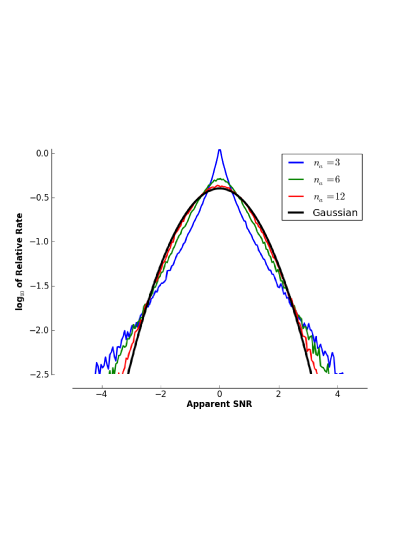
Figure 1.— Simulated histograms of the noise distribution of the real part of the mean bispectrum. Each bispectrum is calculated by multiplying random complex visibilities for an array of $n_{a}$ antennas producing $n_{bl}$ independent visibilities. The real and imaginary parts of the visibilities are sampled from a Gaussian with standard deviation of 1 and mean of 0. The mean bispectrum for $n_{a}=3$ (the smallest array with a bispectrum) is centrally peaked with long tails. For larger arrays, the distribution of the mean bispectrum narrows and approaches that of a Gaussian, as expected from the Central Limit Theorem. The distribution can also be used to estimate the false-positive rate for a signal of a given apparent SNR.

To include this effect in our sensitivity calculation, we simulated noise-like visibilities and directly measured the flux limit of the coherent beamforming and bispectrum statistics as a function of array size, $n_{a}$. The flux limit is quantified by calculating $s$ (from Equations 1) that would produce the simulated 5$\sigma$ false-positive rate under Gaussian statistics. This simulation shows that the flux limit of coherent beamforming matches the expectation for a Gaussian-distributed quantity. However, the mean bispectrum has a larger false-positive rate than expected for an apparent 5$\sigma$ deviation, especially for small $n_{a}$ where the Central Limit Theorem has less effect. We use these simulations to define an effective bispectrum 5$\sigma$ flux limit that produces the Gaussian false-positive rate. The effective 5$\sigma$ flux limit is higher than predicted by Gaussian statistics at a level of 53%, 26%, 13%, and 6% for $n_{a}=3,6,12,24$, respectively. For this work, we assume the mean bispectrum is Gaussian distributed, which is reasonable for arrays larger than a roughly a dozen elements for a 5$\sigma$ flux limit. Future work will develop a more general expression for the false-positive rate and optimizations for transient detection in the non-Gaussian domain.

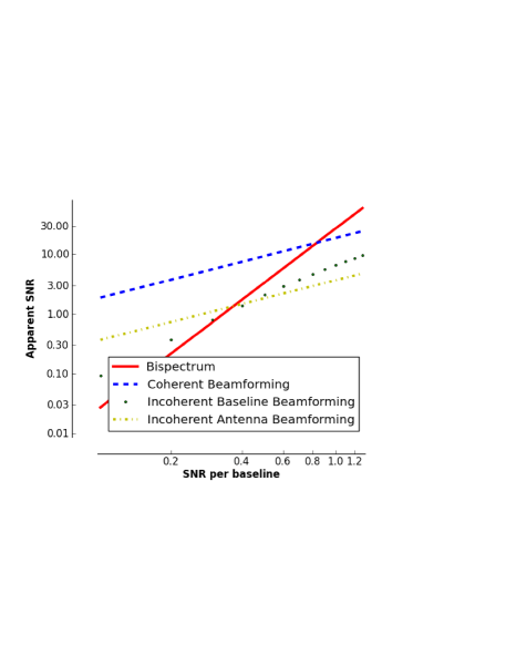
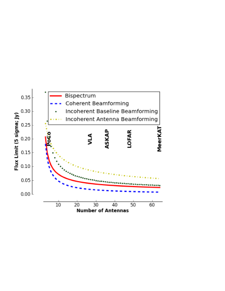
Figure 2.— Top: Apparent SNR for coherent beamforming, bispectrum, and incoherent beamforming techniques as a function of SNR per baseline for a 27-element array. For an effective SNR, defined according to the false-positive rate, the bispectrum SNR never exceeds that of coherent beamforming. Bottom: The effective 5$\sigma$ flux limits as a function of the number of antennas. The effective bispectrum flux limit includes a correction due to non-Gaussianity. The text marks the sizes of major new and planned observatories, including LOFAR (Stappers et al., 2011), MeerKAT (Booth et al., 2009), and ASKAP (Johnston et al., 2008). This assumes Stokes I detection with a SEFD of 400 Jy, 1 GHz bandwidth, and 10 ms integrations, which gives a 1$\sigma$ sensitivity of 63 mJy per baseline. For reference, the VLA 5$\sigma$ 10-ms sensitivity is 17 mJy for coherent beamforming, 38 mJy for the bispectrum, 50 mJy for baseline incoherent, and 85 mJy for antenna incoherent detection.

Figure 2 shows how the apparent SNR of four techniques scales with SNR per baseline for a 27-element array like the VLA. The apparent bispectrum SNR scales as $s^{3}$, giving it a strong response to bright sources and very little response to faint sources. However, the effective bispectrum SNR, defined according to a Gaussian false-positive rate, would be less sensitive for large $s$. Our simulations suggest that the effective bispectrum SNR never exceeds that of coherent beamforming.

The bottom panel of Figure 2 shows the effective 5$\sigma$ flux limit for an array with $n_{a}$ elements and sensitivity like the VLA. For the beamforming techniques, this plot essentially shows how the lines in the top panel intersect $\rm{SNR}=5$ as the array size changes. For the bispectrum, the effective flux limit is shown by correcting for sensitivity loss due to non-Gaussianity, as measured in our simulations. Generally, since large arrays are sensitive to pulses with SNR per baseline much less than one, coherent beamforming and imaging become more sensitive than the bispectrum as $n_{a}$ increases. For large $n_{a}$, the bispectrum and incoherent beamforming techniques scale similarly ($s\propto n_{a}^{-1/2}$), so the bispectrum is always more sensitive than the incoherent techniques.

To interpret the bispectrum as the brightness of a transient requires subtracting the signature of constant emission from the visibilities. Proper subtraction requires that the visibility fringe does not change over background subtraction time. The maximum fringe rate is equal to the product of the rate of change of the longest baseline in the (u,v) plane and the largest direction cosine. In units of radians per day, the maximum fringe rate is $\pi\,b_{\rm{max}}\,\theta_{\rm{f.o.v.}}/\lambda$, where $b_{\rm{max}}$ is the longest baseline, $\theta_{\rm{f.o.v.}}$ is the field of view in radians, and $\lambda$ is the wavelength. More precisely, the error from subtracting visibilities leaves residual errors proportional to the brightness of sources in the field. Thompson et al. (2001) quantify the effect of time smearing as a reduction in the peak brightness of a source. For small changes, we can parametrize this in terms of a 1.4 GHz VLA A configuration observation:

$$\frac{S^{p}_{o}-S^{p}}{S^{p}_{o}}=6\times 10^{-4}\left[\left(\frac{\tau}{1\rm{s}}\right)\,\left(\frac{\theta_{\rm{f.o.v}}}{0\hbox{$.\!\!^{\circ}$}5}\right)\,\left(\frac{b_{\rm{max}}}{36\rm{km}}\right)\right]^{2}$$ (2)

where $\tau$ is the integration time scale.

For visibility (or image) subtraction, the peak flux lost from time smearing is similar to the flux residual in the differenced data given by Equation 2. This error will contribute to the mean bispectrum in proportion to the fraction of all triples that contain the long baseline. A single antenna is part of $(n_{a}-1)\,(n_{a}-2)/2$ triples, so errors for a long baseline are suppressed by the fraction of triples with that baseline, or a factor of $3/n_{a}$. Table 1 gives the longest time scale for which the bispectrum technique can be used on several radio interferometers. The time scale shows when the systematic errors introduced by background subtraction biases the mean bispectrum more than its thermal noise (1$\sigma$). This shows that most interferometers are suitable for using the bispectrum technique to search for transients as long as 1 second. The VLBA is so extended that the fringe rate can only be subtracted on millisecond time scales.

The bispectrum also contains information about the spatial distribution of emission. For a point source with large $s$, the standard deviation of complex bispectra is $\sigma_{B}=\sqrt{3}\,s^{2}\,Q^{3}$, where $Q$ is the noise per baseline (Kulkarni, 1989). Note that the standard deviation of bispectra is subject to correlated noise, as opposed to the standard deviation of the mean bispectrum in time. In contrast with a celestial source, interference is often in the near-field or subject to multipath propagation, which produces a random triple phase and a larger variance between bispectra. Another way to think about this is that terrestrial interference can look like a spatially-extended transient. The variance between bispectra provides a simple way to quantify whether a transient is point-like, as expected.

3. Demonstration

To use the bispectrum for transient detection, we assume that the real part of the mean of all bispectra is related to the brightness of a single source in the field of view. To use the bispectrum to detect and localize pulses, we propose the following algorithm:

• Subtract the mean visibility in time: Differencing visibilities removes all constant emission over some time scale, $\tau$.

• Dedisperse visibilities: The frequency-dependent arrival time must be removed to maximize SNR per baseline before creating the bispectra.

• Calculate mean and standard deviation of bispectra: The mean of bispectra gives a single value related to the significance of the transient, while the standard deviation is related to its spatial structure. Both the mean and standard deviation have dimensions of DM and time, so they can be used to set thresholds just as for a single-dish transients search.

• Calibrate and image candidate pulses: Bispectra can be used to make an image, but calibrated visibilities are needed for an accurate localization (Schwab & Cotton, 1983). Visibilities need to be buffered long enough to capture the dispersive delay across the band. The pulse is then imaged in a separate process.

Figure 3 shows how the bispectrum and coherent beamforming techniques detect pulses in PoCo data toward B0329+54. For both techniques, the plot shows the apparent pulse SNR when the pulsar is at the phase center, away from the phase center, and at the phase center but uncalibrated. The beamforming technique only detects the pulse when it is at the phase center and data are calibrated. The bispectrum detects the pulse regardless of its location or the phase calibration.

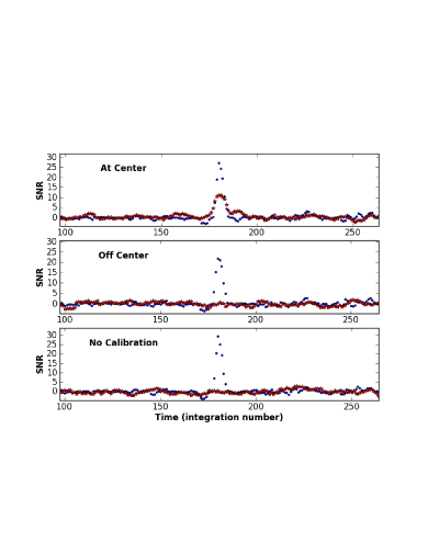
Figure 3.— Top: Time series of the apparent SNR measured by the bispectrum (blue) and with coherent beamforming (red) in 5-antenna PoCo data of pulsar B0329+54. The PoCo data have a time resolution of 1.2 ms and have been dedispersed assuming the known DM of B0329+54. This panel shows calibrated data with B0329+54 at the phase center. Middle: The same plot but with the pulsar off the phase center. Bottom: The same plot but with no phase calibration.

The apparent SNR of the bispectrum and coherent beamforming techniques for data including several pulses are shown in Figure 4. The top panel in Figure 4 shows that the PoCo pulse SNR distribution measured with beamforming and the bispectrum follow the relation of Rogers et al. (1995) well. Since there are only nine baselines and five triples in this analysis, the pulses shown here have relatively high $s$. The brightest pulse in this data has $s\sim 3$, corresponding to a brightness of about 50 Jy. A similar search with a larger array would have a much slower rise in $\rm{SNR}_{bisp}$ relative to $\rm{SNR}_{bfc}$.

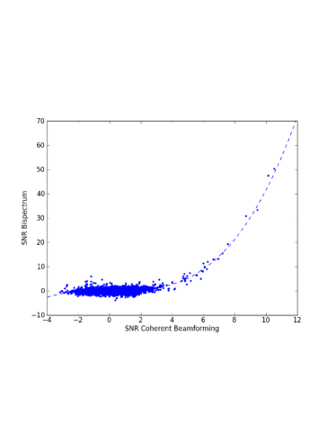
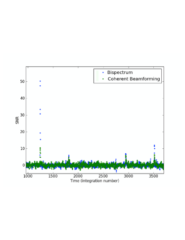
Figure 4.— Top: Apparent SNR of the bispectrum versus that of coherently beamforming of PoCo data toward B0329+54. The SNR is shown for each integration, regardless of significance. The dashed line shows the expected cubic dependence in the apparent SNR, as described in §2 and shown in Rogers et al. (1995). Bottom: A time series of the same two statistics for the same data. The rotation period of B0329+54 is about 600 integrations and four of the five pulses in this window are detected. For all detected pulses, the apparent bispectrum SNR is higher than that of beamforming, as expected for a small array as PoCo was used at the ATA.

Figure 5 shows how the bispectrum can distinguish between a celestial point transient and terrestrial interference. The top panel shows a typical dynamic spectrum for a VLA observation of the Crab pulsar with 12 millisecond integrations. As is well known from single-dish observing, interference is bright enough to be detected even after dedispersion. The bottom panel shows the mean bispectrum and standard deviation over bispectra for the same pulse and interference. The interference has a large standard deviation of bispectra, while the true Crab pulse follows the expected theoretical relation for $s\gg 1$.

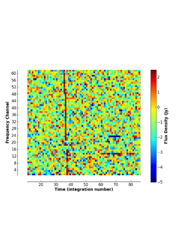
Figure 5.— Top: VLA dynamic spectrum toward the Crab pulsar at 1.4 GHz with 12 ms integrations and 128 MHz bandwidth. The dynamic spectrum is formed from the sum of all cross correlations, effectively forming a synthesized beam at the location of the Crab pulsar with a brightness in units of Janskys. At the left is a pulse from the Crab pulsar, which appears as a red vertical line with a slight kink due to dispersion. Two channels show interference of similar strength toward the right. Bottom: The apparent bispectrum SNR versus standard deviation of all bispectra for each dedispersed integration. The blue dashed line shows the theoretical expectation for a point source with $s\gg 1$. The one point near that line corresponds to the Crab pulse with $s\approx 4$.

4. Data and Operations Rates

Another strength of the bispectrum technique is its computationally efficiency. Table 2 shows how the computational demand scales for three coherent fast transient detection techniques at the VLA. These computational demand values are scaled to operations per second (flops) by multiplying by the integration rate in Hz. For the bispectrum and imaging techniques, the visibilities are dedispersed for each baseline and DM trial, while coherent beamforming is traditionally done before dedispersion. The imaging FFT requires $N_{\rm{bl}}\,N_{\rm{ch}}+5\,N_{\rm{pix}}^{2}\,\rm{log}_{2}N_{\rm{pix}}^{2}$ operations per image (Briggs et al., 1999). For the VLA D configuration, images require roughly 128 pixels per side, so $N_{\rm{pix}}=128$.

The bispectrum technique is the most computationally efficient technique for coherent pulse detection. Running this algorithm on 10 ms integrations at the VLA would require roughly 34 Gflops. Imaging is at least two times more demanding (this estimate excludes image cleaning). The coherent beamforming is driven by the number of beams needed to fill the field of view. Even in the compact D configuration, roughly 7000 beams are needed. The VLA A configuration would require about 900 times more synthesized beams and 3 Pflops to calculate. The large computational demand of coherent beamforming explains why it is typically only done with a few beams (Stappers et al., 2011).

Our pulse detection algorithm consists of many independent processes (across frequency, DM trial, and time), so the problem is readily parallelized. Moreover, aspects of the algorithm, such as the large number of multiplications and dedispersion, are well suited to GPUs (Magro et al., 2011; Clark et al., 2011). Table 2 suggests that the bispectrum computational demand can be met with a single GPU-accelerated server. However, the data rate associated with millisecond integrations from a large array can limit its application for some correlator designs, so careful attention must be paid to data rate bottlenecks. For example, at the VLA, the visibility integration time must be greater than roughly 10 ms, since nodes of the WIDAR compute cluster have 1 GbE input ports (Perley et al., 2011). A correlator that can produce visibilities at high ($\geq 10$ Gb s^-1) data rates is more likely to be limited by computational resources, driven largely by the need to dedisperse visibilities from each baseline. In this case, it will be easier to run this algorithm in real time on arrays with a small number of elements.

This description has focused on how the bispectrum can detect an astrophysical transient, but it can’t be used to localize it. While the bispectrum can be used to make images of the sky (Schwab & Cotton, 1983), precise localization requires external phase calibration. Thus, the final step in this algorithm is to save candidate transient data for calibration and imaging using traditional techniques (Briggs et al., 1999). This kind of post-processing is computationally more intensive than the bispectrum and is not feasible in real time on every integration. However, since we only need to calibrate and image the occasional candidate event, the total computational demand will still be dominated by the steps before the event detection.

5. Conclusion

We demonstrate how to use the bispectrum to detect and localize transients with radio interferometers. The technique produces a single statistic proportional to the brightness of celestial transients, thus reducing the problem of interferometric pulse detection to that of single-dish pulse detection. For a small cost in sensitivity, this technique makes an interferometer into a massive multibeam receiver with a proportionately large survey speed. Using coherent beamforming to survey a similar area with next-generation radio interferometers would require $10^{2}$ to $10^{5}$ times more computational power.

The bispectrum technique is efficient enough to build into a correlator for real-time, millisecond transient detection. This system could save visibility data associated with a candidate and apply standard calibration and imaging techniques to localize it to arcsecond precision. The growing capacity of correlators for interferometers will make it possible to run such a system in real time to commensally search all data for transients. The technique can also be used to find transients offline and on longer time scales. In that case, the bispectrum is useful because it is computationally simple, resistant to interference, and requires no calibration.

A real-time, commensal system would probe an unprecedented volume of data, giving it sensitivity to rare transients. Each pulse could be localized in real time to arcsecond precision, opening a range of new science. Pulses from rotating radio transients (McLaughlin et al., 2006) could be associated with X-ray counterparts to help address their relation to the normal pulsar population. The dispersion of extragalactic transients would measure the electron density of the intergalactic medium for the first time (McLaughlin & Cordes, 2003; Lorimer et al., 2007); localization will help find optical counterparts and redshifts to host galaxies for each pulse. A fast transients survey of the Galactic center could detect individual pulses from pulsars that would probe the dispersion toward the region and potentially find a pulsar in orbit around a supermassive black hole (Pfahl & Loeb, 2004; Macquart et al., 2010; Wharton et al., 2011). Magnetospheres of exoplanets and active stars can emit bright, complex bursts that could uniquely identify them (Lazio et al., 2004; Hallinan et al., 2006).

The strength of the bispectrum technique is its real-time ability to find transients throughout the field of view and reduce the flow of data to select times. This shows how algorithms will be key to efficiently extracting the best science in the era of big data. The ability to find pulses with interferometers may have application to communications problems, such as developing smart antennas for the efficient use of spectrum. If so, this technique would follow in the footsteps of previous transients searches that contributed to the development of Wi-Fi (Osullivan et al., 1978).

Table 1Time Scale for Using Bispectrum Technique on Radio Interferometers

Telescope	$\theta_{\rm{f.o.v.}}$	$b_{\rm{max}}$	Error	$\tau_{\rm{max}}$
	(deg)	(km)	(mJy)	(s)
VLA-A	0.5	36	5	0.2
VLA-D	0.5	1	5	7.2
VLBA	0.5	8611	70	0.003
PAPER	40	0.3	215	1.6
LOFAR	2.4	1	40	2
MeerKAT	1	20	7	0.2
ASKAP	3	2	18	1

Table 2Computational Demand per Integration for VLA Fast Transient Search Algorithms

Process	Bispectrum		Coherent Beamforming		Imaging
	Scaling	Demand	Scaling	Demand	Scaling	Demand
Subtraction	$10N_{\rm{bl}}N_{\rm{pol}}N_{\rm{ch}}N_{\rm{t}}$	14 Mop	$10N_{\rm{bl}}N_{\rm{pol}}N_{\rm{ch}}N_{\rm{t}}$	14 Mop	$10N_{\rm{bl}}N_{\rm{pol}}N_{\rm{ch}}N_{\rm{t}}$	14 Mop
Beamform	–	–	$3N_{\rm{b}}N_{\rm{bl}}N_{\rm{pol}}N_{\rm{ch}}N_{\rm{t}}$	28 Gop	–	–
Dedisperse	$N_{\rm{bl}}N_{\rm{pol}}N_{\rm{ch}}N_{\rm{DM}}N_{\rm{t}}$	287 Mop	$N_{\rm{b}}N_{\rm{ch}}N_{\rm{DM}}N_{\rm{t}}$	2.8 Gop	$N_{\rm{bl}}N_{\rm{pol}}N_{\rm{ch}}N_{\rm{DM}}N_{\rm{t}}$	287 Mop
Image	–	–	–	–	$1.5e6N_{\rm{DM}}N_{\rm{t}}$	602 Mop
Bispectrum	16 $N_{\rm{tr}}N_{\rm{pol}}N_{\rm{DM}}N_{\rm{t}}$	37 Mop	–	–	–	–
Total		339 Mop		33 Gop		904 Mop

References

- Baars et al. (1977) Baars, J. W. M., Genzel, R., Pauliny-Toth, I. I. K., & Witzel, A. 1977, A&A, 61, 99
- Backer et al. (1982) Backer, D. C., Kulkarni, S. R., Heiles, C., Davis, M. M., & Goss, W. M. 1982, Nature, 300, 615
- Booth et al. (2009) Booth, R. S., de Blok, W. J. G., Jonas, J. L., & Fanaroff, B. 2009, arXiv:0910.2935
- Briggs et al. (1999) Briggs, D. S., Schwab, F. R., & Sramek, R. A. 1999, Synthesis Imaging in Radio Astronomy II, 180, 127
- Camilo et al. (2006) Camilo, F., Ransom, S. M., Halpern, J. P., et al. 2006, Nature, 442, 892
- Clark et al. (2011) Clark, M. A., La Plante, P. C., & Greenhill, L. J. 2011, arXiv:1107.4264
- Condon et al. (1998) Condon, J. J., Cotton, W. D, Greisen, E. W., Yin, Q. F., Perley, R. A., Taylor¡ G. B., & Broderick, J. J. 1998, AJ, 115, 1693
- Cornwell (1987) Cornwell, T. J. 1987, A&A, 180, 269
- Deller et al. (2011) Deller, A. T., Brisken, W. F., Phillips, C. J., et al. 2011, PASP, 123, 275
- Grießmeier et al. (2007) Grießmeier, J.-M., Zarka, P., & Spreeuw, H. 2007, A&A, 475, 359
- Hallinan et al. (2006) Hallinan, G., Antonova, A., Doyle, J. G., et al. 2006, ApJ, 653, 690
- Hallinan et al. (2007) Hallinan, G., Bourke, S., Lane, C., et al. 2007, ApJ, 663, L25
- Hewish et al. (1968) Hewish, A., Bell, S. J., Pilkington, J. D. H., Scott, P. F., & Collins, R. A. 1968, Nature, 217, 709
- Johnston et al. (2008) Johnston, S., Taylor, R., Bailes, M., et al. 2008, Experimental Astronomy, 22, 151
- Kulkarni (1989) Kulkarni, S. R. 1989, AJ, 98, 1112
- Law et al. (2011) Law, C. J., Jones, G., Backer, D. C., et al. 2011, ApJ, 742, 12
- Lazio et al. (2004) Lazio, T. J., W., Farrell, W. M., Dietrick, J., et al. 2004, ApJ, 612, 511
- Lomnicki (1967) Lomnicki, Z. A. 1967, JRSS Series B, 29, 513
- Lorimer et al. (2007) Lorimer, D. R., Bailes, M., McLaughlin, M. A., Narkevic, D. J., & Crawford, F. 2007, Science, 318, 777
- Macquart (2011) Macquart, J.-P. 2011, ApJ, 734, 20
- Macquart et al. (2010) Macquart, J.-P., Kanekar, N., Frail, D. A., & Ransom, S. M. 2010, ApJ, 715, 939
- Magro et al. (2011) Magro, A., Karastergiou, A., Salvini, S., et al. 2011, MNRAS, 417, 2642
- Manchester et al. (2001) Manchester, R. N., Lyne, A. G., Camilo, F., et al. 2001, MNRAS, 328, 17
- McLaughlin & Cordes (2003) McLaughlin, M. A., & Cordes, J. M. 2003, ApJ, 596, 982
- McLaughlin et al. (2006) McLaughlin, M. A., Lyne, A. G., Lorimer, D. R., et al. 2006, Nature, 439, 817
- Osullivan et al. (1978) Osullivan, J. D., Ekers, R. D., & Shaver, P. A. 1978, Nature, 276, 590
- Parsons et al. (2010) Parsons, A. R., Backer, D. C., Foster, G. S., et al. 2010, AJ, 139, 1468
- Perley et al. (2011) Perley, R. A., Chandler, C. J., Butler, B. J., & Wrobel, J. M. 2011, ApJ, 739, L1
- Pfahl & Loeb (2004) Pfahl, E., & Loeb, A. 2004, ApJ, 615, 253
- Rogers et al. (1995) Rogers, A. E. E., Doeleman, S. S., & Moran, J. M. 1995, AJ, 109, 1391
- Schwab & Cotton (1983) Schwab, F. R., & Cotton, W. D. 1983, AJ, 88, 688
- Siemion et al. (2011) Siemion, A. P. V., Bower, G. C., Foster, G., et al. 2011, arXiv:1109.2659
- Stappers et al. (2011) Stappers, B. W., Hessels, J. W. T., Alexov, A., et al. 2011, A&A, 530, A80
- Thompson et al. (2001) Thompson, A. R., Moran, J. M., & Swenson, G. W., Jr. 2001, “Interferometry and synthesis in radio astronomy” by A. Richard Thompson, James M. Moran, and George W. Swenson, Jr. 2nd ed. New York : Wiley
- Wharton et al. (2011) Wharton, R. S., Chatterjee, S., Cordes, J. M., Deneva, J. S., & Lazio, T. J. W. 2011, arXiv:1111.4216