Present Bounds on New Neutral Vector Resonances from Electroweak Gauge Boson Pair Production at the LHC

Abstract

Several extensions of the Standard Model predict the existence of new neutral spin–1 resonances associated to the electroweak symmetry breaking sector. Using the data from ATLAS (with integrated luminosity of $\mathcal{L}=1.02\ \mbox{fb}^{-1}$) and CMS (with integrated luminosity of $\mathcal{L}=1.55\ \mbox{fb}^{-1}$) on the production of $W^{+}W^{-}$ pairs through the process $pp\to\ell^{+}\ell^{\prime-}\,/\!\!\!\!E_{T}$, we place model independent bounds on these new vector resonances masses, couplings and widths. Our analyses show that the present data excludes new neutral vector resonances with masses up to 1–2.3 TeV depending on their couplings and widths. We also demonstrate how to extend our analysis framework to different models working a specific example.

I Introduction

One of the primary physics goals of the CERN Large Hadron Collider (LHC) is the direct study of the electroweak symmetry breaking (EWSB) sector via the production of new states associated to it. The analyses of unitarity in the weak gauge boson scattering $W^{+}_{L}W^{-}_{L}\to W^{+}_{L}W^{-}_{L}$ indicates that there must be a contribution of the EWSB at the TeV scale Lee:1977eg , well within the LHC reach. There is a plethora of possibilities for the EWSB sector that contains new scalar and vector resonances, and the Standard Model (SM) represents only the minimal scenario, with a Higgs sector with one scalar Higgs boson being responsible for cutting off the growth of the weak gauge boson scattering amplitudes.

New vector resonances are a common feature of models where the EWSB is due to a new strongly interacting sector TC . Although the precision electroweak measurements and flavor changing neutral currents present an obstacle for strongly interacting theories, recent theoretical advances made possible the construction of models in agreement with the experimental constraints NTC . Furthermore, new spin–1 states are also present in extra dimension scenarios, in particular in Higgsless models hless where unitarity restoration takes place through the exchange of an infinite tower of spin–1 Kaluza-Klein excitations of the known electroweak gauge bosons Csaki:2003dt . Such scenarios can be viewed as the holographic version of strongly coupled theories ads-cft .

In this work, we derive bounds on new neutral spin–1 resonances ($Z^{\prime}$) associated to the EWSB from the available ATLAS and CMS data on $W^{+}W^{-}$ pair production

$$pp\to Z^{\prime}\to W^{+}W^{-}\to\ell^{+}\ell^{\prime-}\,/\!\!\!\!E_{T}$$ (1)

where $\ell$ and $\ell^{\prime}$ stand for electrons and muons. We perform a model independent analysis proposed in Refs. Alves:2009aa ; Eboli:2011bq . We present our results as constraints on the relevant spin-1 boson effective couplings, mass and width. For instance, our results indicate that $Z^{\prime}$’s coupling with SM strength to light quarks and to pairs $W^{+}W^{-}$ saturating the partial wave amplitudes can be excluded at 95% CL if their masses are lighter than $\simeq 1750$ GeV.

This paper is organized as follows. In Section II we present our model independent parameterization of the $Z^{\prime}$ properties. Section III contains a detailed accounting of the procedures used in our analyses. Our model independent results are presented in Section IV while we show in Section V that our analysis framework can be adapted to a specific model. Our conclusions are drawn in Section VI.

II Parameterization of the $Z^{\prime}$ properties

In order to evaluate the $Z^{\prime}$ production cross section via the channel (1) we must know the $Z^{\prime}$ couplings to light quarks and $W^{+}W^{-}$ pairs in addition to its mass and width. We do not assume any relation between these parameters (although they might be connected in a complete theory). Nevertheless, inspired by models where the new vector states interact with the light quarks and electroweak gauge boson via their mixing with the SM vectors, we assume that the $Z^{\prime}$ couplings exhibit the same Lorentz structure as those of the SM.

We normalize the $Z^{\prime}W^{+}W^{-}$ coupling by the value ${g_{Z^{\prime}WW}}_{max}$ that saturates the partial wave amplitude for the process $W^{+}W^{-}\to W^{+}W^{-}$ by the exchange of a $Z^{\prime}$,  Birkedal:2004au , i.e.

$${g_{Z^{\prime}WW}}_{max}=g_{ZWW}\,\frac{M_{Z}}{\sqrt{3}M_{Z^{\prime}}}$$ (2)

where $g_{ZWW}=g\leavevmode\nobreak\ c_{W}$ is the strength of the SM triple gauge boson coupling. Here $g$ stands for the $SU(2)_{L}$ coupling constant and $c_{W}$ is the cosine of the weak mixing angle.

We treat the $Z^{\prime}$ width as a free parameter since it can receive contributions from particles that do not play a role in our study, such as $b$ and $t$ quarks. The only bound to the $Z^{\prime}$ width is that it should be compatible with its couplings to light quarks and $WW$ pairs that is expressed by the lower bound  Alves:2009aa

$$\Gamma_{Z^{\prime}}\;>\;0.27\,|G|\,\,\left(\frac{M_{Z^{\prime}}}{M_{Z}}\right)^{2}{\rm GeV}\;,$$ (3)

where we have defined the combination

$$G=\left(\frac{g_{Z^{\prime}q\bar{q}}}{g_{Zq\bar{q}}}\right)\,\left(\frac{g_{Z^{\prime}WW}}{{g_{Z^{\prime}WW}}_{max}}\right)\,,$$ (4)

with $g_{Z^{\prime}q\bar{q}}$ being the $Z^{\prime}$ coupling to light quark pairs and $g_{Zq\bar{q}}=g/c_{W}$.

Within our approach we can express the cross section for the process (1) as

$$\sigma_{\rm tot}=\sigma_{\rm SM}\,+\,G\,\sigma_{\rm int}(M_{Z^{\prime}},\Gamma_{Z^{\prime}})\,+\,G^{2}\,\sigma_{Z^{\prime}}(M_{Z^{\prime}},\Gamma_{Z^{\prime}})$$ (5)

where the Standard Model, interference and new resonance contributions are labeled SM, int and $Z^{\prime}$ respectively.

III Analyses framework

ATLAS ATLASww and CMS CMSww analyzed the $W^{+}W^{-}$ production through the final state given in Eq. (1). Our strategy is to use the SM backgrounds that have been carefully evaluated by the experimental collaborations and we simulate only the $Z^{\prime}$ signal. However, in order to tune and validate our Monte Carlo we also simulated the SM production of $W^{+}W^{-}$ pairs and compared with the results presented by ATLAS and CMS.

We evaluated the signal and SM $W^{+}W^{-}$ cross sections by two different methods. In the first one, we used the package MADEVENT madevent to evaluate the ${\cal O}(\alpha^{4})$ signal matrix elements for the subprocesses $q\bar{q}\to\ell^{+}\nu\ell^{\prime-}\nu^{\prime}$, with $\ell/\ell^{\prime}=e,\mu$ as well as the small contribution with $\ell/\ell^{\prime}=\tau$ which then decays leptonically into either $e$ or $\mu$ and the corresponding neutrinos. Its output is fed into PYTHIA Sjostrand:2006za for parton shower and hadronization and a simple detector simulation provided by PGS 4 pgs4 . In what follows we will label it as “ME+Pythia+PGS-MC”. A second evaluation was made with a homemade Monte Carlo that evaluates the process (1) at parton level using the ${\cal O}(\alpha^{4})$ signal matrix elements for the subprocesses $q\bar{q}\to\ell^{+}\nu\ell^{\prime-}\nu^{\prime}$, with $\ell/\ell^{\prime}=e,\mu$. The scattering amplitudes for the relevant subprocesses were obtained using the package MADGRAPH madevent . In what follows we will label this calculation as “OUR ME-MC”. In both cases we used CTEQ6L parton distribution functions CTEQ6 and the MADEVENT default renormalization and factorization scales.

ATLAS analysis

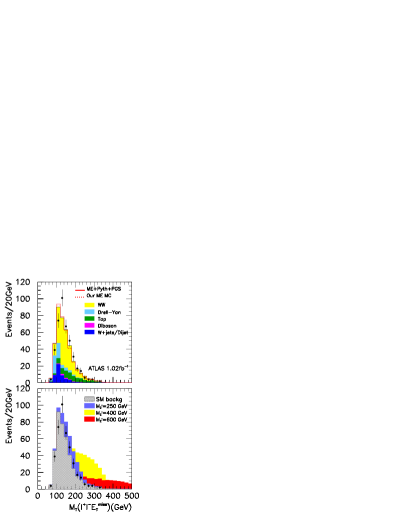
Figure 1: Upper panel: Transverse mass distribution of the SM contributions to the process $pp\to\ell^{+}\ell^{\prime-}/\!\!\!\!E_{T}$ calculated by ATLAS (colored histograms) together with the number of observed events by ATLAS (points with error bars) and the performance of ME+Pythia+PGS-MC (red solid) and OUR ME-MC (red dotted). The results shown correspond to an integrated luminosity of $\mathcal{L}=1.02\ \mbox{fb}^{-1}$.
Lower panel: Transverse mass distribution of the total SM contribution to the process $pp\to\ell^{+}\ell^{\prime-}/\!\!\!\!E_{T}$ (gray hashed) together with the total expected number of events including a $Z^{\prime}$ of 250 GeV with $G=0.5$ (blue), a $Z^{\prime}$ of 400 GeV with $G=1$ (yellow) and a $Z^{\prime}$ of 600 GeV with $G=1$ (red). For the three masses $\Gamma_{Z^{\prime}}=0.06M_{Z^{\prime}}$. We include also the ATLAS observed spectrum.

The ATLAS simulation of the $W^{+}W^{-}$ process was carried out at NLO and with an accurate detector simulation. In order to take into account some of these features included in the ATLAS evaluation of the SM $W^{+}W^{-}$ production we normalize our total cross section for the $ee$, $e\mu$ and $\mu\mu$ channels by an overall factor such that our two simulations yield the result presented in Table 2 of Ref. ATLASww after the same cuts have been implemented. In particular electrons and muons are accepted if

$$|\eta_{e}|<1.37\hbox{\ or\ }1.52<|\eta_{e}|<2.47\hbox{\ and\ }|\eta_{\mu}|<2.4.$$ (6)

Also, the lepton isolation requirement in ME+Pythia+PGS-MC simulation is that the sum of the energy in the calorimeter cells within a cone $\Delta R<0.3$ around the electron must be less than 4 GeV while in a cone $\Delta R<0.2$ around the muon, the sum $p_{T}$ of all other tracks is less than 10% of the $p_{T}$ of the muon. To implement this requirement in OUR ME-MC we simply impose:

$$\Delta R_{ee}>0.3\hbox{\ and\ }\Delta R_{e\mu,\mu\mu}>0.2\;.$$ (7)

Events are selected if they verify that the leading electron in the $e^{+}e^{-}$ channel and the electron in the $e\mu$ channel accomplish:

$$p_{T}>25\hbox{ GeV,}$$ (8)

while for the muons and the subleading electron in the $e^{+}e^{-}$ channel

$$p_{T}>20\hbox{ GeV.}$$ (9)

Furthermore,

$$M_{\ell\ell}>15\hbox{ GeV }\;\;,\;\;M_{e\mu}>10\hbox{ GeV},$$

$$|M_{\ell\ell}-M_{Z}|>15\hbox{ GeV, }$$ (10)

$$E_{T,\leavevmode\nobreak\ rel}^{miss}(ee)>40\hbox{ GeV }\;\;,\;\;E_{T,\leavevmode\nobreak\ rel}^{miss}(\mu\mu)>45\hbox{ GeV }$$

$$\hbox{and }E_{T,\leavevmode\nobreak\ rel}^{miss}(e\mu)>25\hbox{ GeV },$$

where $M_{\ell\ell}$ stands for the invariant mass of the lepton pair and the relative missing energy is defined as:

$$E_{T,\leavevmode\nobreak\ rel}^{miss}=\left\{\begin{array}[]{clc}&E_{T}^{miss}\times\sin{\Delta\phi_{\ell,j}}&\hbox{if}\ \ \Delta\phi_{\ell,j}<\pi/2\\ &E_{T}^{miss}&\hbox{if}\ \ \Delta\phi_{\ell,j}>\pi/2\end{array}\right.$$ (11)

with $\Delta\phi_{\ell,j}$ being the difference in the azimuthal angle $\phi$ between the transverse missing energy and the nearest lepton or jet.

Finally in ME+Pythia+PGS-MC simulation jets are reconstructed with the anti-$k_{T}$ algorithm arXiv:0802.1189 with a jet resolution parameter $\Delta R=0.4$ and we veto events containing jets with

$$p_{T}>30\hbox{ GeV and }|\eta_{j}|<4.5\;.$$ (12)

We present in Table 1 the overall normalization needed to tune our simulations to the ATLAS one. We have also verified that the relative event reduction due to each cut (8)–(10) in our simulations is in agreement to that reported in Table 2 of Ref. ATLASww .

Experiment	Monte Carlo	$ee$	$e\mu$	$\mu\mu$
ATLAS	OUR ME-MC	0.54	0.78	1.04
ATLAS	ME+Pythia+PGS-MC	0.66	0.95	1.2
CMS	OUR ME-MC	0.50	0.73	0.84
CMS	ME+Pythia+PGS-MC	0.60	0.91	1.08

Table 1: Overall multiplicative factors used to tune our Monte Carlos to the total number of events in the different flavour channels predicted by the ATLAS and CMS simulations.

In order to validate our Monte Carlo simulations for the SM $W^{+}W^{-}$ production we compare them with the ATLAS prediction for the transverse mass ($M_{T}$) spectrum after cuts in the top panel of Fig. 1. The results shown corresponds to an integrated luminosity of $\mathcal{L}=1.02\ \mbox{fb}^{-1}$. In this figure we evaluated just the SM $W^{+}W^{-}$ production and added the ATLAS results for the backgrounds. As we can see, both ME+Pythia+PGS-MC and OUR ME-MC simulations approximate very well the ATLAS results. However, it should be noticed that the three simulations, the one by ATLAS and two by us, present some discrepancy with the data at small transverse masses.

In the simulation of the $Z^{\prime}$ signal we employed the same normalization factors obtained from the $W^{+}W^{-}$ SM production for the channels $ee$, $e\mu$, and $\mu\mu$; see Table 1. Moreover, since our two simulations present a similar performance we adopted OUR ME-MC for our signal calculations because it is much faster. However we also verified that the results obtained are in agreement with those from ME+Pythia+PGS-MC for a few points of the parameter space.

We present, as an illustration, in the lower panel of Figure  1 the expected $M_{T}$ distribution for three different $Z^{\prime}$ masses for an integrated luminosity of 1.02 fb^-1, as reported by ATLAS, and after applying the cuts (6)–(12). The existence of this neutral vector resonance is characterized by an excess of events at higher $M_{T}$ values with respect to the SM expectations.

Consequently one can use the transverse mass spectrum to place constraints on the $Z^{\prime}$ properties. In order to do so we have constructed a binned log-likelihood function based on the contents of the different bins in the transverse mass distribution, i.e., the observed number of events $N_{d}^{i}$, and the expected events in the SM, $N_{B}^{i}$, plus the expected number of events in the presence of the $Z^{\prime}$, $N^{i}_{S}$, after applying the cuts (6)–(12). Assuming independent Poisson distributed $N_{d}^{i}$ it reads:

$$-2\ln L_{\rm ATLAS}(M_{Z^{\prime}},G,\Gamma_{Z^{\prime}})=$$

$$\begin{array}[]{c}\\[-5.69046pt] {\rm Min}\\[-5.69046pt] \xi_{j}\end{array}\Big{\{}2\sum_{i=1}^{N^{max}_{AT}}\left[N^{i}_{B}+N^{i}_{S}-N^{i}_{d}+N^{i}_{d}\log{\frac{N^{i}_{d}}{N^{i}_{B}+N^{i}_{S}}}\right]$$ (16)

$$+\left(\frac{\xi_{b}^{st}}{\sigma^{st}_{b}}\right)^{2}+\left(\frac{\xi_{b}^{sy}}{\sigma^{sy}_{b}}\right)^{2}+\left(\frac{\xi_{s}^{st}}{\sigma^{st}_{s}}\right)^{2}+\left(\frac{\xi_{s}^{sy}}{\sigma^{sy}_{s}}\right)^{2}\Big{\}}$$

$$\equiv\chi^{2}_{\rm ATLAS}(M_{Z^{\prime}},G,\Gamma_{Z^{\prime}})$$ (17)

where

$$N^{i}_{B} = N^{i}_{b}\left(1+\xi_{b}^{st}+\xi_{b}^{sy}\right)+N^{i}_{ww}\left(1+\xi_{s}^{st}+\xi_{s}^{sy}\right)$$ (18)

$$N^{i}_{S} = \left(G^{2}\,N^{i}_{Z^{\prime}}+G\,N^{i}_{int}\right)\left(1+\xi_{s}^{st}+\xi_{s}^{sy}\right)$$ (19)

and $N^{i}_{b}$ is the number of background events expected in the $i$-th bin for the SM processes except for the $W^{+}W^{-}$ contribution, $N^{i}_{ww}$ stands for the number of events expected on the $i$-th bin for the SM $W^{+}W^{-}$ contribution, and $G^{2}N^{i}_{Z^{\prime}}$ and $GN^{i}_{int}$ are the number of events expected on the $i$-th bin for the pure signal contribution and the interference respectively.

In constructing the log-likelihood function in Eq. (17) we estimated the effect of the systematic uncertainties by means of a simplified treatment in terms of four pulls $\xi$ pulls , where $\xi_{b}^{st}$ is the pull to account for the statistical uncertainty on the evaluations for all the SM processes except for the $W^{+}W^{-}$ contribution, $\xi_{b}^{sy}$ is the one to account for the systematic uncertainty in the same processes, $\xi_{s}^{st}$ is the pull to account for the statistical uncertainty on the expectations for $W^{+}W^{-}$ and the $Z^{\prime}$ new contributions and finally $\xi_{s}^{sy}$ accounts for the systematic uncertainty on the same processes. The standard deviations for these pulls are obtained from Table 6 of ATLASww :

$$\sigma^{st}_{b} = 0.038\ \ \ \ \ \ \sigma^{sy}_{b}=0.16$$ (20)

$$\sigma^{st}_{s} = 0.0039\ \ \ \ \ \ \sigma^{sy}_{s}=0.093$$ (21)

We performed two analyses. In the first one we computed the $\ln L_{\rm ATLAS}$ with the 15 transverse mass bins in ATLASww between $M_{T}=40$ GeV and $M_{T}=340$ GeV (i.e. $N^{max}_{AT}=15$). In the second one we added an extra 16th bin (i.e. $N^{max}_{AT}=16$) where we sum the $Z^{\prime}$ expected contributions with $M_{T}>340$ GeV and we assumed that the number of observed events and SM expected predictions for the 16th bin are null.

CMS analysis

Similarly we tuned our Monte Carlos to simulate the CMS results, by comparing them with the CMS simulation for the SM $W^{+}W^{-}$ production in the $ee$, $e\mu$, and $\mu\mu$ channels presented in Ref. CMSww . For that we applied the selection described in Section 3 of this reference. In particular electrons and muons are accepted if

$$|\eta_{e}|<2.5\hbox{ and }|\eta_{\mu}|<2.4.$$ (22)

Also, the lepton isolation requirement in ME+Pythia+PGS-MC simulation is that the sum of $p_{T}$ of all other tracks is less than 10% of the $p_{T}$ of the lepton within a cone $\Delta R<0.4\leavevmode\nobreak\ (0.3)$ around the electron (muon). To implement this requirement in OUR ME-MC we simply impose:

$$\Delta R_{ee}>0.4\hbox{ and }\Delta R_{e\mu,\mu\mu}>0.3\$$ (23)

Events are selected if they verify that:

$$p_{T}^{\rm leading}>20\hbox{ GeV,}$$

$$p_{T}^{\rm subleading}>10\hbox{ GeV,}$$

$$M_{\ell\ell}>12\hbox{ GeV }\;\;\hbox{and}\;\;M_{e\mu}>12\hbox{ GeV,}$$ (24)

$$|M_{\ell\ell}-M_{Z}|>15\hbox{ GeV, }$$

$$E_{T,\leavevmode\nobreak\ rel}^{miss}(ee,\mu\mu)>40\hbox{ GeV }\;\;\hbox{and}\;\;E_{T,\leavevmode\nobreak\ rel}^{miss}(e\mu)>20\hbox{ GeV.}$$

In ME+Pythia+PGS-MC simulation jets are reconstructed with the anti-$k_{T}$ algorithm with a jet resolution parameter $\Delta R=0.5$ and we veto events containing jets with

$$p_{T}>30\hbox{ GeV and }|\eta_{j}|<5.0\;.$$ (25)

Finally for events with same flavour leptons, the angle in the transverse plane between the dilepton system and the most energetic jet with $p_{T}>15$ GeV is required to be smaller than 165 degrees.

We exhibit in Table 1 the overall normalization needed to tune our simulations to the CMS one presented in Table 1 of Ref CMSwwold . To verify the quality of our simulations we compare their results with the kinematic distributions in Ref. CMSww . As an illustration in the top panel of Figure 2 we plot the leading lepton transverse momentum distribution. As we can see, our simulation tools are in good agreement with the CMS Monte Carlo.

As before, in the simulation of the $Z^{\prime}$ signal we employed the same normalization factors obtained from the $W^{+}W^{-}$ SM production for the channels $ee$, $e\mu$, and $\mu\mu$. Here, the presence of a new spin–1 resonance leads to an enhancement at large $p_{T}$’s as displayed in the lower panel of Fig. 2.

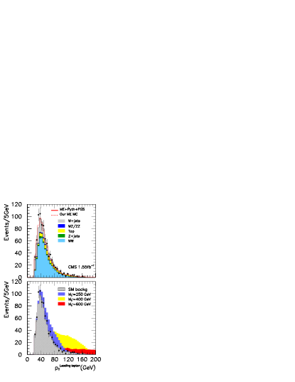
Figure 2: Upper panel: Leading lepton transverse momentum distribution of the SM contributions to the process $pp\to\ell^{+}\ell^{\prime-}/\!\!\!\!E_{T}$ calculated by CMS (colored histograms) together with the number of observed events by CMS (points with error bars) and the performance of ME+Pythia+PGS-MC (red solid) and OUR ME-MC (red dotted). The results shown correspond to an integrated luminosity of $\mathcal{L}=1.55\ \mbox{fb}^{-1}$.
Lower panel: Transverse momentum of the leading lepton for the total SM contribution to the process $pp\to\ell^{+}\ell^{\prime-}/\!\!\!\!E_{T}$ (gray hashed) together with the total expected number of events including a $Z^{\prime}$ of 250 GeV with $G=0.5$ (blue), a $Z^{\prime}$ of 400 GeV with $G=1$ (yellow) and a $Z^{\prime}$ of 600 GeV with $G=1$ (red). For the three masses $\Gamma_{Z^{\prime}}=0.06M_{Z^{\prime}}$. We include also the observed distribution of events in CMS.

The exclusion limits on the production of a $Z^{\prime}$ were extracted using a binned log-likelihood function based on the contents of the bins of the transverse momentum distribution of the leading lepton

$$-2\ln L_{\rm CMS}(M_{Z^{\prime}},G,\Gamma_{Z^{\prime}})=$$

$$\begin{array}[]{c}\\[-5.69046pt] {\rm Min}\\[-5.69046pt] \xi_{j}\end{array}\Big{\{}2\sum_{i=1}^{N^{max}_{CMS}}\left[N^{i}_{B}+N^{i}_{S}-N^{i}_{d}+N^{i}_{d}\log{\frac{N^{i}_{d}}{N^{i}_{B}+N^{i}_{S}}}\right]+$$ (29)

$$+\left(\frac{\xi_{b}^{sy}}{\sigma^{sy}_{b}}\right)^{2}+\left(\frac{\xi_{s}^{sy}}{\sigma^{sy}_{s}}\right)^{2}\Big{\}}\equiv\chi^{2}_{\rm CMS}(M_{Z^{\prime}},G,\Gamma_{Z^{\prime}})$$ (30)

where

$$N^{i}_{B} = N^{i}_{b}\left(1+\xi_{b}^{sy}\right)+N^{i}_{ww}\left(1+\xi_{s}^{sy}\right)$$ (31)

$$N^{i}_{S} = \left(G^{2}N^{i}_{Z^{\prime}}+GN^{i}_{int}\right)\left(1+\xi_{s}^{sy}\right)\;.$$ (32)

Again $N^{i}_{b}$ stands for the number of events expected on the $i$-th bin for the SM processes except for the $W^{+}W^{-}$ contribution, $N^{i}_{ww}$ is the number of events expected on the $i$-th bin for the $W^{+}W^{-}$ contribution, $G^{2}N^{i}_{Z^{\prime}}$ and $GN^{i}_{int}$ are the number of events expected on the $i$-th bin for the pure signal contribution and the interference respectively and $N^{i}_{d}$ is the observed events on the bin $i$.

In the CMS case we make a simplified treatment of the systematic uncertainties in terms of two pulls: $\xi_{b}^{sy}$ is the pull to account for the uncertainty on the expectations for all the SM processes except for the $W^{+}W^{-}$ contribution while $\xi_{s}^{sy}$ is the one to account for the systematic uncertainty on $W^{+}W^{-}$ and the $Z^{\prime}$ new contributions. The standard deviations for these pulls are obtained from CMSwwold :

$$\sigma^{sy}_{b} = 0.20\;,$$ (33)

$$\sigma^{sy}_{s} = 0.08\;.$$ (34)

As for ATLAS we performed two analyses. In the first one we calculate $\ln L_{\rm CMS}$ with the event rates in the 36 leading transverse momentum bins between 20 GeV and 200 GeV (i.e. $N^{max}_{CMS}=36$). In the second analysis we included an extra bin where we sum expected contributions from the $Z^{\prime}$ with $p_{T}^{\rm leading}>200$ GeV (i.e. $N^{max}_{CMS}=37$) and where we assumed that the number of observed events and SM expected predictions for the 37th bin are equal to 0.

Combined Analysis

We also combined the ATLAS and CMS results to get more stringent exclusion limits on the production of a $Z^{\prime}$ by constructing the combined log-likelihood function

$$\chi^{2}_{\rm comb}(M_{Z^{\prime}},G,\Gamma_{Z^{\prime}}) = \chi^{2}_{\rm ATLAS}(M_{Z^{\prime}},G,\Gamma_{Z^{\prime}})$$ (35)

$$+\chi^{2}_{\rm CMS}(M_{Z^{\prime}},G,\Gamma_{Z^{\prime}})$$

where we conservatively assumed that the ATLAS and CMS systematic uncertainties are uncorrelated.

In all cases we set the exclusion 95% (2$\sigma$, 1 d.o.f) limits on $G$ by maximizing the corresponding likelihood function (or equivalently minimizing the $\chi^{2}$) with respect to $G$ for each value of $M_{Z^{\prime}}$ and $\Gamma_{Z^{\prime}}$ and imposing

$$|\chi^{2}(M_{Z^{\prime}},G,\Gamma_{Z^{\prime}})-\chi^{2}_{\rm min}(M_{Z^{\prime}},\Gamma_{Z^{\prime}})|>4\;.$$ (36)

IV Model Independent Results

The $2\sigma$ exclusion limits on possible new states $Z^{\prime}$ derived from $M_{T}$ spectrum observed at the $\mathcal{L}=1.02\ \mbox{fb}^{-1}$ ATLAS data set are depicted in Fig. 3. The results are shown in the plane $G\otimes M_{Z^{\prime}}$ for three possible values of the $Z^{\prime}$ width $\Gamma_{Z^{\prime}}/M_{Z^{\prime}}=0.01$, $0.06$ and $0.3$ as labeled in this figure.

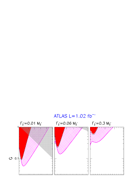
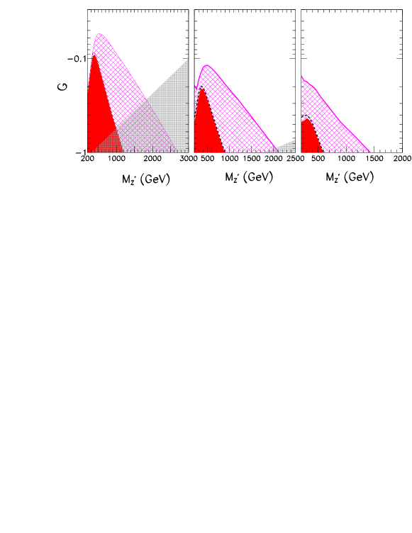
Figure 3: 95% CL exclusion limits on the production of a $Z^{\prime}$ from our analysis of the $M_{T}$ distribution measured by ATLAS with $\mathcal{L}=1.02\ \mbox{fb}^{-1}$ and for three values of $\Gamma_{Z^{\prime}}/M_{Z^{\prime}}=0.01$, $0.06$ and $0.3$ (left, center and right panels respectively). The red solid regions are derived using the log-likelihood function in Eq. (17) with $N^{max}_{AT}=15$. The regions bounded by the black dashed curves correspond to the same analysis removing the effect of the systematic pulls. The purple hatched regions are derived using the log-likelihood function in Eq. (17) with $N^{max}_{AT}=16$. The shadowed regions in the upper (lower) right corner of the upper (lower) panels represent the excluded values by the condition Eq. (3).

The red solid regions in Fig. 3 were derived using the log-likelihood function in Eq. (17) with $N^{max}_{AT}=15$, i.e. with the 15 bins of the transverse mass distribution between $M_{T}=40$ GeV and $M_{T}=340$ GeV. Comparing the left, central and right panels one observes that, as expected, bounds are stronger for narrow resonances. The shadowed regions in the upper (lower) right corner of the upper (lower) panels of this figure represents the excluded values by the condition Eq. (3).

In order to illustrate the effect of the systematic uncertainties included in this analysis we also show the black dashed curves which correspond to the same analysis but fixing the pulls to zero. As seen by comparing the dashed curve with the boundary of the solid region, the bounds are dominated by statistics for the available integrated luminosity and the inclusion of the systematic uncertainties have a very limited impact.

The sensitivity reach when a non-zero observation for $M_{T}>340$ GeV is included as a 16th bin, is shown as the purple hatched regions. The effect of the inclusion of this additional bin is more important the heavier and the wider $Z^{\prime}$ is. This is due to the fact that a heavier and/or wider $Z^{\prime}$ gives a larger contribution to events with $M_{T}>340$ GeV. Finally the difference between the regions in the upper and lower panels arises from the interference between the SM and $Z^{\prime}$ contribution. As expected this effect is only relevant for the lighter and wider $Z^{\prime}$ since the interference term is roughly proportional to $\Gamma_{Z^{\prime}}/M_{Z^{\prime}}$.

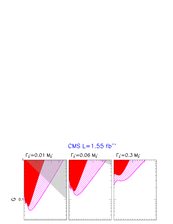
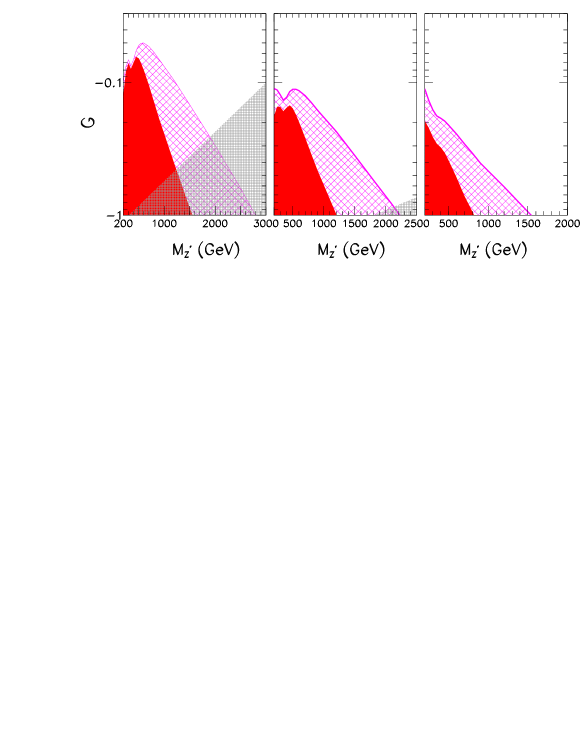
Figure 4: 95% CL exclusion limits on the production of a $Z^{\prime}$ from our analysis of the $p_{T}^{\rm leading}$ distribution measured by CMS with $\mathcal{L}=1.55\ \mbox{fb}^{-1}$. The left, center and right panels correspond to three values of $\Gamma_{Z^{\prime}}/M_{Z^{\prime}}=0.01$ ,$0.06$ and $0.3$ respectively. The red solid regions are derived using the log-likelihood function in Eq. (30) with $N^{max}_{CMS}=36$. The purple hatched regions are derived using the log-likelihood function in Eq. (30) with $N^{max}_{CMS}=37$. The shadowed regions in the upper (lower) right corner of the upper (lower) panels represent the excluded values by the condition Eq. (3).

The $2\sigma$ exclusion limits on the production of a $Z^{\prime}$ derived from our analysis of the $p_{T}^{\rm leading}$ distribution measured by CMS with $\mathcal{L}=1.55\ \mbox{fb}^{-1}$ can be seen in Fig. 4. The dependence of the excluded range of $G$ on the $Z^{\prime}$ mass and width is similar to Fig. 3 as expected. The only difference is associated with the larger event sample. As no positive signal is observed neither in ATLAS nor in CMS, the bounds obtained from our analysis of the CMS data are stronger than for the ATLAS due to the larger integrated luminosity used in the former.

Finally in Fig. 5 we present the exclusion constraints on the production of a new neutral vector resonance from our combined analysis of the measured $M_{T}$ distribution in ATLAS with $\mathcal{L}=1.02\ \mbox{fb}^{-1}$ and the $p_{T}^{\rm leading}$ distribution measured by CMS with $\mathcal{L}=1.55\ \mbox{fb}^{-1}$. We see that the combination of ATLAS and CMS data have already excluded a sizable region of the parameter space for the production of new spin-1 $Z^{\prime}$ associated with the EWSB sector. In particular, from our analysis with 15 and 36 (16 and 37) bins of the ATLAS and CMS distributions, a narrow resonance of any mass with $\Gamma_{Z^{\prime}}/M_{Z^{\prime}}=0.01$ and that saturates the partial wave amplitude for the process $W^{+}W^{-}\to W^{+}W^{-}$, is excluded at 95% CL if its coupling to the light quarks is larger than 45% (22%) of the SM $Z\bar{q}q$ coupling. Moreover, our analysis with 15 and 36 bins of the ATLAS and CMS distributions, excludes at 95% CL a wider resonance with $\Gamma_{Z^{\prime}}/M_{Z^{\prime}}=0.06$ $(0.3)$ that saturates the partial wave amplitude for the process $W^{+}W^{-}\to W^{+}W^{-}$ and couples to light quarks with SM strength if $M_{Z^{\prime}}\leq 1250\,(850)$ GeV. From the extended analysis using 16 and 37 bins of the ATLAS and CMS distributions we find that no such SM coupling resonance is allowed for any mass for $\Gamma_{Z^{\prime}}/M_{Z^{\prime}}=0.06$ or $M_{Z^{\prime}}<1750$ GeV for $\Gamma_{Z^{\prime}}/M_{Z^{\prime}}=0.3$.

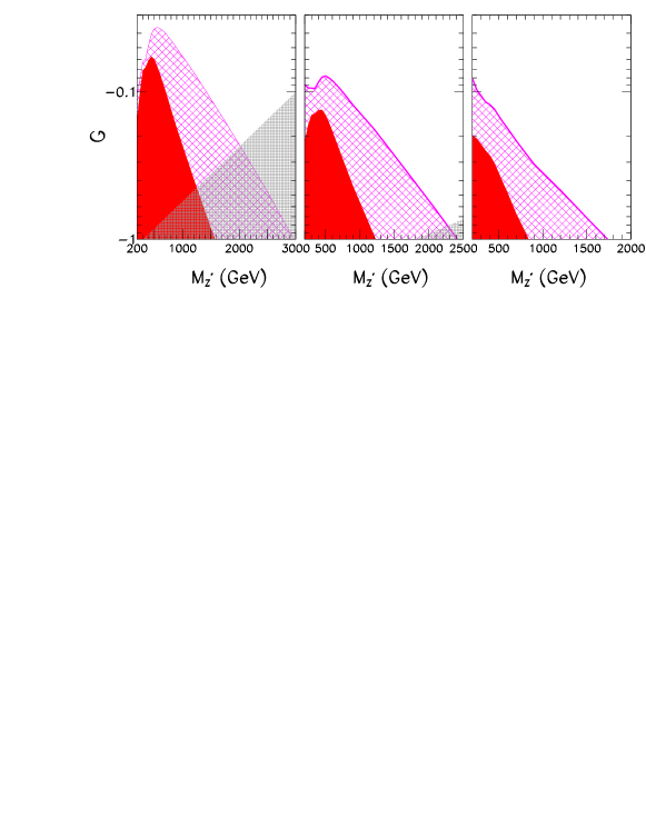
Figure 5: 95% CL exclusion limits on the production of a $Z^{\prime}$ from our combined analysis of the measured $M_{T}$ distribution in ATLAS with $\mathcal{L}=1.02\ \mbox{fb}^{-1}$ and the $p_{T}^{\rm leading}$ distribution measured by CMS with $\mathcal{L}=1.55\ \mbox{fb}^{-1}$. The red solid (purple hatched) regions are derived using the log-likelihood defined in Eq. (35) with 15 and 36 (16 and 37) bins of the ATLAS and CMS distributions respectively. The shadowed regions in the upper (lower) right corner of the upper (lower) panels represent the excluded values by the condition Eq. (3).

At this point it is interesting to compare our $Z^{\prime}$ bounds with the ones obtained by the CDF collaboration analyzing $WW$ production at the Tevatron cdf in the framework of the Sequential Standard Model SSM . In the CDF analysis our coupling $G$ is related to the parameter $\xi$ as $G=\xi\sqrt{3}M_{Z^{\prime}}/M_{Z}$ while the $Z^{\prime}$ width is a well defined function of $\xi$ and $M_{Z^{\prime}}$. Generically this lead to a narrow $Z^{\prime}$s with $\Gamma_{Z^{\prime}}/M_{Z^{\prime}}\lesssim 0.1$. For $Z^{\prime}$ masses of 250, 600 and 950 GeV the CDF constraints read $|G|<0.47$, $0.27$ and $1.36$ respectively. On the other hand our analyses without (with) extra bins lead to bounds $|G|<0.20$, $0.12$ and $0.60$ ($0.18$, $0.067$,$0.15$) for the same masses. In conclusion, translating our bounds into the model used by CDF we get that generically the constraints from our most conservative analysis of the ATLAS and CMS distributions, i.e. without the extra bins, extend the CDF exclusion to couplings about a factor 2 smaller for the accessible mass range at Tevatron $M_{Z^{\prime}}\lesssim 950$. Furthermore, our results also widen the accessible $M_{Z^{\prime}}$ mass range.

V Model dependent results

The above analyses can be used to place bounds on specific models once we take into account its couplings. Generically within a given model the width of the vector resonance and the strength of its couplings to fermions and gauge bosons can be functions of a few parameters. As an illustration we made a dedicated study of the bounds attainable in the framework recently proposed in Ref. grojean that exhibits a single vector $SU(2)_{\rm custodial}$–triplet resonance that is included to saturate the unitarization condition. In brief in this case the couplings of the resonance to the fermions as well as to the gauge bosons can be cast in terms of a unique parameter $g_{\rho\pi\pi}$ with the decay into gauge bosons being the dominant mode. The other free parameter is the mass of the new resonance $M_{\rho}=M_{Z^{\prime}}$. The limits derived in the previous section can not be directly applied to this case since the $Z^{\prime}$ couplings to quarks differs from the SM ones. In this example we generated the ${\cal O}(\alpha^{4})$ amplitudes using MADGRAPH. The constraints in this scenario coming from the reaction  1 are shown in Fig. 6 and they represent the strongest bounds at present on this scenario.

Because of the existence of an associated charged resonance associated to the unitarization of the channel $WZ\to WZ$, bounds can be also imposed from the searches of $pp\rightarrow ZW^{\pm}$ such as the one performed by the CMS collaboration CMSW' . CMS present the results of their negative searches for $W^{\prime}$ in the framework of the Sequential Standard Model SSM as constraints on $\sigma(pp\rightarrow W^{\prime})\times Br(W^{\prime}\rightarrow 3l\nu)$. In Ref. grojean a simplified adaptation of this CMS bound was made which seemed to exclude $M_{\rho}<900$ GeV for all values of $g_{\rho\pi\pi}>1$. However one must notice that despite the bounds in Ref. CMSW' are presented in a seemingly “model independent” form, the actual efficiency for reconstruction of their resonance signal depends on the assumed width of the resonance which depends on the model assumed.

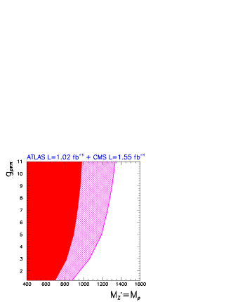
Figure 6: 95% CL exclusion limits from our combined analysis of the measured $M_{T}$ distribution in ATLAS with $\mathcal{L}=1.02\ \mbox{fb}^{-1}$ and the $p_{T}^{\rm leading}$ distribution measured by CMS with $\mathcal{L}=1.55\ \mbox{fb}^{-1}$ in the framework of the model in Ref. grojean . The red solid (purple hatched) regions are derived using the log-likelihood defined in Eq. (35) with 15 and 36 (16 and 37) bins of the ATLAS and CMS distributions respectively.

VI Summary

In this work we have presented an analysis of the ATLAS ATLASww and CMS CMSww kinematic distributions of the $pp\to\ell^{+}\ell^{\prime-}/\!\!\!\!E_{T}$ events to place bounds on the production of a $Z^{\prime}$ associated with the EWSB sector which contributes to the above final state via $pp\to Z^{\prime}\to W^{+}W^{-}\to\ell^{+}\ell^{\prime-}\,/\!\!\!\!E_{T}$.

To make our study as model independent as possible we kept as independent parameters the coupling strength of the $Z^{\prime}$ to light quarks, to the gauge bosons, its width, and its mass. We have set exclusion bounds by looking at the different behaviour of the SM processes and $Z^{\prime}$ new contributions with respect to two kinematical variables; the transverse momentum of the leading lepton for the CMS case and the transverse mass of the system for the ATLAS one as a function of the three free parameters in the study. The results are shown in Figs. 3 and Figs. 4 for the study of the measured distribution of events in ATLAS with integrated luminosity of $\mathcal{L}=1.02\mbox{fb}^{-1}$ and in CMS with integrated luminosity of $\mathcal{L}=1.55\ \mbox{fb}^{-1}$ respectively. We have also combined the likelihoods for the two analyses to get the more stringent combined exclusion limits shown in Fig. 5.

We observe that the combined analysis already excludes a large region of the parameter space for the lightest masses, well exceeding the limits from Tevatron. Moreover, we also showed how our analysis framework can be adapted to specific models.

References

- (1) B. W. Lee, C. Quigg and H. B. Thacker, Phys. Rev. D 16, 1519 (1977).
- (2) S. Dimopoulos and L. Susskind, Nucl. Phys. B 155, 237 (1979); L. Susskind, Phys. Rev. D 20, 2619 (1979); S. Weinberg, Phys. Rev. D 19, 1277 (1979).
- (3) See for instance, C. T. Hill and E. H. Simmons, Phys. Rept. 381, 235 (2003) [Erratum-ibid. 390, 553 (2004)] [arXiv:hep-ph/0203079];
- (4) C. Csaki, C. Grojean, H. Murayama, L. Pilo and J. Terning, Phys. Rev. D 69, 055006 (2004) [arXiv:hep-ph/0305237]; C. Csaki, C. Grojean, L. Pilo and J. Terning, Phys. Rev. Lett. 92, 101802 (2004) [arXiv:hep-ph/0308038]; Y. Nomura, JHEP 0311, 050 (2003) [arXiv:hep-ph/0309189]; C. Csaki, C. Grojean, J. Hubisz, Y. Shirman and J. Terning, Phys. Rev. D 70, 015012 (2004) [arXiv:hep-ph/0310355]; G. Cacciapaglia, C. Csaki, G. Marandella and J. Terning, Phys. Rev. D 75, 015003 (2007) [arXiv:hep-ph/0607146]; C. Csaki and D. Curtin, arXiv:0904.2137 [hep-ph].
- (5) C. Csaki, C. Grojean, H. Murayama, L. Pilo and J. Terning, Phys. Rev. D 69, 055006 (2004) [arXiv:hep-ph/0305237].
- (6) N. Arkani-Hamed, M. Porrati and L. Randall, JHEP 0108, 017 (2001) [arXiv:hep-th/0012148]; R. Rattazzi and A. Zaffaroni, JHEP 0104, 021 (2001) [arXiv:hep-th/0012248]; M. Perez-Victoria, JHEP 0105, 064 (2001) [arXiv:hep-th/0105048].
- (7) A. Alves, O. J. P. Eboli, D. Goncalves et al., Phys. Rev. D80, 073011 (2009). [arXiv:0907.2915 [hep-ph]].
- (8) O. J. P. Eboli, C. S. Fong, J. Gonzalez-Fraile, M. C. Gonzalez-Garcia, Phys. Rev. D83, 095014 (2011). [arXiv:1102.3429 [hep-ph]].
- (9) A. Birkedal, K. Matchev and M. Perelstein, Phys. Rev. Lett. 94, 191803 (2005) [arXiv:hep-ph/0412278]; H. J. He et al., Phys. Rev. D 78, 031701 (2008) [arXiv:0708.2588 [hep-ph]]; T. Ohl and C. Speckner, Phys. Rev. D 78, 095008 (2008) [arXiv:0809.0023 [hep-ph]].
- (10) The ATLAS Collaboration, ATLAS-CONF-2011-110
-
(11)
The CMS Collaboration
CMS-HIG-11-014
https://twiki.cern.ch/twiki/bin/view
/CMSPublic/Hig11014TWiki
- (12) T. Stelzer and F. Long, Comput. Phys. Commun. 81 (1994) 357; F. Maltoni and T. Stelzer, J. High Energy Phys. 0302, 027 (2003) [arXiv:hep-ph/0208156].
- (13) T. Sjostrand, S. Mrenna, P. Z. Skands, JHEP 0605, 026 (2006). [hep-ph/0603175].
-
(14)
John Conway, PGS 4,
https://physics.ucdavis.edu/~conway/research
/software/pgs/pgs4-support.htm
- (15) J. Pumplin, D. R. Stump, J. Huston, H. L. Lai, P. Nadolsky and W. K. Tung, JHEP 0207, 012 (2002) [arXiv:hep-ph/0201195].
- (16) M. Cacciari, G. P. Salam and G. Soyez, JHEP 0804 (2008) 063 [arXiv:0802.1189 [hep-ph]].
- (17) G. L. Fogli, E. Lisi, A. Marrone, D. Montanino, A. Palazzo, Phys. Rev. D66, 053010 (2002). [hep-ph/0206162], M. C. Gonzalez-Garcia, M. Maltoni, Phys. Rept. 460, 1-129 (2008). [arXiv:0704.1800 [hep-ph]].
- (18) The CMS Collaboration CMS-EWK-11-010
- (19) T. Aaltonen et al. [ The CDF Collaboration ], Phys. Rev. Lett. 104, 241801 (2010). [arXiv:1004.4946 [hep-ex]].
- (20) J.C. Pati and A. Salam, Phys. Rev. D 10, 275 (1974); Phys. Rev. D 11, 703 (1974).
- (21) A. Falkowski, C. Grojean, A. Kaminska, S. Pokorski and A. Weiler, JHEP 1111, 028 (2011) [arXiv:1108.1183 [hep-ph]].
- (22) The CMS Collaboration CMS-PAS-EXO-11-041