March 2006 Arch. Comput. Meth. Engng. Vol. 00, 0, 1-76 (2006)  Archives of Computational
Methods in Engineering
State of the art reviews  

Automating the Finite Element Method

Anders Logg

Toyota Technological Institute at Chicago

University Press Building

1427 East 60th Street

Chicago, Illinois 60637 USA

Email: logg@tti-c.org

Summary

The finite element method can be viewed as a machine that automates the discretization of differential equations, taking as input a variational problem, a finite element and a mesh, and producing as output a system of discrete equations. However, the generality of the framework provided by the finite element method is seldom reflected in implementations (realizations), which are often specialized and can handle only a small set of variational problems and finite elements (but are typically parametrized over the choice of mesh).

This paper reviews ongoing research in the direction of a complete automation of the finite element method. In particular, this work discusses algorithms for the efficient and automatic computation of a system of discrete equations from a given variational problem, finite element and mesh. It is demonstrated that by automatically generating and compiling efficient low-level code, it is possible to parametrize a finite element code over variational problem and finite element in addition to the mesh.

1 INTRODUCTION

The finite element method (Galerkin’s method) has emerged as a universal method for the solution of differential equations. Much of the success of the finite element method can be contributed to its generality and simplicity, allowing a wide range of differential equations from all areas of science to be analyzed and solved within a common framework. Another contributing factor to the success of the finite element method is the flexibility of formulation, allowing the properties of the discretization to be controlled by the choice of finite element (approximating spaces).

At the same time, the generality and flexibility of the finite element method has for a long time prevented its automation, since any computer code attempting to automate it must necessarily be parametrized over the choice of variational problem and finite element, which is difficult. Consequently, much of the work must still be done by hand, which is both tedious and error-prone, and results in long development times for simulation codes.

Automating systems for the solution of differential equations are often met with skepticism, since it is believed that the generality and flexibility of such tools cannot be combined with the efficiency of competing specialized codes that only need to handle one equation for a single choice of finite element. However, as will be demonstrated in this paper, by automatically generating and compiling low-level code for any given equation and finite element, it is possible to develop systems that realize the generality and flexibility of the finite element method, while competing with or outperforming specialized and hand-optimized codes.

1.1 Automating the Finite Element Method

To automate the finite element method, we need to build a machine that takes as input a discrete variational problem posed on a pair of discrete function spaces defined by a set of finite elements on a mesh, and generates as output a system of discrete equations for the degrees of freedom of the solution of the variational problem. In particular, given a discrete variational problem of the form: Find $U\in V_{h}$ such that

$$a(U;v)=L(v)\quad\forall v\in\hat{V}_{h},$$ (1)

where $a:V_{h}\times\hat{V}_{h}\rightarrow\mathbb{R}$ is a semilinear form which is linear in its second argument, $L:\hat{V}_{h}\rightarrow\mathbb{R}$ a linear form and $(\hat{V}_{h},V_{h})$ a given pair of discrete function spaces (the test and trial spaces), the machine should automatically generate the discrete system

$$F(U)=0,$$ (2)

where $F:V_{h}\rightarrow\mathbb{R}^{N}$, $N=|\hat{V}_{h}|=|V_{h}|$ and

$$F_{i}(U)=a(U;\hat{\phi}_{i})-L(\hat{\phi}_{i}),\quad i=1,2,\ldots,N,$$ (3)

for $\{\hat{\phi}_{i}\}_{i=1}^{N}$ a given basis for $\hat{V}_{h}$.

Typically, the discrete variational problem (1) is obtained as the discrete version of a corresponding continuous variational problem: Find $u\in V$ such that

$$a(u;v)=L(v)\quad\forall v\in\hat{V},$$ (4)

where $\hat{V}_{h}\subset\hat{V}$ and $V_{h}\subset V$.

The machine should also automatically generate the discrete representation of the linearization of the given semilinear form $a$, that is the matrix $A\in\mathbb{R}^{N\times N}$ defined by

$$A_{ij}(U)=a^{\prime}(U;\hat{\phi}_{i},\phi_{j}),\quad i,j=1,2,\ldots,N,$$ (5)

where $a^{\prime}:V_{h}\times\hat{V}_{h}\times V_{h}\rightarrow\mathbb{R}$ is the Fréchet derivative of $a$ with respect to its first argument and $\{\hat{\phi}_{i}\}_{i=1}^{N}$ and $\{\phi_{i}\}_{i=1}^{N}$ are bases for $\hat{V}_{h}$ and $V_{h}$ respectively.

In the simplest case of a linear variational problem,

$$a(v,U)=L(v)\quad\forall v\in\hat{V}_{h},$$ (6)

the machine should automatically generate the linear system

$$AU=b,$$ (7)

where $A_{ij}=a(\hat{\phi}_{i},\phi_{j})$ and $b_{i}=L(\hat{\phi}_{i})$, and where $(U_{i})\in\mathbb{R}^{N}$ is the vector of degrees of freedom for the discrete solution $U$, that is, the expansion coefficients in the given basis for $V_{h}$,

$$U=\sum_{i=1}^{N}U_{i}\phi_{i}.$$ (8)

We return to this in detail below and identify the key steps towards a complete automation of the finite element method, including algorithms and prototype implementations for each of the key steps.

1.2 The FEniCS Project and the Automation of CMM

The FEniCS project [60, 36] was initiated in 2003 with the explicit goal of developing free software for the Automation of Computational Mathematical Modeling (CMM), including a complete automation of the finite element method. As such, FEniCS serves as a prototype implementation of the methods and principles put forward in this paper.

In [96], an agenda for the automation of CMM is outlined, including the automation of (i) discretization, (ii) discrete solution, (iii) error control, (iv) modeling and (v) optimization. The automation of discretization amounts to the automatic generation of the system of discrete equations (2) or (7) from a given given differential equation or variational problem. Choosing as the foundation for the automation of discretization the finite element method, the first step towards the Automation of CMM is thus the automation of the finite element method. We continue the discussion on the automation of CMM below in Section 11.

Since the initiation of the FEniCS project in 2003, much progress has been made, especially concerning the automation of discretization. In particular, two central components that automate central aspects of the finite element method have been developed. The first of these components is FIAT, the FInite element Automatic Tabulator [83, 82, 84], which automates the generation of finite element basis functions for a large class of finite elements. The second component is FFC, the FEniCS Form Compiler [98, 87, 88, 99], which automates the evaluation of variational problems by automatically generating low-level code for the assembly of the system of discrete equations from given input in the form of a variational problem and a (set of) finite element(s).

In addition to FIAT and FFC, the FEniCS project develops components that wrap the functionality of collections of other FEniCS components (middleware) to provide simple, consistent and intuitive user interfaces for application programmers. One such example is DOLFIN [62, 68, 63], which provides both a C++ and a Python interface (through SWIG [15, 14]) to the basic functionality of FEniCS.

We give more details below in Section 9 on FIAT, FFC, DOLFIN and other FEniCS components, but list here some of the key properties of the software components developed as part of the FEniCS project, as well as the FEniCS system as a whole:

• automatic and efficient evaluation of variational problems through FFC [98, 87, 88, 99], including support for arbitrary mixed formulations;

• automatic and efficient assembly of systems of discrete equations through DOLFIN [62, 68, 63];

• support for general families of finite elements, including continuous and discontinuous Lagrange finite elements of arbitrary degree on simplices through FIAT [83, 82, 84];

• high-performance parallel linear algebra through PETSc [9, 8, 10];

• arbitrary order multi-adaptive $\mathrm{mcG}(q)$/$\mathrm{mdG}(q)$ and mono-adaptive $\mathrm{cG}(q)$/$\mathrm{dG}(q)$ ODE solvers [94, 95, 50, 97, 100].

1.3 Automation and Mathematics Education

By automating mathematical concepts, that is, implementing corresponding concepts in software, it is possible to raise the level of the mathematics education. An aspect of this is the possibility of allowing students to experiment with mathematical concepts and thereby obtaining an increased understanding (or familiarity) for the concepts. An illustrative example is the concept of a vector in $\mathbb{R}^{n}$, which many students get to know very well through experimentation and exercises in Octave [37] or MATLAB [118]. If asked which is the true vector, the $x$ on the blackboard or the x on the computer screen, many students (and the author) would point towards the computer.

By automating the finite element method, much like linear algebra has been automated before, new advances can be brought to the mathematics education. One example of this is Puffin [70, 69], which is a minimal and educational implementation of the basic functionality of FEniCS for Octave/MATLAB. Puffin has successfully been used in a number of courses at Chalmers in Göteborg and the Royal Institute of Technology in Stockholm, ranging from introductory undergraduate courses to advanced undergraduate/beginning graduate courses. Using Puffin, first-year undergraduate students are able to design and implement solvers for coupled systems of convection–diffusion–reaction equations, and thus obtaining important understanding of mathematical modeling, differential equations, the finite element method and programming, without reducing the students to button-pushers.

Using the computer as an integrated part of the mathematics education constitutes a change of paradigm [67], which will have profound influence on future mathematics education.

1.4 Outline

This paper is organized as follows. In the next section, we first present a survey of existing finite element software that automate particular aspects of the finite element method. In Section 3, we then give an introduction to the finite element method with special emphasis on the process of generating the system of discrete equations from a given variational problem, finite element(s) and mesh. A summary of the notation can be found at the end of this paper.

Having thus set the stage for our main topic, we next identify in Sections 4–6 the key steps towards an automation of the finite element method and present algorithms and systems that accomplish (in part) the automation of each of these key steps. We also discuss a framework for generating an optimized computation from these algorithms in Section 7. In Section 8, we then highlight a number of important concepts and techniques from software engineering that play an important role for the automation of the finite element method.

Prototype implementations of the algorithms are then discussed in Section 9, including benchmark results that demonstrate the efficiency of the algorithms and their implementations. We then, in Section 10, present a number of examples to illustrate the benefits of a system automating the finite element method. As an outlook towards further research, we present in Section 11 an agenda for the development of an extended automating system for the Automation of CMM, for which the automation of the finite element method plays a central role. Finally, we summarize our findings in Section 12.

2 SURVEY OF CURRENT FINITE ELEMENT SOFTWARE

There exist today a number of projects that seek to create systems that (in part) automate the finite element method. In this section, we survey some of these projects. A complete survey is difficult to make because of the large number of such projects. The survey is instead limited to a small set of projects that have attracted the attention of the author. In effect, this means that most proprietary systems have been excluded from this survey.

It is instructional to group the systems both by their level of automation and their design. In particular, a number of systems provide automated generation of the system of discrete equations from a given variational problem, which we in this paper refer to as the automation of the finite element method or automatic assembly, while other systems only provide the user with a basic toolkit for this purpose. Grouping the systems by their design, we shall differentiate between systems that provide their functionality in the form of a library in an existing language and systems that implement new domain-specific languages for finite element computation. A summary for the surveyed systems is given in Table 1.

It is also instructional to compare the basic specification of a simple test problem such as Poisson’s equation, $-\Delta u=f$ in some domain $\Omega\subset\mathbb{R}^{d}$, for the surveyed systems, or more precisely, the specification of the corresponding discrete variational problem $a(v,U)=L(v)$ for all $v$ in some suitable test space, with the bilinear form $a$ given by

$$a(v,U)=\int_{\Omega}\nabla v\cdot\nabla U\,\mathrm{d}x,$$ (9)

and the linear form $L$ given by

$$L(v)=\int_{\Omega}v\,f\,\mathrm{d}x.$$ (10)

Each of the surveyed systems allow the specification of the variational problem for Poisson’s equation with varying degree of automation. Some of the systems provide a high level of automation and allow the variational problem to be specified in a notation that is very close to the mathematical notation used in (9) and (10), while others require more user-intervention. In connection to the presentation of each of the surveyed systems below, we include as an illustration the specification of the variational problem for Poisson’s equation in the notation employed by the system in question. In all cases, we include only the part of the code essential to the specification of the variational problem. Since the different systems are implemented in different languages, sometimes even providing new domain-specific languages, and since there are differences in philosophies, basic concepts and capabilities, it is difficult to make a uniform presentation. As a result, not all the examples specify exactly the same problem.

Project	automatic assembly	library / language	license
Analysa	yes	language	proprietary
deal.II	no	library	QPL
Diffpack	no	library	proprietary
FEniCS	yes	both	GPL, LGPL
FreeFEM	yes	language	LGPL
GetDP	yes	language	GPL
Sundance	yes	library	LGPL

Table 1: Summary of projects seeking to automate the finite element method.

2.1 Analysa

Analysa [6, 7] is a domain-specific language and problem-solving environment (PSE) for partial differential equations. Analysa is based on the functional language Scheme and provides a language for the definition of variational problems. Analysa thus falls into the category of domain-specific languages.

Analysa puts forward the idea that it is sometimes desirable to compute the action of a bilinear form, rather than assembling the matrix representing the bilinear form in the current basis. In the notation of [7], the action of a bilinear form $a:\hat{V}_{h}\times V_{h}\rightarrow\mathbb{R}$ on a given discrete function $U\in V_{h}$ is

$$w=a(\hat{V}_{h},U)\in\mathbb{R}^{N},$$ (11)

where

$$w_{i}=a(\hat{\phi}_{i},U),\quad i=1,2,\ldots,N.$$ (12)

Of course, we have $w=AU$, where $A$ is the matrix representing the bilinear form, with $A_{ij}=a(\hat{\phi}_{i},\phi_{j})$, and $(U_{i})\in\mathbb{R}^{N}$ is the vector of expansion coefficients for $U$ in the basis of $V_{h}$. It follows that

$$w=a(\hat{V}_{h},U)=a(\hat{V}_{h},V_{h})U.$$ (13)

If the action only needs to be evaluated a few times for different discrete functions $U$ before updating a linearization (reassembling the matrix $A$), it might be more efficient to compute each action directly than first assembling the matrix $A$ and applying it to each $U$.

To specify the variational problem for Poisson’s equation with Analysa, one specifies a pair of bilinear forms a and m, where a represents the bilinear form $a$ in (9) and m represents the bilinear form

$$m(v,U)=\int_{\Omega}v\,U\,\mathrm{d}x,$$ (14)

corresponding to a mass matrix. In the language of Analysa, the linear form $L$ in (10) is represented as the application of the bilinear form $m$ on the test space $\hat{V}_{h}$ and the right-hand side $f$,

$$L(\hat{\phi}_{i})=m(\hat{V}_{h},f)_{i},\quad i=1,2,\ldots,N,$$ (15)

as shown in Table 2. Note that Analysa thus defers the coupling of the forms and the test and trial spaces until the computation of the system of discrete equations.

      (integral-forms     ((a v U) (dot (gradient v) (gradient U)))     ((m v U) (* v U))   )     (elements     (element (lagrange-simplex 1))   )     (spaces     (test-space (fe element (all mesh) r:))     (trial-space (fe element (all mesh) r:))   )     (functions     (f (interpolant test-space (...)))   )     (define A-matrix (a testspace trial-space))   (define b-vector (m testspace f))     

Table 2: Specifying the variational problem for Poisson’s equation with Analysa using piecewise linear elements on simplices (triangles or tetrahedra).

2.2 deal.II

deal.II [12, 13, 11] is a C++ library for finite element computation. While providing tools for finite elements, meshes and linear algebra, deal.II does not provide support for automatic assembly. Instead, a user needs to supply the complete code for the assembly of the system (7), including the explicit computation of the element stiffness matrix (see Section 3 below) by quadrature, and the insertion of each element stiffness matrix into the global matrix, as illustrated in Table 3. This is a common design for many finite element libraries, where the ambition is not to automate the finite element method, but only to provide a set of basic tools.

      ...   for (dof_handler.begin_active(); cell! = dof_handler.end(); ++cell)   {     ...     for (unsigned int i = 0; i < dofs_per_cell; ++i)       for (unsigned int j = 0; j < dofs_per_cell; ++j)         for (unsigned int q_point = 0; q_point < n_q_points; ++q_point)           cell_matrix(i, j) += (fe_values.shape_grad (i, q_point) *                                 fe_values.shape_grad (j, q_point) *                                 fe_values.JxW(q_point));       for (unsigned int i = 0; i < dofs_per_cell; ++i)       for (unsigned int q_point = 0; q_point < n_q_points; ++q_point)         cell_rhs(i) += (fe_values.shape_value (i, q_point) *                         <value of right-hand side f> *                         fe_values.JxW(q_point));       cell->get_dof_indices(local_dof_indices);       for (unsigned int i = 0; i < dofs_per_cell; ++i)       for (unsigned int j = 0; j < dofs_per_cell; ++j)         system_matrix.add(local_dof_indices[i],                           local_dof_indices[j],                           cell_matrix(i, j));       for (unsigned int i = 0; i < dofs_per_cell; ++i)       system_rhs(local_dof_indices[i]) += cell_rhs(i);   }   ...     

Table 3: Assembling the linear system (7) for Poisson’s equation with deal.II.

2.3 Diffpack

Diffpack [24, 92] is a C++ library for finite element and finite difference solution of partial differential equations. Initiated in 1991, in a time when most finite element codes were written in FORTRAN, Diffpack was one of the pioneering libraries for scientific computing with C++. Although originally released as free software, Diffpack is now a proprietary product.

Much like deal.II, Diffpack requires the user to supply the code for the computation of the element stiffness matrix, but automatically handles the loop over quadrature points and the insertion of the element stiffness matrix into the global matrix, as illustrated in Table 4.

      for (int i = 1; i <= nbf; i++)     for (int j = 1; j <= nbf; j++)       elmat.A(i, j) += (fe.dN(i, 1) * fe.dN(j, 1) +                         fe.dN(i, 2) * fe.dN(j, 2) +                         fe.dN(i, 3) * fe.dN(j, 3)) * detJxW;     for (int i = 1; i <= nbf; i++)     elmat.b(i) += fe.N(i)*<value of right-hand side f>*detJxW;     

Table 4: Computing the element stiffness matrix and element load vector for Poisson’s equation with Diffpack.

2.4 FEniCS

The FEniCS project [60, 36] is structured as a system of interoperable components that automate central aspects of the finite element method. One of these components is the form compiler FFC [98, 87, 88, 99], which takes as input a variational problem together with a set of finite elements and generates low-level code for the automatic computation of the system of discrete equations. In this regard, the FEniCS system implements a domain-specific language for finite element computation, since the form is entered in a special language interpreted by the compiler. On the other hand, the form compiler FFC is also available as a Python module and can be used as a just-in-time (JIT) compiler, allowing variational problems to be specified and computed with from within the Python scripting environment. The FEniCS system thus falls into both categories of being a library and a domain-specific language, depending on which interface is used.

To specify the variational problem for Poisson’s equation with FEniCS, one must specify a pair of basis functions v and U, the right-hand side function f, and of course the bilinear form a and the linear form L, as shown in Table 5.

      element = FiniteElement(‘‘Lagrange’’, ‘‘tetrahedron’’, 1)     v = BasisFunction(element)   U = BasisFunction(element)   f = Function(element)     a = dot(grad(v), grad(U))*dx   L = v*f*dx     

Table 5: Specifying the variational problem for Poisson’s equation with FEniCS using piecewise linear elements on tetrahedra.

Note in Table 5 that the function spaces (finite elements) for the test and trial functions v and U together with all additional functions/coefficients (in this case the right-hand side f) are fixed at compile-time, which allows the generation of very efficient low-level code since the code can be generated for the specific given variational problem and the specific given finite element(s).

Just like Analysa, FEniCS (or FFC) supports the specification of actions, but while Analysa allows the specification of a general expression that can later be treated as a bilinear form, by applying it to a pair of function spaces, or as a linear form, by applying it to a function space and a given fixed function, the arity of the form must be known at the time of specification in the form language of FFC. As an example, the specification of a linear form a representing the action of the bilinear form (9) on a function U is given in Table 6.

      element = FiniteElement(‘‘Lagrange’’, ‘‘tetrahedron’’, 1)     v = BasisFunction(element)   U = Function(element)     a = dot(grad(v), grad(U))*dx     

Table 6: Specifying the linear form for the action of the bilinear form (9) with FEniCS using piecewise linear elements on tetrahedra.

A more detailed account of the various components of the FEniCS project is given below in Section 9.

2.5 FreeFEM

FreeFEM [108, 59] implements a domain-specific language for finite element solution of partial differential equations. The language is based on C++, extended with a special language that allows the specification of variational problems. In this respect, FreeFEM is a compiler, but it also provides an integrated development environment (IDE) in which programs can be entered, compiled (with a special compiler) and executed. Visualization of solutions is also provided.

FreeFEM comes in two flavors, the current version FreeFEM++ which only supports 2D problems and the 3D version FreeFEM3D. Support for 3D problems will be added to FreeFEM++ in the future. [108].

To specify the variational problem for Poisson’s equation with FreeFEM++, one must first define the test and trial spaces (which we here take to be the same space V), and then the test and trial functions v and U, as well as the function f for the right-hand side. One may then define the bilinear form a and linear form L as illustrated in Table 7.

      fespace V(mesh, P1);   V v, U;   func f = ...;     varform a(v, U) = int2d(mesh)(dx(v)*dx(U) + dy(v)*dy(U));   varform L(v) = int2d(mesh)(v*f);     

Table 7: Specifying the variational problem for Poisson’s equation with FreeFEM++ using piecewise linear elements on triangles (as determined by the mesh).

2.6 GetDP

GetDP [35, 34] is a finite element solver which provides a special declarative language for the specification of variational problems. Unlike FreeFEM, GetDP is not a compiler, nor is it a library, but it will be classified here under the category of domain-specific languages. At start-up, GetDP parses a problem specification from a given input file and then proceeds according to the specification.

To specify the variational problem for Poisson’s equation with GetDP, one must first give a definition of a function space, which may include constraints and definition of sub spaces. A variational problem may then be specified in terms of functions from the previously defined function spaces, as illustrated in Table 8.

      FunctionSpace {     { Name V; Type Form0;       BasisFunction {         { ... }       }     }   }     Formulation {     { Name Poisson; Type FemEquation;       Quantity {         { Name v; Type Local; NameOfSpace V; }       }       Equation {         Galerkin { [Dof{Grad v}, {Grad v}];            ....         }       }     }   }     

Table 8: Specifying the bilinear form for Poisson’s equation with GetDP.

2.7 Sundance

Sundance [103, 101, 102] is a C++ library for finite element solution of partial differential equations (PDEs), with special emphasis on large-scale PDE-constrained optimization.

Sundance supports automatic generation of the system of discrete equations from a given variational problem and has a powerful symbolic engine, which allows variational problems to be specified and differentiated symbolically natively in C++. Sundance thus falls into the category of systems providing their functionality in the form of library.

To specify the variational problem for Poisson’s equation with Sundance, one must specify a test function v, an unknown function U, the right-hand side f, the differential operator grad and the variational problem written in the form $a(v,U)-L(v)=0$, as shown in Table 9.

      Expr v = new TestFunction(new Lagrange(1));   Expr U = new UnknownFunction(new Lagrange(1));   Expr f = new DiscreteFunction(...);     Expr dx = new Derivative(0);   Expr dy = new Derivative(1);   Expr dz = new Derivative(2);   Expr grad = List(dx, dy, dz);     Expr poisson = Integral((grad*v)*(grad*U) - v*f);     

Table 9: Specifying the variational problem for Poisson’s equation with Sundance using piecewise linear elements on tetrahedra (as determined by the mesh).

3 THE FINITE ELEMENT METHOD

It once happened that a man thought he had written original verses, and was then found to have read them word for word, long before, in some ancient poet.

Gottfried Wilhelm Leibniz

Nouveaux essais sur l’entendement humain (1704/1764)

In this section, we give an overview of the finite element method, with special focus on the general algorithmic aspects that form the basis for its automation. In many ways, the material is standard [121, 117, 26, 27, 16, 71, 20, 39, 115], but it is presented here to give a background for the continued discussion on the automation of the finite element method and to summarize the notation used throughout the remainder of this paper. The purpose is also to make precise what we set out to automate, including assumptions and limitations.

3.1 Galerkin’s Method

Galerkin’s method (the weighted residual method) was originally formulated with global polynomial spaces [57] and goes back to the variational principles of Leibniz, Euler, Lagrange, Dirichlet, Hamilton, Castigliano [25], Rayleigh [112] and Ritz [113]. Galerkin’s method with piecewise polynomial spaces $(\hat{V}_{h},V_{h})$ is known as the finite element method. The finite element method was introduced by engineers for structural analysis in the 1950s and was independently proposed by Courant in 1943 [30]. The exploitation of the finite element method among engineers and mathematicians exploded in the 1960s. In addition to the references listed above, we point to the following general references: [38, 44, 45, 43, 46, 47, 49, 17].

We shall refer to the family of Galerkin methods (weighted residual methods) with piecewise (polynomial) function spaces as the finite element method, including Petrov-Galerkin methods (with different test and trial spaces) and Galerkin/least-squares methods.

3.2 Finite Element Function Spaces

A central aspect of the finite element method is the construction of discrete function spaces by piecing together local function spaces on the cells $\{K\}_{K\in\mathcal{T}}$ of a mesh $\mathcal{T}$ of a domain $\Omega=\cup_{K\in\mathcal{T}}\subset\mathbb{R}^{d}$, with each local function space defined by a finite element.

3.2.1 The finite element

We shall use the standard Ciarlet [27, 20] definition of a finite element, which reads as follows. A finite element is a triple $(K,\mathcal{P}_{K},\mathcal{N}_{K})$, where

• $K\subset\mathbb{R}^{d}$ is a bounded closed subset of $\mathbb{R}^{d}$ with nonempty interior and piecewise smooth boundary;

• $\mathcal{P}_{K}$ is a function space on $K$ of dimension $n_{K}<\infty$;

• $\mathcal{N}_{K}=\{\nu^{K}_{1},\nu^{K}_{2},\ldots,\nu^{K}_{n_{K}}\}$ is a basis for $\mathcal{P}_{K}^{\prime}$ (the bounded linear functionals on $\mathcal{P}_{K}$).

We shall further assume that we are given a nodal basis $\{\phi^{K}_{i}\}_{i=1}^{n_{K}}$ for $\mathcal{P}_{K}$ that for each node $\nu^{K}_{i}\in\mathcal{N}_{K}$ satisfies $\nu^{K}_{i}(\phi^{K}_{j})=\delta_{ij}$ for $j=1,2,\ldots,n_{K}$. Note that this implies that for any $v\in\mathcal{P}_{K}$, we have

$$v=\sum_{i=1}^{n_{K}}\nu^{K}_{i}(v)\phi^{K}_{i}.$$ (16)

In the simplest case, the nodes are given by evaluation of function values or directional derivatives at a set of points $\{x^{K}_{i}\}_{i=1}^{n_{K}}$, that is,

$$\nu^{K}_{i}(v)=v(x^{K}_{i}),\quad i=1,2,\ldots,n_{K}.$$ (17)

3.2.2 The local-to-global mapping

Now, to define a global function space $V_{h}=\mathrm{span}\{\phi_{i}\}_{i=1}^{N}$ on $\Omega$ and a set of global nodes $\mathcal{N}=\{\nu_{i}\}_{i=1}^{N}$ from a given set $\{(K,\mathcal{P}_{K},\mathcal{N}_{K})\}_{K\in\mathcal{T}}$ of finite elements, we also need to specify how the local function spaces are pieced together. We do this by specifying for each cell $K\in\mathcal{T}$ a local-to-global mapping,

$$\iota_{K}:[1,n_{K}]\rightarrow N,$$ (18)

that specifies how the local nodes $\mathcal{N}_{K}$ are mapped to global nodes $\mathcal{N}$, or more precisely,

$$\nu_{\iota_{K}(i)}(v)=\nu^{K}_{i}(v|_{K}),\quad i=1,2,\ldots,n_{K},$$ (19)

for any $v\in V_{h}$, that is, each local node $\nu^{K}_{i}\in\mathcal{N}_{K}$ corresponds to a global node $\nu_{\iota_{K}(i)}\in\mathcal{N}$ determined by the local-to-global mapping $\iota_{K}$.

3.2.3 The global function space

We now define the global function space $V_{h}$ as the set of functions on $\Omega$ satisfying

$$v|_{K}\in\mathcal{P}_{K}\quad\forall K\in\mathcal{T},$$ (20)

and furthermore satisfying the constraint that if for any pair of cells $(K,K^{\prime})\in\mathcal{T}\times\mathcal{T}$ and local node numbers $(i,i^{\prime})\in[1,n_{K}]\times[1,n_{K^{\prime}}]$, we have

$$\iota_{K}(i)=\iota_{K^{\prime}}(i^{\prime}),$$ (21)

then

$$\nu^{K}_{i}(v|_{K})=\nu^{K^{\prime}}_{i^{\prime}}(v|_{K^{\prime}}),$$ (22)

where $v|_{K}$ denotes the continuous extension to $K$ of the restriction of $v$ to the interior of $K$, that is, if two local nodes $\nu^{K}_{i}$ and $\nu^{K^{\prime}}_{i^{\prime}}$ are mapped to the same global node, then they must agree for each function $v\in V_{h}$.

Note that by this construction, the functions of $V_{h}$ are undefined on cell boundaries, unless the constraints (22) force the (restrictions of) functions of $V_{h}$ to be continuous on cell boundaries, in which case we may uniquely define the functions of $V_{h}$ on the entire domain $\Omega$. However, this is usually not a problem, since we can perform all operations on the restrictions of functions to the local cells.

3.2.4 Lagrange finite elements

The basic example of finite element function spaces is given by the family of Lagrange finite elements on simplices in $\mathbb{R}^{d}$. A Lagrange finite element is given by a triple $(K,\mathcal{P}_{K},\mathcal{N}_{K})$, where the $K$ is a simplex in $\mathbb{R}^{d}$ (a line in $\mathbb{R}$, a triangle in $\mathbb{R}^{2}$, a tetrahedron in $\mathbb{R}^{3}$), $\mathcal{P}_{K}$ is the space $P_{q}(K)$ of scalar polynomials of degree $\leq q$ on $K$ and each $\nu^{K}_{i}\in\mathcal{N}_{K}$ is given by point evaluation at some point $x^{K}_{i}\in K$, as illustrated in Figure 1 for $q=1$ and $q=2$ on a triangulation of some domain $\Omega\subset\mathbb{R}^{2}$. Note that by the placement of the points $\{x^{K}_{i}\}_{i=1}^{n_{K}}$ at the vertices and edge midpoints of each cell $K$, the global function space is the set of continuous piecewise polynomials of degree $q=1$ and $q=2$ respectively.

Figure 1: Distribution of the nodes on a triangulation of a domain $\Omega\subset\mathbb{R}^{2}$ for Lagrange finite elements of degree $q=1$ (left) and $q=2$ (right).

3.2.5 The reference finite element

As we have seen, a global discrete function space $V_{h}$ may be described by a mesh $\mathcal{T}$, a set of finite elements $\{(K,\mathcal{P}_{K},\mathcal{N}_{K})\}_{K\in\mathcal{T}}$ and a set of local-to-global mappings $\{\iota_{K}\}_{K\in\mathcal{T}}$. We may simplify this description further by introducing a reference finite element $(K_{0},\mathcal{P}_{0},\mathcal{N}_{0})$, where $\mathcal{N}_{0}=\{\nu_{1}^{0},\nu_{2}^{0},\ldots,\nu_{n_{0}}^{0}\}$, and a set of invertible mappings $\{F_{K}\}_{K\in\mathcal{T}}$ that map the reference cell $K_{0}$ to the cells of the mesh,

$$K=F_{K}(K_{0})\quad\forall K\in\mathcal{T},$$ (23)

as illustrated in Figure 2. Note that $K_{0}$ is generally not part of the mesh. Typically, the mappings $\{F_{K}\}_{K\in\mathcal{T}}$ are affine, that is, each $F_{K}$ can be written in the form $F_{K}(X)=A_{K}X+b_{K}$ for some matrix $A_{K}\in\mathbb{R}^{d\times d}$ and some vector $b_{K}\in\mathbb{R}^{d}$, or isoparametric, in which case the components of $F_{K}$ are functions in $\mathcal{P}_{0}$.

For each cell $K\in\mathcal{T}$, the mapping $F_{K}$ generates a function space on $F_{K}$ given by

$$\mathcal{P}_{K}=\{v=v_{0}\circ F_{K}^{-1}:v_{0}\in\mathcal{P}_{0}\},$$ (24)

that is, each function $v=v(x)$ may be written in the form $v(x)=v_{0}(F_{K}^{-1}(x))=v_{0}\circ F_{K}^{-1}(x)$ for some $v_{0}\in\mathcal{P}_{0}$.

\psfrag{p0}{$X^{1}=(0,0)$}\psfrag{p1}{$X^{2}=(1,0)$}\psfrag{p2}{$X^{3}=(0,1)$}\psfrag{xi}{$X$}\psfrag{x}{$x=F_{K}(X)$}\psfrag{F=}{}\psfrag{F}{$F_{K}$}\psfrag{x0}{$x^{1}$}\psfrag{x1}{$x^{2}$}\psfrag{x2}{$x^{3}$}\psfrag{K0}{$K_{0}$}\psfrag{K}{$K$}\includegraphics[width=341.43306pt]{eps/affinemap.eps}

Figure 2: The (affine) mapping $F_{K}$ from a reference cell $K_{0}$ to some cell $K\in\mathcal{T}$.

Similarly, we may also generate for each $K\in\mathcal{T}$ a set of nodes $\mathcal{N}_{K}$ on $\mathcal{P}_{K}$ given by

$$\mathcal{N}_{K}=\{\nu^{K}_{i}:\nu^{K}_{i}(v)=\nu^{0}_{i}(v\circ F_{K}),\quad i=1,2,\ldots,n_{0}\}.$$ (25)

Using the set of mappings $\{F_{K}\}_{K\in\mathcal{T}}$, we may thus generate from the reference finite element $(K_{0},\mathcal{P}_{0},\mathcal{N}_{0})$ a set of finite elements $\{(K,\mathcal{P}_{K},\mathcal{N}_{K})\}_{K\in\mathcal{T}}$ given by

$$\begin{split}K&=F_{K}(K_{0}),\\ \mathcal{P}_{K}&=\{v=v_{0}\circ F_{K}^{-1}:v_{0}\in\mathcal{P}_{0}\},\\ \mathcal{N}_{K}&=\{\nu^{K}_{i}:\nu^{K}_{i}(v)=\nu^{0}_{i}(v\circ F_{K}),\quad i=1,2,\ldots,n_{0}=n_{K}\}.\end{split}$$ (26)

With this construction, it is also simple to generate a set of nodal basis functions $\{\phi^{K}_{i}\}_{i=1}^{n_{K}}$ on $K$ from a set of nodal basis functions $\{\Phi_{i}\}_{i=1}^{n_{0}}$ on the reference element satisfying $\nu^{0}_{i}(\Phi_{j})=\delta_{ij}$. Noting that if $\phi^{K}_{i}=\Phi_{i}\circ F_{K}^{-1}$ for $i=1,2,\ldots,n_{K}$, then

$$\nu^{K}_{i}(\phi^{K}_{j})=\nu^{0}_{i}(\phi^{K}_{j}\circ F_{K})=\nu^{0}_{i}(\Phi_{j})=\delta_{ij},$$ (27)

so $\{\phi^{K}_{i}\}_{i=1}^{n_{K}}$ is a nodal basis for $\mathcal{P}_{K}$.

Note that not all finite elements may be generated from a reference finite element using this simple construction. For example, this construction fails for the family of Hermite finite elements [26, 27, 20]. Other examples include $H(\mathrm{div})$ and $H(\mathrm{curl})$ conforming finite elements (preserving the divergence and the curl respectively over cell boundaries) which require a special mapping of the basis functions from the reference element.

However, we shall limit our current discussion to finite elements that can be generated from a reference finite element according to (26), which includes all affine and isoparametric finite elements with nodes given by point evaluation such as the family of Lagrange finite elements on simplices.

We may thus define a discrete function space by specifying a mesh $\mathcal{T}$, a reference finite element $(K,\mathcal{P}_{0},\mathcal{N}_{0})$, a set of local-to-global mappings $\{\iota_{K}\}_{K\in\mathcal{T}}$ and a set of mappings $\{F_{K}\}_{K\in\mathcal{T}}$ from the reference cell $K_{0}$, as demonstrated in Figure 3. Note that in general, the mappings need not be of the same type for all cells $K$ and not all finite elements need to be generated from the same reference finite element. In particular, one could employ a different (higher-degree) isoparametric mapping for cells on a curved boundary.

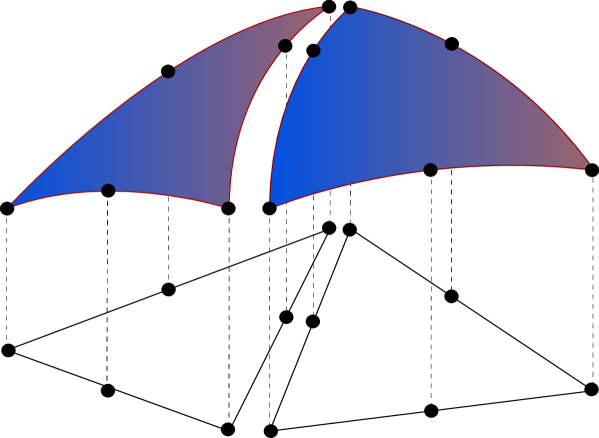
Figure 3: Piecing together local function spaces on the cells of a mesh to form a discrete function space on $\Omega$, generated by a reference finite element $(K_{0},\mathcal{P}_{0},\mathcal{N}_{0})$, a set of local-to-global mappings $\{\iota_{K}\}_{K\in\mathcal{T}}$ and a set of mappings $\{F_{K}\}_{K\in\mathcal{T}}$.

3.3 The Variational Problem

We shall assume that we are given a set of discrete function spaces defined by a corresponding set of finite elements on some triangulation $\mathcal{T}$ of a domain $\Omega\subset\mathbb{R}^{d}$. In particular, we are given a pair of function spaces,

$$\begin{split}\hat{V}_{h}&=\mathrm{span}\{\hat{\phi_{i}}\}_{i=1}^{N},\\ V_{h}&=\mathrm{span}\{\phi_{i}\}_{i=1}^{N},\end{split}$$ (28)

which we refer to as the test and trial spaces respectively.

We shall also assume that we are given a variational problem of the form: Find $U\in V_{h}$ such that

$$a(U;v)=L(v)\quad\forall v\in\hat{V}_{h},$$ (29)

where $a:V_{h}\times\hat{V}_{h}\rightarrow\mathbb{R}$ is a semilinear form which is linear in its second argument and $L:\hat{V}_{h}\rightarrow\mathbb{R}$ is a linear form (functional). Typically, the forms $a$ and $L$ of (29) are defined in terms of integrals over the domain $\Omega$ or subsets of the boundary $\partial\Omega$ of $\Omega$.

3.3.1 Nonlinear variational problems

The variational problem (29) gives rise to a system of discrete equations,

$$F(U)=0,$$ (31)

for the vector $(U_{i})\in\mathbb{R}^{N}$ of degrees of freedom of the solution $U=\sum_{i=1}^{N}U_{i}\phi_{i}\in V_{h}$, where

$$F_{i}(U)=a(U;\hat{\phi}_{i})-L(\hat{\phi}_{i}),\quad i=1,2,\ldots,N.$$ (32)

It may also be desirable to compute the Jacobian $A=F^{\prime}$ of the nonlinear system (31) for use in a Newton’s method. We note that if the semilinear form $a$ is differentiable in $U$, then the entries of the Jacobian $A$ are given by

$$\begin{split}A_{ij}&=\frac{\partial F_{i}(U)}{\partial U_{j}}=\frac{\partial}{\partial U_{j}}a(U;\hat{\phi}_{i})=a^{\prime}(U;\hat{\phi}_{i})\frac{\partial U}{\partial U_{j}}=a^{\prime}(U;\hat{\phi}_{i})\phi_{j}=a^{\prime}(U;\hat{\phi}_{i},\phi_{j}).\end{split}$$ (33)

As an example, consider the nonlinear Poisson’s equation

$$\begin{split}-\nabla\cdot((1+u)\nabla u)&=f\quad\mbox{ in }\Omega,\\ u&=0\quad\mbox{ on }\partial\Omega.\end{split}$$ (34)

Multiplying (34) with a test function $v$ and integrating by parts, we obtain

$$\int_{\Omega}\nabla v\cdot((1+u)\nabla u)\,\mathrm{d}x=\int_{\Omega}vf\,\mathrm{d}x,$$ (35)

and thus a discrete nonlinear variational problem of the form (29), where

$$\begin{split}a(U;v)&=\int_{\Omega}\nabla v\cdot((1+U)\nabla U)\,\mathrm{d}x,\\ L(v)&=\int_{\Omega}v\,f\,\mathrm{d}x.\end{split}$$ (36)

Linearizing the semilinear form $a$ around $U$, we obtain

$$a^{\prime}(U;v,w)=\int_{\Omega}\nabla v\cdot(w\nabla U)\,\mathrm{d}x+\int_{\Omega}\nabla v\cdot((1+U)\nabla w)\,\mathrm{d}x,$$ (37)

for any $w\in V_{h}$. In particular, the entries of the Jacobian matrix $A$ are given by

$$A_{ij}=a^{\prime}(U;\hat{\phi}_{i},\phi_{j})=\int_{\Omega}\nabla\hat{\phi}_{i}\cdot(\phi_{j}\nabla U)\,\mathrm{d}x+\int_{\Omega}\nabla\hat{\phi}_{i}\cdot((1+U)\nabla\phi_{j})\,\mathrm{d}x.$$ (38)

3.3.2 Linear variational problems

If the variational problem (29) is linear, the nonlinear system (31) is reduced to the linear system

$$AU=b,$$ (39)

for the degrees of freedom $(U_{i})\in\mathbb{R}^{N}$, where

$$\begin{split}A_{ij}&=a(\hat{\phi}_{i},\phi_{j}),\\ b_{i}&=L(\hat{\phi}_{i}).\end{split}$$ (40)

Note the relation to (33) in that $A_{ij}=a(\hat{\phi}_{i},\phi_{j})=a^{\prime}(U;\hat{\phi}_{i},\phi_{j})$.

In Section 2, we saw the canonical example of a linear variational problem with Poisson’s equation,

$$\begin{split}-\Delta u&=f\quad\mbox{ in }\Omega,\\ u&=0\quad\mbox{ on }\partial\Omega,\end{split}$$ (41)

corresponding to a discrete linear variational problem of the form (29), where

$$\begin{split}a(v,U)&=\int_{\Omega}\nabla v\cdot\nabla U\,\mathrm{d}x,\\ L(v)&=\int_{\Omega}v\,f\,\mathrm{d}x.\end{split}$$ (42)

3.4 Multilinear Forms

We find that for both nonlinear and linear problems, the system of discrete equations is obtained from the given variational problem by evaluating a set of multilinear forms on the set of basis functions. Noting that the semilinear form $a$ of the nonlinear variational problem (29) is a linear form for any given fixed $U\in V_{h}$ and that the form $a$ for a linear variational problem can be expressed as $a(v,U)=a^{\prime}(U;v,U)$, we thus need to be able to evaluate the following multilinear forms:

$$\begin{split}a(U;\cdot):\hat{V}_{h}\rightarrow\mathbb{R},\\ L:\hat{V}_{h}\rightarrow\mathbb{R},\\ a^{\prime}(U,\cdot,\cdot):\hat{V}_{h}\times V_{h}\rightarrow\mathbb{R}.\end{split}$$ (43)

We shall therefore consider the evaluation of general multilinear forms of arity $r>0$,

$$a:V_{h}^{1}\times V_{h}^{2}\times\cdots\times V_{h}^{r}\rightarrow\mathbb{R},$$ (44)

defined on the product space $V_{h}^{1}\times V_{h}^{2}\times\cdots\times V_{h}^{r}$ of a given set $\{V_{h}^{j}\}_{j=1}^{r}$ of discrete function spaces on a triangulation $\mathcal{T}$ of a domain $\Omega\subset\mathbb{R}^{d}$. In the simplest case, all function spaces are equal but there are many important examples, such as mixed methods, where it is important to consider arguments coming from different function spaces. We shall restrict our attention to multilinear forms expressed as integrals over the domain $\Omega$ (or subsets of its boundary).

Let now $\{\phi_{i}^{1}\}_{i=1}^{N^{1}},\{\phi_{i}^{2}\}_{i=1}^{N^{2}},\ldots,\{\phi_{i}^{r}\}_{i=1}^{N^{r}}$ be bases of $V_{h}^{1},V_{h}^{2},\ldots,V_{h}^{r}$ respectively and let $i=(i_{1},i_{2},\ldots,i_{r})$ be a multiindex of length $|i|=r$. The multilinear form $a$ then defines a rank $r$ tensor given by

$$A_{i}=a(\phi_{i_{1}}^{1},\phi_{i_{2}}^{2},\ldots,\phi_{i_{r}}^{r})\quad\forall i\in\mathcal{I},$$ (45)

where $\mathcal{I}$ is the index set

$$\mathcal{I}=\prod_{j=1}^{r}[1,|V^{j}_{h}|]=\{(1,1,\ldots,1),(1,1,\ldots,2),\ldots,(N^{1},N^{2},\ldots,N^{r})\}.$$ (46)

For any given multilinear form of arity $r$, the tensor $A$ is a (typically sparse) tensor of rank $r$ and dimension $(|V_{h}^{1}|,|V_{h}^{2}|,\ldots,|V_{h}^{r}|)=(N^{1},N^{2},\ldots,N^{r})$.

Typically, the arity of the multilinear form $a$ is $r=2$, that is, $a$ is a bilinear form, in which case the corresponding tensor $A$ is a matrix (the “stiffness matrix”), or the arity of the multilinear form $a$ is $r=1$, that is, $a$ is a linear form, in which case the corresponding tensor $A$ is a vector (“the load vector”).

Sometimes it may also be of interest to consider forms of higher arity. As an example, consider the discrete trilinear form $a:V_{h}^{1}\times V_{h}^{2}\times V_{h}^{3}\rightarrow\mathbb{R}$ associated with the weighted Poisson’s equation $-\nabla\cdot(w\nabla u)=f$. The trilinear form $a$ is given by

$$a(v,U,w)=\int_{\Omega}w\nabla v\cdot\nabla U\,\mathrm{d}x,\\$$ (47)

for $w=\sum_{i=1}^{N^{3}}w_{i}\phi_{i}^{3}\in V_{h}^{3}$ a given discrete weight function. The corresponding rank three tensor is given by

$$A_{i}=\int_{\Omega}\phi^{3}_{i_{3}}\nabla\phi^{1}_{i_{1}}\cdot\nabla\phi^{2}_{i_{2}}\,\mathrm{d}x.$$ (48)

Noting that for any $w=\sum_{i=1}^{N^{3}}w_{i}\phi_{i}^{3}$, the tensor contraction $A:w=\left(\sum_{i_{3}=1}^{N^{3}}A_{i_{1}i_{2}i_{3}}w_{i_{3}}\right)_{i_{1}i_{2}}$ is a matrix, we may thus obtain the solution $U$ by solving the linear system

$$(A:w)U=b,$$ (49)

where $b_{i}=L(\phi^{1}_{i_{1}})=\int_{\Omega}\phi^{1}_{i_{1}}f\,\mathrm{d}x$. Of course, if the solution is needed only for one single weight function $w$, it is more efficient to consider $w$ as a fixed function and directly compute the matrix $A$ associated with the bilinear form $a(\cdot,\cdot,w)$. In some cases, it may even be desirable to consider the function $U$ as being fixed and directly compute a vector $A$ (the action) associated with the linear form $a(\cdot,U,w)$, as discussed above in Section 2.1. It is thus important to consider multilinear forms of general arity $r$.

3.5 Assembling the Discrete System

The standard algorithm [121, 71, 92] for computing the tensor $A$ is known as assembly; the tensor is computed by iterating over the cells of the mesh $\mathcal{T}$ and adding from each cell the local contribution to the global tensor $A$.

To explain how the standard assembly algorithm applies to the computation of the tensor $A$ defined in (45) from a given multilinear form $a$, we note that if the multilinear form $a$ is expressed as an integral over the domain $\Omega$, we can write the multilinear form as a sum of element multilinear forms,

$$a=\sum_{K\in\mathcal{T}}a_{K},$$ (50)

and thus

$$A_{i}=\sum_{K\in\mathcal{T}}a_{K}(\phi_{i_{1}}^{1},\phi_{i_{2}}^{2},\ldots,\phi_{i_{r}}^{r}).$$ (51)

We note that in the case of Poisson’s equation, $-\Delta u=f$, the element bilinear form $a_{K}$ is given by $a_{K}(v,U)=\int_{K}\nabla v\cdot\nabla U\,\mathrm{d}x$.

We now let $\iota_{K}^{j}:[1,n_{K}^{j}]\rightarrow[1,N^{j}]$ denote the local-to-global mapping introduced above in Section 3.2 for each discrete function space $V_{h}^{j}$, $j=1,2,\ldots,r$, and define for each $K\in\mathcal{T}$ the collective local-to-global mapping $\iota_{K}:\mathcal{I}_{K}\rightarrow\mathcal{I}$ by

$$\iota_{K}(i)=(\iota_{K}^{1}(i_{1}),\iota_{K}^{2}(i_{2}),\ldots,\iota_{K}^{3}(i_{3}))\quad\forall i\in\mathcal{I}_{K},$$ (52)

where $\mathcal{I}_{K}$ is the index set

$$\mathcal{I}_{K}=\prod_{j=1}^{r}[1,|\mathcal{P}_{K}^{j}|]=\{(1,1,\ldots,1),(1,1,\ldots,2),\ldots,(n_{K}^{1},n_{K}^{2},\ldots,n_{K}^{r})\}.$$ (53)

Furthermore, for each $V_{h}^{j}$ we let $\{\phi^{K,j}_{i}\}_{i=1}^{n_{K}^{j}}$ denote the restriction to an element $K$ of the subset of the basis $\{\phi_{i}^{j}\}_{i=1}^{N^{j}}$ of $V_{h}^{j}$ supported on $K$, and for each $i\in\mathcal{I}$ we let $\mathcal{T}_{i}\subset\mathcal{T}$ denote the subset of cells on which all of the basis functions $\{\phi_{i_{j}}^{j}\}_{j=1}^{r}$ are supported.

We may now compute the tensor $A$ by summing the contributions from each local cell $K$,

$$\begin{split}A_{i}&=\sum_{K\in\mathcal{T}}a_{K}(\phi_{i_{1}}^{1},\phi_{i_{2}}^{2},\ldots,\phi_{i_{r}}^{r})=\sum_{K\in\mathcal{T}_{i}}a_{K}(\phi_{i_{1}}^{1},\phi_{i_{2}}^{2},\ldots,\phi_{i_{r}}^{r})\\ &=\sum_{K\in\mathcal{T}_{i}}a_{K}(\phi_{(\iota_{K}^{1})^{-1}(i_{1})}^{K,1},\phi_{(\iota_{K}^{2})^{-1}(i_{2})}^{K,2},\ldots,\phi_{(\iota_{K}^{r})^{-1}(i_{r})}^{K,r}).\end{split}$$ (54)

This computation may be carried out efficiently by iterating once over all cells $K\in\mathcal{T}$ and adding the contribution from each $K$ to every entry $A_{i}$ of $A$ such that $K\in\mathcal{T}_{i}$, as illustrated in Algorithm 1. In particular, we never need to form the set $\mathcal{T}_{i}$, which is implicit through the set of local-to-global mappings $\{\iota_{K}\}_{K\in\mathcal{T}}$.

$A=0$

for $K\in\mathcal{T}$

for $i\in\mathcal{I}_{K}$

$A_{\iota_{K}(i)}=A_{\iota_{K}(i)}+a_{K}(\phi_{i_{1}}^{K,1},\phi_{i_{2}}^{K,2},\ldots,\phi_{i_{r}}^{K,r})$

end for

end for

Algorithm 1 $A$ = Assemble($a$, $\{V_{h}^{j}\}_{j=1}^{r}$, $\{\iota_{K}\}_{K\in\mathcal{T}}$, $\mathcal{T}$)

The assembly algorithm may be improved by defining the element tensor $A^{K}$ by

$$A^{K}_{i}=a_{K}(\phi_{i_{1}}^{K,1},\phi_{i_{2}}^{K,2},\ldots,\phi_{i_{r}}^{K,r})\quad\forall i\in\mathcal{I}_{K}.$$ (55)

For any multilinear form of arity $r$, the element tensor $A^{K}$ is a (typically dense) tensor of rank $r$ and dimension $(n_{K}^{1},n_{K}^{2},\ldots,n_{K}^{r})$.

By computing first on each cell $K$ the element tensor $A^{K}$ before adding the entries to the tensor $A$ as in Algorithm 2, one may take advantage of optimized library routines for performing each of the two steps. Note that Algorithm 2 is independent of the algorithm used to compute the element tensor.

$A=0$

for $K\in\mathcal{T}$

Compute $A^{K}$ according to (55)

Add $A^{K}$ to $A$ according to $\iota_{K}$

end for

Algorithm 2 $A$ = Assemble($a$, $\{V_{h}^{j}\}_{j=1}^{r}$, $\{\iota_{K}\}_{K\in\mathcal{T}}$, $\mathcal{T}$)

Considering first the second operation of inserting (adding) the entries of $A^{K}$ into the global sparse tensor $A$, this may in principle be accomplished by iterating over all $i\in I_{K}$ and adding the entry $A^{K}_{i}$ at position $\iota_{K}(i)$ of $A$ as illustrated in Figure 4. However, sparse matrix libraries such as PETSc [9, 8, 10] often provide optimized routines for this type of operation, which may significantly improve the performance compared to accessing each entry of $A$ individually as in Algorithm 1. Even so, the cost of adding $A^{K}$ to $A$ may be substantial even with an efficient implementation of the sparse data structure for $A$, see [85].

\psfrag{i0}{$\iota_{K}^{1}(1)$}\psfrag{i1}{$\iota_{K}^{1}(2)$}\psfrag{i2}{$\iota_{K}^{1}(3)$}\psfrag{j0}{$\iota_{K}^{2}(1)$}\psfrag{j1}{$\iota_{K}^{2}(2)$}\psfrag{j2}{$\iota_{K}^{2}(3)$}\psfrag{A21}{$A^{K}_{32}$}\psfrag{1}{$1$}\psfrag{2}{$2$}\psfrag{3}{$3$}\includegraphics[width=341.43306pt]{eps/insertion.eps}

Figure 4: Adding the entries of the element tensor $A^{K}$ to the global tensor $A$ using the local-to-global mapping $\iota_{K}$, illustrated here for a rank two tensor (a matrix).

A similar approach can be taken to the first step of computing the element tensor, that is, an optimized library routine is called to compute the element tensor. Because of the wide variety of multilinear forms that appear in applications, a separate implementation is needed for any given multilinear form. Therefore, the implementation of this code is often left to the user, as illustrated above in Section 2.2 and Section 2.3, but the code in question may also be automatically generated and optimized for each given multilinear form. We shall return to this question below in Section 5 and Section 9.

3.6 Summary

If we thus view the finite element method as a machine that automates the discretization of differential equations, or more precisely, a machine that generates the system of discrete equations (31) from a given variational problem (29), an automation of the finite element method is straightforward up to the point of computing the element tensor for any given multilinear form and the local-to-global mapping for any given discrete function space; if the element tensor $A^{K}$ and the local-to-global mapping $\iota_{K}$ can be computed on any given cell $K$, the global tensor $A$ may be computed by Algorithm 2.

Assuming now that each of the discrete function spaces involved in the definition of the variational problem (29) is generated on some mesh $\mathcal{T}$ of the domain $\Omega$ from some reference finite element $(K_{0},\mathcal{P}_{0},\mathcal{N}_{0})$ by a set of local-to-global mappings $\{\iota_{K}\}_{K\in\mathcal{T}}$ and a set of mappings $\{F_{K}\}_{K\in\mathcal{T}}$ from the reference cell $K_{0}$, as discussed in Section 3.2, we identify the following key steps towards an automation of the finite element method:

• the automatic and efficient tabulation of the nodal basis functions on the reference finite element $(K_{0},\mathcal{P}_{0},\mathcal{N}_{0})$;

• the automatic and efficient evaluation of the element tensor $A^{K}$ on each cell $K\in\mathcal{T}$;

• the automatic and efficient assembly of the global tensor $A$ from the set of element tensors $\{A^{K}\}_{K\in\mathcal{T}}$ and the set of local-to-global mappings $\{\iota_{K}\}_{K\in\mathcal{T}}$.

We discuss each of these key steps below.

4 AUTOMATING THE TABULATION OF BASIS FUNCTIONS

Given a reference finite element $(K_{0},\mathcal{P}_{0},\mathcal{N}_{0})$, we wish to generate the unique nodal basis $\{\Phi_{i}\}_{i=1}^{n_{0}}$ for $\mathcal{P}_{0}$ satisfying

$$\nu^{0}_{i}(\Phi_{j})=\delta_{ij},\quad i,j=1,2,\ldots,n_{0}.$$ (56)

In some simple cases, these nodal basis functions can be worked out analytically by hand or found in the literature, see for example [121, 71]. As a concrete example, consider the nodal basis functions in the case when $\mathcal{P}_{0}$ is the set of quadratic polynomials on the reference triangle $K_{0}$ with vertices at $v^{1}=(0,0)$, $v^{2}=(1,0)$ and $v^{3}=(0,1)$ as in Figure 5 and nodes $\mathcal{N}_{0}=\{\nu^{0}_{1},\nu^{0}_{2},\ldots,\nu^{0}_{6}\}$ given by point evaluation at the vertices and edge midpoints. A basis for $\mathcal{P}_{0}$ is then given by

$$\begin{split}\Phi_{1}(X)&=(1-X_{1}-X_{2})(1-2X_{1}-2X_{2}),\\ \Phi_{2}(X)&=X_{1}(2X_{1}-1),\\ \Phi_{3}(X)&=X_{2}(2X_{2}-1),\\ \Phi_{4}(X)&=4X_{1}X_{2},\\ \Phi_{5}(X)&=4X_{2}(1-X_{1}-X_{2}),\\ \Phi_{6}(X)&=4X_{1}(1-X_{1}-X_{2}),\end{split}$$ (57)

and it is easy to verify that this is the nodal basis. However, in the general case, it may be very difficult to obtain analytical expressions for the nodal basis functions. Furthermore, copying the often complicated analytical expressions into a computer program is prone to errors and may even result in inefficient code.

\psfrag{p0}{}\psfrag{p1}{}\psfrag{p2}{}\psfrag{p3}{}\psfrag{v0}{$v^{1}$}\psfrag{v1}{$v^{2}$}\psfrag{v2}{$v^{3}$}\psfrag{v3}{$v^{4}$}\psfrag{x0}{$X_{1}$}\psfrag{x1}{$X_{2}$}\psfrag{x2}{$X_{3}$}\includegraphics[width=193.47882pt]{eps/reference_triangle.eps}

\psfrag{p0}{}\psfrag{p1}{}\psfrag{p2}{}\psfrag{p3}{}\psfrag{v0}{$v^{1}$}\psfrag{v1}{$v^{2}$}\psfrag{v2}{$v^{3}$}\psfrag{v3}{$v^{4}$}\psfrag{x0}{$X_{1}$}\psfrag{x1}{$X_{2}$}\psfrag{x2}{$X_{3}$}\includegraphics[width=193.47882pt]{eps/reference_tetrahedron.eps}

Figure 5: The reference triangle (left) with vertices at $v^{1}=(0,0)$, $v^{2}=(1,0)$ and $v^{3}=(0,1)$, and the reference tetrahedron (right) with vertices at $v^{1}=(0,0,0)$, $v^{2}=(1,0,0)$, $v^{3}=(0,1,0)$ and $v^{4}=(0,0,1)$.

In recent work, Kirby [83, 82, 84] has proposed a solution to this problem; by expanding the nodal basis functions for $\mathcal{P}_{0}$ as linear combinations of another (non-nodal) basis for $\mathcal{P}_{0}$ which is easy to compute, one may translate operations on the nodal basis functions, such as evaluation and differentiation, into linear algebra operations on the expansion coefficients.

This new linear algebraic approach to computing and representing finite element basis functions removes the need for having explicit expressions for the nodal basis functions, thus simplifying or enabling the implementation of complicated finite elements.

4.1 Tabulating Polynomial Spaces

To generate the set of nodal basis functions $\{\Phi_{i}\}_{i=1}^{n_{0}}$ for $\mathcal{P}_{0}$, we must first identify some other known basis $\{\Psi_{i}\}_{i=1}^{n_{0}}$ for $\mathcal{P}_{0}$, referred to in [82] as the prime basis. We return to the question of how to choose the prime basis below.

Writing now each $\Phi_{i}$ as a linear combination of the prime basis functions with $\alpha\in\mathbb{R}^{d\times d}$ the matrix of coefficients, we have

$$\Phi_{i}=\sum_{j=1}^{n_{0}}\alpha_{ij}\Psi_{j},\quad i=1,2,\ldots,n_{0}.$$ (58)

The conditions (56) thus translate into

$$\delta_{ij}=\nu^{0}_{i}(\Phi_{j})=\sum_{k=1}^{n_{0}}\alpha_{jk}\nu^{0}_{i}(\Psi_{k}),\quad i,j=1,2,\ldots,n_{0},$$ (59)

or

$$\mathcal{V}\alpha^{\top}=I,$$ (60)

where $\mathcal{V}\in\mathbb{R}^{n_{0}\times n_{0}}$ is the (Vandermonde) matrix with entries $\mathcal{V}_{ij}=\nu^{0}_{i}(\Psi_{j})$ and $I$ is the $n_{0}\times n_{0}$ identity matrix. Thus, the nodal basis $\{\Phi_{i}\}_{i=1}^{n_{0}}$ is easily computed by first computing the matrix $\mathcal{V}$ by evaluating the nodes at the prime basis functions and then solving the linear system (60) to obtain the matrix $\alpha$ of coefficients.

In the simplest case, the space $\mathcal{P}_{0}$ is the set $P_{q}(K_{0})$ of polynomials of degree $\leq q$ on $K_{0}$. For typical reference cells, including the reference triangle and the reference tetrahedron shown in Figure 5, orthogonal prime bases are available with simple recurrence relations for the evaluation of the basis functions and their derivatives, see for example [33]. If $\mathcal{P}_{0}=P_{q}(K_{0})$, it is thus straightforward to evaluate the prime basis and thus to generate and solve the linear system $(\ref{eq:fiatsystem})$ that determines the nodal basis.

4.2 Tabulating Spaces with Constraints

In other cases, the space $\mathcal{P}_{0}$ may be defined as some subspace of $P_{q}(K_{0})$, typically by constraining certain derivatives of the functions in $\mathcal{P}_{0}$ or the functions themselves to lie in $P_{q^{\prime}}(K_{0})$ for some $q^{\prime}<q$ on some part of $K_{0}$. Examples include the the Raviart–Thomas [111], Brezzi–Douglas–Fortin–Marini [23] and Arnold–Winther [4] elements, which put constraints on the derivatives of the functions in $\mathcal{P}_{0}$.

Another more obvious example, taken from [82], is the case when the functions in $\mathcal{P}_{0}$ are constrained to $P_{q-1}(\gamma_{0})$ on some part $\gamma_{0}$ of the boundary of $K_{0}$ but are otherwise in $P_{q}(K_{0})$, which may be used to construct the function space on a $p$-refined cell $K$ if the function space on a neighboring cell $K^{\prime}$ with common boundary $\gamma_{0}$ is only $P_{q-1}(K^{\prime})$. We may then define the space $\mathcal{P}_{0}$ by

$$\mathcal{P}_{0}=\{v\in P_{q}(K_{0}):v|_{\gamma_{0}}\in P_{q-1}(\gamma_{0})\}=\{v\in P_{q}(K_{0}):l(v)=0\},$$ (61)

where the linear functional $l$ is given by integration against the $q$th degree Legendre polynomial along the boundary $\gamma_{0}$.

In general, one may define a set $\{l_{i}\}_{i=1}^{n_{c}}$ of linear functionals (constraints) and define $\mathcal{P}_{0}$ as the intersection of the null spaces of these linear functionals on $P_{q}(K_{0})$,

$$\mathcal{P}_{0}=\{v\in P_{q}(K_{0}):l_{i}(v)=0,\quad i=1,2,\ldots,n_{c}\}.$$ (62)

To find a prime basis $\{\Psi_{i}\}_{i=1}^{n_{0}}$ for $\mathcal{P}_{0}$, we note that any function in $\mathcal{P}_{0}$ may be expressed as a linear combination of some basis functions $\{\bar{\Psi}_{i}\}_{i=1}^{|P_{q}(K_{0})|}$ for $P_{q}(K_{0})$, which we may take as the orthogonal basis discussed above. We find that if $\Psi=\sum_{i=1}^{|P_{q}(K_{0})|}\beta_{i}\bar{\Psi}_{i}$, then

$$0=l_{i}(\Psi)=\sum_{j=1}^{|P_{q}(K_{0})|}\beta_{j}l_{i}(\bar{\Psi}_{j}),\quad i=1,2,\ldots,n_{c},$$ (63)

or

$$L\beta=0,$$ (64)

where $L$ is the $n_{c}\times|P_{q}(K_{0})|$ matrix with entries

$$L_{ij}=l_{i}(\bar{\Psi}_{j}),\quad i=1,2,\ldots,n_{c},\quad j=1,2,\ldots,|P_{q}(K_{0})|.$$ (65)

A prime basis for $\mathcal{P}_{0}$ may thus be found by computing the nullspace of the matrix $L$, for example by computing its singular value decomposition (see [58]). Having thus found the prime basis $\{\Psi_{i}\}_{i=1}^{n_{0}}$, we may proceed to compute the nodal basis as before.

5 AUTOMATING THE COMPUTATION OF THE ELEMENT TENSOR

As we saw in Section 3.5, given a multilinear form $a$ defined on the product space $V_{h}^{1}\times V_{h}^{2}\times\ldots\times V_{h}^{r}$, we need to compute for each cell $K\in\mathcal{T}$ the rank $r$ element tensor $A^{K}$ given by

$$A^{K}_{i}=a_{K}(\phi_{i_{1}}^{K,1},\phi_{i_{2}}^{K,2},\ldots,\phi_{i_{r}}^{K,r})\quad\forall i\in\mathcal{I}_{K},$$ (66)

where $a_{K}$ is the local contribution to the multilinear form $a$ from the cell $K$.

We investigate below two very different ways to compute the element tensor, first a modification of the standard approach based on quadrature and then a novel approach based on a special tensor contraction representation of the element tensor, yielding speedups of several orders of magnitude in some cases.

5.1 Evaluation by Quadrature

The element tensor $A^{K}$ is typically evaluated by quadrature on the cell $K$. Many finite element libraries like Diffpack [24, 92] and deal.II [12, 13, 11] provide the values of relevant quantities like basis functions and their derivatives at the quadrature points on $K$ by mapping precomputed values of the corresponding basis functions on the reference cell $K_{0}$ using the mapping $F_{K}:K_{0}\rightarrow K$.

Thus, to evaluate the element tensor $A^{K}$ for Poisson’s equation by quadrature on $K$, one computes

$$A^{K}_{i}=\int_{K}\nabla\phi_{i_{1}}^{K,1}\cdot\nabla\phi_{i_{2}}^{K,2}\,\mathrm{d}x\approx\sum_{k=1}^{N_{q}}w_{k}\nabla\phi_{i_{1}}^{K,1}(x^{k})\cdot\nabla\phi_{i_{2}}^{K,2}(x^{k})\det F_{K}^{\prime}(x^{k}),$$ (67)

for some suitable set of quadrature points $\{x^{i}\}_{i=1}^{N_{q}}\subset K$ with corresponding quadrature weights $\{w_{i}\}_{i=1}^{N_{q}}$, where we assume that the quadrature weights are scaled so that $\sum_{i=1}^{N_{q}}w_{i}=|K_{0}|$. Note that the approximation (67) can be made exact for a suitable choice of quadrature points if the basis functions are polynomials.

Comparing (67) to the example codes in Table 3 and Table 4, we note the similarities between (67) and the two codes. In both cases, the gradients of the basis functions as well as the products of quadrature weight and the determinant of $F_{K}^{\prime}$ are precomputed at the set of quadrature points and then combined to produce the integral (67).

If we assume that the two discrete spaces $V_{h}^{1}$ and $V_{h}^{2}$ are equal, so that the local basis functions $\{\phi^{K,1}_{i}\}_{i=1}^{n_{K}^{1}}$ and $\{\phi^{K,2}_{i}\}_{i=1}^{n_{K}^{2}}$ are all generated from the same basis $\{\Phi_{i}\}_{i=1}^{n_{0}}$ on the reference cell $K_{0}$, the work involved in precomputing the gradients of the basis functions at the set of quadrature points amounts to computing for each quadrature point $x_{k}$ and each basis function $\phi^{K}_{i}$ the matrix–vector product $\nabla_{x}\phi^{K}_{i}(x_{k})=(F_{K}^{\prime})^{-\top}(x_{k})\nabla_{X}\Phi_{i}(X_{k})$, that is,

$$\frac{\partial\phi^{K}_{i}}{\partial x_{j}}(x^{k})=\sum_{l=1}^{d}\frac{\partial X_{l}}{\partial x_{j}}(x^{k})\frac{\partial\Phi^{K}_{i}}{\partial X_{l}}(X^{k}),$$ (68)

where $x^{k}=F_{K}(X^{k})$ and $\phi^{K}_{i}=\Phi_{i}\circ F_{K}^{-1}$. Note that the the gradients $\{\nabla_{X}\Phi_{i}(X_{k})\}_{i=1,k=1}^{n_{0},N_{q}}$ of the reference element basis functions at the set of quadrature points on the reference element remain constant throughout the assembly process and may be pretabulated and stored. Thus, the gradients of the basis functions on $K$ may be computed in $N_{q}n_{0}d^{2}$ multiply–add pairs (MAPs) and the total work to compute the element tensor $A^{K}$ is $N_{q}n_{0}d^{2}+N_{q}n_{0}^{2}(d+2)\sim N_{q}n_{0}^{2}d$, if we ignore that we also need to compute the mapping $F_{K}$, and the determinant and inverse of $F_{K}^{\prime}$. In Section 5.2 and Section 7 below, we will see that this operation count may be significantly reduced.

5.2 Evaluation by Tensor Representation

It has long been known that it is sometimes possible to speed up the computation of the element tensor by precomputing certain integrals on the reference element. Thus, for any specific multilinear form, it may be possible to find quantities that can be precomputed in order to optimize the code for the evaluation of the element tensor. These ideas were first introduced in a general setting in [85, 86] and later formalized and automated in [87, 88]. A similar approach was implemented in early versions of DOLFIN [62, 68, 63], but only for piecewise linear elements.

We first consider the case when the mapping $F_{K}$ from the reference cell is affine, and then discuss possible extensions to non-affine mappings such as when $F_{K}$ is the isoparametric mapping. As a first example, we consider again the computation of the element tensor $A^{K}$ for Poisson’s equation. As before, we have

$$A^{K}_{i}=\int_{K}\nabla\phi_{i_{1}}^{K,1}\cdot\nabla\phi_{i_{2}}^{K,2}\,\mathrm{d}x=\int_{K}\sum_{\beta=1}^{d}\frac{\partial\phi_{i_{1}}^{K,1}}{\partial x_{\beta}}\frac{\partial\phi_{i_{2}}^{K,2}}{\partial x_{\beta}}\,\mathrm{d}x,$$ (69)

but instead of evaluating the gradients on $K$ and then proceeding to evaluate the integral by quadrature, we make a change of variables to write

$$A^{K}_{i}=\int_{K_{0}}\sum_{\beta=1}^{d}\sum_{\alpha_{1}=1}^{d}\frac{\partial X_{\alpha_{1}}}{\partial x_{\beta}}\frac{\partial\Phi^{1}_{i_{1}}}{\partial X_{\alpha_{1}}}\sum_{\alpha_{2}=1}^{d}\frac{\partial X_{\alpha_{2}}}{\partial x_{\beta}}\frac{\partial\Phi^{2}_{i_{2}}}{\partial X_{\alpha_{2}}}\det F_{K}^{\prime}\,\mathrm{d}X,$$ (70)

and thus, if the mapping $F_{K}$ is affine so that the transforms $\partial X/\partial x$ and the determinant $\det F_{K}^{\prime}$ are constant, we obtain

$$A^{K}_{i}=\det F_{K}^{\prime}\sum_{\alpha_{1}=1}^{d}\sum_{\alpha_{2}=1}^{d}\sum_{\beta=1}^{d}\frac{\partial X_{\alpha_{1}}}{\partial x_{\beta}}\frac{\partial X_{\alpha_{2}}}{\partial x_{\beta}}\int_{K_{0}}\frac{\partial\Phi^{1}_{i_{1}}}{\partial X_{\alpha_{1}}}\frac{\partial\Phi^{2}_{i_{2}}}{\partial X_{\alpha_{2}}}\,\mathrm{d}X=\sum_{\alpha_{1}=1}^{d}\sum_{\alpha_{2}=1}^{d}A^{0}_{i\alpha}G_{K}^{\alpha},$$ (71)

or

$$A^{K}=A^{0}:G_{K},$$ (72)

where

$$\begin{split}A^{0}_{i\alpha}&=\int_{K_{0}}\frac{\partial\Phi^{1}_{i_{1}}}{\partial X_{\alpha_{1}}}\frac{\partial\Phi^{2}_{i_{2}}}{\partial X_{\alpha_{2}}}\,\mathrm{d}X,\\ G_{K}^{\alpha}&=\det F_{K}^{\prime}\sum_{\beta=1}^{d}\frac{\partial X_{\alpha_{1}}}{\partial x_{\beta}}\frac{\partial X_{\alpha_{2}}}{\partial x_{\beta}}.\end{split}$$ (73)

We refer to the tensor $A^{0}$ as the reference tensor and to the tensor $G_{K}$ as the geometry tensor.

Now, since the reference tensor is constant and does not depend on the cell $K$, it may be precomputed before the assembly of the global tensor $A$. For the current example, the work on each cell $K$ thus involves first computing the rank two geometry tensor $G^{K}$, which may be done in $d^{3}$ multiply–add pairs, and then computing the rank two element tensor $A^{K}$ as the tensor contraction (72), which may be done in $n_{0}^{2}d^{2}$ multiply–add pairs. Thus, the total operation count is $d^{3}+n_{0}^{2}d^{2}\sim n_{0}^{2}d^{2}$, which should be compared to $N_{q}n_{0}^{2}d$ for the standard quadrature-based approach. The speedup in this particular case is thus roughly a factor $N_{q}/d$, which may be a significant speedup, in particular for higher order elements.

As we shall see, the tensor representation (72) generalizes to other multilinear forms as well. To see this, we need to make some assumptions about the structure of the multilinear form (44). We shall assume that the multilinear form $a$ is expressed as an integral over $\Omega$ of a weighted sum of products of basis functions or derivatives of basis functions. In particular, we shall assume that the element tensor $A^{K}$ can be expressed as a sum, where each term takes the following canonical form,

$$A^{K}_{i}=\sum_{\gamma\in\mathcal{C}}\int_{K}\prod_{j=1}^{m}c_{j}(\gamma)D_{x}^{\delta_{j}(\gamma)}\phi^{K,j}_{\iota_{j}(i,\gamma)}[\kappa_{j}(\gamma)]\,\mathrm{d}x,$$ (74)

where $\mathcal{C}$ is some given set of multiindices, each coefficient $c_{j}$ maps the multiindex $\gamma$ to a real number, $\iota_{j}$ maps $(i,\gamma)$ to a basis function index, $\kappa_{j}$ maps $\gamma$ to a component index (for vector or tensor valued basis functions) and $\delta_{j}$ maps $\gamma$ to a derivative multiindex. To distinguish component indices from indices for basis functions, we use $[\cdot]$ to denote a component index and subscript to denote a basis function index. In the simplest case, the number of factors $m$ is equal to the arity $r$ of the multilinear form (rank of the tensor), but in general, the canonical form (74) may contain factors that correspond to additional functions which are not arguments of the multilinear form. This is the case for the weighted Poisson’s equation (47), where $m=3$ and $r=2$. In general, we thus have $m>r$.

As an illustration of this notation, we consider again the bilinear form for Poisson’s equation and write it in the notation of (74). We will also consider a more involved example to illustrate the generality of the notation. From (69), we have

$$A^{K}_{i}=\int_{K}\sum_{\gamma=1}^{d}\frac{\partial\phi_{i_{1}}^{K,1}}{\partial x_{\gamma}}\frac{\partial\phi_{i_{2}}^{K,2}}{\partial x_{\gamma}}\,\mathrm{d}x=\sum_{\gamma=1}^{d}\int_{K}\frac{\partial\phi_{i_{1}}^{K,1}}{\partial x_{\gamma}}\frac{\partial\phi_{i_{2}}^{K,2}}{\partial x_{\gamma}}\,\mathrm{d}x,$$ (75)

and thus, in the notation of (74),

$$\begin{split}m&=2,\\ \mathcal{C}&=[1,d],\\ c(\gamma)&=(1,1),\\ \iota(i,\gamma)&=(i_{1},i_{2}),\\ \kappa(\gamma)&=(\emptyset,\emptyset),\\ \delta(\gamma)&=(\gamma,\gamma),\end{split}$$ (76)

where $\emptyset$ denotes an empty component index (the basis functions are scalar).

As another example, we consider the bilinear form for a stabilization term appearing in a least-squares stabilized $\mathrm{cG}(1)\mathrm{cG}(1)$ method for the incompressible Navier–Stokes equations [40, 65, 64, 66],

$$a(v,U)=\int_{\Omega}(w\cdot\nabla v)\cdot(w\cdot\nabla U)\,\mathrm{d}x=\int_{\Omega}\sum_{\gamma_{1},\gamma_{2},\gamma_{3}=1}^{d}w[\gamma_{2}]\frac{\partial v[\gamma_{1}]}{\partial x_{\gamma_{2}}}w[\gamma_{3}]\frac{\partial U[\gamma_{1}]}{\partial x_{\gamma_{3}}}\,\mathrm{d}x,$$ (77)

where $w\in V_{h}^{3}=V_{h}^{4}$ is a given approximation of the velocity, typically obtained from the previous iteration in an iterative method for the nonlinear Navier–Stokes equations. To write the element tensor for (77) in the canonical form (74), we expand $w$ in the nodal basis for $\mathcal{P}_{K}^{3}=\mathcal{P}_{K}^{4}$ and note that

$$A^{K}_{i}=\sum_{\gamma_{1},\gamma_{2},\gamma_{3}=1}^{d}\sum_{\gamma_{4}=1}^{n_{K}^{3}}\sum_{\gamma_{5}=1}^{n_{K}^{4}}\int_{K}\frac{\partial\phi^{K,1}_{i_{1}}[\gamma_{1}]}{\partial x_{\gamma_{2}}}\frac{\partial\phi^{K,2}_{i_{2}}[\gamma_{1}]}{\partial x_{\gamma_{3}}}w_{\gamma_{4}}^{K}\phi^{K,3}_{\gamma_{4}}[\gamma_{2}]w_{\gamma_{5}}^{K}\phi^{K,4}_{\gamma_{5}}[\gamma_{3}]\,\mathrm{d}x,$$ (78)

We may then write the element tensor $A^{K}$ for the bilinear form (77) in the canonical form (74), with

$$\begin{split}m&=4,\\ \mathcal{C}&=[1,d]^{3}\times[1,n_{K}^{3}]\times[1,n_{K}^{4}],\\ c(\gamma)&=(1,1,w_{\gamma_{4}}^{K},w_{\gamma_{5}}^{K}),\\ \iota(i,\gamma)&=(i_{1},i_{2},\gamma_{4},\gamma_{5}),\\ \kappa(\gamma)&=(\gamma_{1},\gamma_{1},\gamma_{2},\gamma_{3}),\\ \delta(\gamma)&=(\gamma_{2},\gamma_{3},\emptyset,\emptyset),\end{split}$$ (79)

where $\emptyset$ denotes an empty derivative multiindex (no differentiation).

In [88], it is proved that any element tensor $A^{K}$ that can be expressed in the general canonical form (74), can be represented as a tensor contraction $A^{K}=A^{0}:G_{K}$ of a reference tensor $A^{0}$ independent of $K$ and a geometry tensor $G_{K}$. A similar result is also presented in [87] but in less formal notation. As noted above, element tensors that can be expressed in the general canonical form correspond to multilinear forms that can be expressed as integrals over $\Omega$ of linear combinations of products of basis functions and their derivatives. The representation theorem reads as follows.

Theorem 1 (Representation theorem)

If $F_{K}$ is a given affine mapping from a reference cell $K_{0}$ to a cell $K$ and $\{\mathcal{P}_{K}^{j}\}_{j=1}^{m}$ is a given set of discrete function spaces on $K$, each generated by a discrete function space $\mathcal{P}_{0}^{j}$ on the reference cell $K_{0}$ through the affine mapping, that is, for each $\phi\in\mathcal{P}_{K}^{j}$ there is some $\Phi\in\mathcal{P}_{0}^{j}$ such that $\Phi=\phi\circ F_{K}$, then the element tensor (74) may be represented as the tensor contraction of a reference tensor $A^{0}$ and a geometry tensor $G_{K}$,

$$A^{K}=A^{0}:G_{K},$$ (80)

that is,

$$A^{K}_{i}=\sum_{\alpha\in\mathcal{A}}A^{0}_{i\alpha}G_{K}^{\alpha}\quad\forall i\in\mathcal{I}_{K},$$ (81)

where the reference tensor $A^{0}$ is independent of $K$. In particular, the reference tensor $A^{0}$ is given by

$$A^{0}_{i\alpha}=\sum_{\beta\in\mathcal{B}}\int_{K_{0}}\prod_{j=1}^{m}D_{X}^{\delta^{\prime}_{j}(\alpha,\beta)}\Phi^{j}_{\iota_{j}(i,\alpha,\beta)}[\kappa_{j}(\alpha,\beta)]\,\mathrm{d}X,$$ (82)

and the geometry tensor $G_{K}$ is the outer product of the coefficients of any weight functions with a tensor that depends only on the Jacobian $F_{K}^{\prime}$,

$$G_{K}^{\alpha}=\prod_{j=1}^{m}c_{j}(\alpha)\,\det F_{K}^{\prime}\sum_{\beta\in\mathcal{B^{\prime}}}\prod_{j^{\prime}=1}^{m}\prod_{k=1}^{|\delta_{j^{\prime}}(\alpha,\beta)|}\frac{\partial X_{\delta^{\prime}_{j^{\prime}k}(\alpha,\beta)}}{\partial x_{\delta_{j^{\prime}k}(\alpha,\beta)}},$$ (83)

for some appropriate index sets $\mathcal{A}$, $\mathcal{B}$ and $\mathcal{B}^{\prime}$. We refer to the index set $\mathcal{I}_{K}$ as the set of primary indices, the index set $\mathcal{A}$ as the set of secondary indices, and to the index sets $\mathcal{B}$ and $\mathcal{B}^{\prime}$ as sets of auxiliary indices.

The ranks of the tensors $A^{0}$ and $G_{K}$ are determined by the properties of the multilinear form $a$, such as the number of coefficients and derivatives. Since the rank of the element tensor $A^{K}$ is equal to the arity $r$ of the multilinear form $a$, the rank of the reference tensor $A^{0}$ must be $|i\alpha|=r+|\alpha|$, where $|\alpha|$ is the rank of the geometry tensor. For the examples presented above, we have $|i\alpha|=4$ and $|\alpha|=2$ in the case of Poisson’s equation and $|i\alpha|=8$ and $|\alpha|=6$ for the Navier–Stokes stabilization term.

The proof of Theorem 1 is constructive and gives an algorithm for computing the representation (80). A number of concrete examples with explicit formulas for the reference and geometry tensors are given in Tables 10–13. We return to these test cases below in Section 9.2, when we discuss the implementation of Theorem 1 in the form compiler FFC and present benchmark results for the test cases.

We remark that in general, a multilinear form will correspond to a sum of tensor contractions, rather than a single tensor contraction as in (80), that is,

$$A^{K}=\sum_{k}A^{0,k}:G_{K,k}.$$ (84)

One such example is the computation of the element tensor for the convection–reaction problem $-\Delta u+u=f$, which may be computed as the sum of a tensor contraction of a rank four reference tensor $A^{0,1}$ with a rank two geometry tensor $G_{K,1}$ and a rank two reference tensor $A^{0,2}$ with a rank zero geometry tensor $G_{K,2}$.

$a(v,U)$	$=$	$\int_{\Omega}v\,U\,\mathrm{d}x$	rank
$A^{0}_{i\alpha}$	$=$	$\int_{K_{0}}\Phi_{i_{1}}^{1}\Phi_{i_{2}}^{2}\,\mathrm{d}X$	$|i\alpha|=2$
$G_{K}^{\alpha}$	$=$	$\det F_{K}^{\prime}$	$|\alpha|=0$

Table 10: The tensor contraction representation $A^{K}=A^{0}:G_{K}$ of the element tensor $A^{K}$ for the bilinear form associated with a mass matrix (test case 1).

$a(v,U)$	$=$	$\int_{\Omega}\nabla v\cdot\nabla U\,\mathrm{d}x$	rank
$A^{0}_{i\alpha}$	$=$	$\int_{K_{0}}\frac{\partial\Phi^{1}_{i_{1}}}{\partial X_{\alpha_{1}}}\frac{\partial\Phi^{2}_{i_{2}}}{\partial X_{\alpha_{2}}}\,\mathrm{d}X$	$|i\alpha|=4$
$G_{K}^{\alpha}$	$=$	$\det F_{K}^{\prime}\sum_{\beta=1}^{d}\frac{\partial X_{\alpha_{1}}}{\partial x_{\beta}}\frac{\partial X_{\alpha_{2}}}{\partial x_{\beta}}$	$|\alpha|=2$

Table 11: The tensor contraction representation $A^{K}=A^{0}:G_{K}$ of the element tensor $A^{K}$ for the bilinear form associated with Poisson’s equation (test case 2).

$a(v,U)$	$=$	$\int_{\Omega}v\cdot(w\cdot\nabla)U\,\mathrm{d}x$	rank
$A^{0}_{i\alpha}$	$=$	$\sum_{\beta=1}^{d}\int_{K_{0}}\Phi^{1}_{i_{1}}[\beta]\frac{\partial\Phi^{2}_{i_{2}}[\beta]}{\partial X_{\alpha_{3}}}\Phi^{3}_{\alpha_{1}}[\alpha_{2}]\,\mathrm{d}X$	$|i\alpha|=5$
$G_{K}^{\alpha}$	$=$	$w^{K}_{\alpha_{1}}\det F_{K}^{\prime}\frac{\partial X_{\alpha_{3}}}{\partial x_{\alpha_{2}}}$	$|\alpha|=3$

Table 12: The tensor contraction representation $A^{K}=A^{0}:G_{K}$ of the element tensor $A^{K}$ for the bilinear form associated with a linearization of the nonlinear term $u\cdot\nabla u$ in the incompressible Navier–Stokes equations (test case 3).

$a(v,U)$	$=$	$\int_{\Omega}\epsilon(v):\epsilon(U)\,\mathrm{d}x$	rank
$A^{0}_{i\alpha}$	$=$	$\sum_{\beta=1}^{d}\int_{K_{0}}\frac{\partial\Phi^{1}_{i_{1}}[\beta]}{\partial X_{\alpha_{1}}}\frac{\partial\Phi^{2}_{i_{2}}[\beta]}{\partial X_{\alpha_{2}}}\,\mathrm{d}X$	$|i\alpha|=4$
$G_{K}^{\alpha}$	$=$	$\frac{1}{2}\det F_{K}^{\prime}\sum_{\beta=1}^{d}\frac{\partial X_{\alpha_{1}}}{\partial x_{\beta}}\frac{\partial X_{\alpha_{2}}}{\partial x_{\beta}}$	$|\alpha|=2$

Table 13: The tensor contraction representation $A^{K}=A^{0}:G_{K}$ of the element tensor $A^{K}$ for the bilinear form $\int_{\Omega}\epsilon(v):\epsilon(U)\,\mathrm{d}x=\int_{\Omega}\frac{1}{4}(\nabla v+(\nabla v)^{\top}):(\nabla U+(\nabla U)^{\top})\,\mathrm{d}x$ associated with the strain-strain term of linear elasticity (test case 4). Note that the product expands into four terms which can be grouped in pairs of two. The representation is given only for the first of these two terms.

5.3 Extension to Non-Affine Mappings

The tensor contraction representation (80) of Theorem 1 assumes that the mapping $F_{K}$ from the reference cell is affine, allowing the transforms $\partial X/\partial x$ and the determinant to be pulled out of the integral. To see how to extend this result to the case when the mapping $F_{K}$ is non-affine, such as in the case of an isoparametric mapping for a higher-order element used to map the reference cell to a curvilinear cell on the boundary of $\Omega$, we consider again the computation of the element tensor $A^{K}$ for Poisson’s equation. As in Section 5.1, we use quadrature to evaluate the integral, but take advantage of the fact that the discrete function spaces $\mathcal{P}_{K}^{1}$ and $\mathcal{P}_{K}^{2}$ on $K$ may be generated from a pair of reference finite elements as discussed in Section 3.2. We have

$$\begin{split}A^{K}_{i}&=\int_{K}\nabla\phi_{i_{1}}^{K,1}\cdot\nabla\phi_{i_{2}}^{K,2}\,\mathrm{d}x=\int_{K}\sum_{\beta=1}^{d}\frac{\partial\phi_{i_{1}}^{K,1}}{\partial x_{\beta}}\frac{\partial\phi_{i_{2}}^{K,2}}{\partial x_{\beta}}\,\mathrm{d}x\\ &=\sum_{\alpha_{1}=1}^{d}\sum_{\alpha_{2}=1}^{d}\sum_{\beta=1}^{d}\ \int_{K_{0}}\frac{\partial X_{\alpha_{1}}}{\partial x_{\beta}}\frac{\partial X_{\alpha_{2}}}{\partial x_{\beta}}\frac{\partial\Phi_{i_{1}}^{1}}{\partial X_{\alpha_{1}}}\frac{\partial\Phi_{i_{2}}^{2}}{\partial X_{\alpha_{2}}}\det F_{K}^{\prime}\,\mathrm{d}X\\ &\approx\sum_{\alpha_{1}=1}^{d}\sum_{\alpha_{2}=1}^{d}\sum_{\alpha_{3}=1}^{N_{q}}w_{\alpha_{3}}\frac{\partial\Phi_{i_{1}}^{1}}{\partial X_{\alpha_{1}}}(X_{\alpha_{3}})\frac{\partial\Phi_{i_{2}}^{2}}{\partial X_{\alpha_{2}}}(X_{\alpha_{3}})\sum_{\beta=1}^{d}\frac{\partial X_{\alpha_{1}}}{\partial x_{\beta}}(X_{\alpha_{3}})\frac{\partial X_{\alpha_{2}}}{\partial x_{\beta}}(X_{\alpha_{3}})\det F_{K}^{\prime}(X_{\alpha_{3}}).\end{split}$$ (85)

As before, we thus obtain a representation of the form

$$A^{K}=A^{0}:G_{K},$$ (86)

where the reference tensor $A^{0}$ is now given by

$$A^{0}_{i\alpha}=w_{\alpha_{3}}\frac{\partial\Phi_{i_{1}}^{1}}{\partial X_{\alpha_{1}}}(X_{\alpha_{3}})\frac{\partial\Phi_{i_{2}}^{2}}{\partial X_{\alpha_{2}}}(X_{\alpha_{3}}),$$ (87)

and the geometry tensor $G_{K}$ is given by

$$G_{K}^{\alpha}=\det F_{K}^{\prime}(X_{\alpha_{3}})\sum_{\beta=1}^{d}\frac{\partial X_{\alpha_{1}}}{\partial x_{\beta}}(X_{\alpha_{3}})\frac{\partial X_{\alpha_{2}}}{\partial x_{\beta}}(X_{\alpha_{3}}).$$ (88)

We thus note that a (different) tensor contraction representation of the element tensor $A^{K}$ is possible even if the mapping $F_{K}$ is non-affine. One may also prove a representation theorem similar to Theorem 1 for non-affine mappings.

Comparing the representation (87)–(88) with the affine representation (73), we note that the ranks of both $A^{0}$ and $G_{K}$ have increased by one. As before, we may precompute the reference tensor $A^{0}$ but the number of multiply–add pairs to compute the element tensor $A^{K}$ increase by a factor $N_{q}$ from $n_{0}^{2}d^{2}$ to $N_{q}n_{0}^{2}d^{2}$ (if again we ignore the cost of computing the geometry tensor).

We also note that the cost has increased by a factor $d$ compared to the cost of a direct application of quadrature as described in Section 5.1. However, by expressing the element tensor $A^{K}$ as a tensor contraction, the evaluation of the element tensor is more readily optimized than if expressed as a triply nested loop over quadrature points and basis functions as in Table 3 and Table 4.

As demonstrated below in Section 7, it may in some cases be possible to take advantage of special structures such as dependencies between different entries in the tensor $A^{0}$ to significantly reduce the operation count. Another more straightforward approach is to use an optimized library routine such as a BLAS call to compute the tensor contraction as we shall see below in Section 7.1.

5.4 A Language for Multilinear Forms

To automate the process of evaluating the element tensor $A^{K}$, we must create a system that takes as input a multilinear form $a$ and automatically computes the corresponding element tensor $A^{K}$. We do this by defining a language for multilinear forms and automatically translating any given string in the language to the canonical form (74). From the canonical form, we may then compute the element tensor $A^{K}$ by the tensor contraction $A^{K}=A^{0}:G_{K}$.

When designing such a language for multilinear forms, we have two things in mind. First, the multilinear forms specified in the language should be “close” to the corresponding mathematical notation (taking into consideration the obvious limitations of specifying the form as a string in the ASCII character set). Second, it should be straightforward to translate a multilinear form specified in the language to the canonical form (74).

A language may be specified formally by defining a formal grammar that generates the language. The grammar specifies a set of rewrite rules and all strings in the language can be generated by repeatedly applying the rewrite rules. Thus, one may specify a language for multilinear forms by defining a suitable grammar (such as a standard EBNF grammar [75]), with basis functions and multiindices as the terminal symbols. One could then use an automating tool (a compiler-compiler) to create a compiler for multilinear forms.

However, since a closed canonical form is available for the set of possible multilinear forms, we will take a more explicit approach. We fix a small set of operations, allowing only multilinear forms that have a corresponding canonical form (74) to be expressed through these operations, and observe how the canonical form transforms under these operations.

5.4.1 An algebra for multilinear forms

Consider the set of local finite element spaces $\{\mathcal{P}_{K}^{j}\}_{j=1}^{m}$ on a cell $K$ corresponding to a set of global finite element spaces $\{V_{h}^{j}\}_{j=1}^{m}$. The set of local basis functions $\{\phi_{i}^{K,j}\}_{i,j=1}^{n_{K}^{j},m}$ span a vector space $\overline{\mathcal{P}}_{K}$ and each function $v$ in this vector space may be expressed as a linear combination of the basis functions, that is, the set of functions $\overline{\mathcal{P}}_{K}$ may be generated from the basis functions through addition $v+w$ and multiplication with scalars $\alpha v$. Since $v-w=v+(-1)w$ and $v/\alpha=(1/\alpha)v$, we can also easily equip the vector space with subtraction and division by scalars. Informally, we may thus write

$$\overline{\mathcal{P}}_{K}=\left\{v:v=\sum c_{(\cdot)}\phi^{K}_{(\cdot)}\right\}.$$ (89)

We next equip our vector space $\overline{\mathcal{P}}_{K}$ with multiplication between elements of the vector space. We thus obtain an algebra (a vector space with multiplication) of linear combinations of products of basis functions. Finally, we extend our algebra $\overline{\mathcal{P}}_{K}$ by differentiation $\partial/\partial x_{i}$ with respect to the coordinate directions on $K$, to obtain

$$\overline{\mathcal{P}}_{K}=\left\{v:v=\sum c_{(\cdot)}\prod\frac{\partial^{|(\cdot)|}\phi^{K}_{(\cdot)}}{\partial x_{(\cdot)}}\right\},$$ (90)

where $(\cdot)$ represents some multiindex.

To summarize, $\overline{\mathcal{P}}_{K}$ is the algebra of linear combinations of products of basis functions or derivatives of basis functions that is generated from the set of basis functions through addition ($+$), subtraction ($-$), multiplication $(\cdot)$, including multiplication with scalars, division by scalars $(/)$, and differentiation $\partial/\partial x_{i}$. We note that the algebra is closed under these operations, that is, applying any of the operators to an element $v\in\overline{\mathcal{P}}_{K}$ or a pair of elements $v,w\in\overline{\mathcal{P}}_{K}$ yields a member of $\overline{\mathcal{P}}_{K}$.

If the basis functions are vector-valued (or tensor-valued), the algebra is instead generated from the set of scalar components of the basis functions. Furthermore, we may introduce linear algebra operators, such as inner products and matrix–vector products, and differential operators, such as the gradient, the divergence and rotation, by expressing these compound operators in terms of the basic operators (addition, subtraction, multiplication and differentiation).

We now note that the algebra $\overline{\mathcal{P}}_{K}$ corresponds precisely to the canonical form (74) in that the element tensor $A^{K}$ for any multilinear form on $K$ that can be expressed as an integral over $K$ of an element $v\in\overline{\mathcal{P}}_{K}$ has an immediate representation as a sum of element tensors of the canonical form $(\ref{eq:canonical})$. We demonstrate this below.

5.4.2 Examples

As an example, consider the bilinear form

$$a(v,U)=\int_{\Omega}v\,U\,\mathrm{d}x,$$ (91)

with corresponding element tensor canonical form

$$A^{K}_{i}=\int_{K}\phi^{K,1}_{i_{1}}\phi^{K,2}_{i_{2}}\,\mathrm{d}x.$$ (92)

If we now let $v=\phi^{K,1}_{i_{1}}\in\overline{\mathcal{P}}_{K}$ and $U=\phi^{K,2}_{i_{2}}\in\overline{\mathcal{P}}_{K}$, we note that $v\,U\in\overline{\mathcal{P}}_{K}$ and we may thus express the element tensor as an integral over $K$ of an element in $\overline{\mathcal{P}}_{K}$,

$$A^{K}_{i}=\int_{K}v\,U\,\mathrm{d}x,$$ (93)

which is close to the notation of (91). As another example, consider the bilinear form

$$a(v,U)=\int_{\Omega}\nabla v\cdot\nabla U+v\,U\,\mathrm{d}x,$$ (94)

with corresponding element tensor canonical form

$$A^{K}_{i}=\sum_{\gamma=1}^{d}\int_{K}\frac{\partial\phi_{i_{1}}^{K,1}}{\partial x_{\gamma}}\frac{\partial\phi_{i_{2}}^{K,2}}{\partial x_{\gamma}}\,\mathrm{d}x+\int_{K}\phi^{K,1}_{i_{1}}\phi^{K,2}_{i_{2}}\,\mathrm{d}x.$$ (95)

As before, we let $v=\phi^{K,1}_{i_{1}}\in\overline{\mathcal{P}}_{K}$ and $U=\phi^{K,2}_{i_{2}}\in\overline{\mathcal{P}}_{K}$ and note that $\nabla v\cdot\nabla U+v\,U\in\overline{\mathcal{P}}_{K}$. It thus follows that the element tensor $A^{K}$ for the bilinear form (94) may be expressed as an integral over $K$ of an element in $\overline{\mathcal{P}}_{K}$,

$$A^{K}_{i}=\int_{K}\nabla v\cdot\nabla U+v\,U\,\mathrm{d}x,$$ (96)

which is close to the notation of (94). Thus, by a suitable definition of $v$ and $U$ as local basis functions on $K$, the canonical form (74) for the element tensor of a given multilinear form may be expressed in a notation that is close to the notation for the multilinear form itself.

5.4.3 Implementation by operator-overloading

It is now straightforward to implement the algebra $\overline{\mathcal{P}}_{K}$ in any object-oriented language with support for operator overloading, such as Python or C++. We first implement a class BasisFunction, representing (derivatives of) basis functions of some given finite element space. Each BasisFunction is associated with a particular finite element space and different BasisFunctions may be associated with different finite element spaces. Products of scalars and (derivatives of) basis functions are represented by the class Product, which may be implemented as a list of BasisFunctions. Sums of such products are represented by the class Sum, which may be implemented as a list of Products. We then define an operator for differentiation of basis functions and overload the operators addition, subtraction and multiplication, to generate the algebra of BasisFunctions, Products and Sums, and note that any combination of such operators and objects ultimately yields an object of class Sum. In particular, any object of class BasisFunction or Product may be cast to an object of class Sum.

By associating with each object one or more indices, implemented by a class Index, an object of class Product automatically represents a tensor expressed in the canonical form (74). Finally, we note that we may introduce compound operators such as grad, div, rot, dot etc. by expressing these operators in terms of the basic operators.

Thus, if v and U are objects of class BasisFunction, the integrand of the bilinear form (94) may be given as the string

$$\mbox{{dot(grad(v), grad(U)) + v*U}}.$$ (97)

In Table 5 we saw a similar example of how the bilinear form for Poisson’s equation is specified in the language of the FEniCS Form Compiler FFC. Further examples will be given below in Section 9.2 and Section 10.

6 AUTOMATING THE ASSEMBLY OF THE DISCRETE SYSTEM

In Section 3, we reduced the task of automatically generating the discrete system $F(U)=0$ for a given nonlinear variational problem $a(U;v)=L(v)$ to the automatic assembly of the tensor $A$ that represents a given multilinear form $a$ in a given finite element basis. By Algorithm 2, this process may be automated by automating first the computation of the element tensor $A^{K}$, which we discussed in the previous section, and then automating the addition of the element tensor $A^{K}$ into the global tensor $A$, which is the topic of the current section.

6.1 Implementing the Local-to-Global Mapping

With $\{\iota_{K}^{j}\}_{j=1}^{r}$ the local-to-global mappings for a set of discrete function spaces, $\{V_{h}^{j}\}_{j=1}^{r}$, we evaluate for each $j$ the local-to-global mapping $\iota_{K}^{j}$ on the set of local node numbers $\{1,2,\ldots,n_{K}^{j}\}$, thus obtaining for each $j$ a tuple

$$\iota_{K}^{j}([1,n_{K}^{j}])=(\iota_{K}^{j}(1),\iota_{K}^{j}(2),\ldots,\iota_{K}^{j}(n_{K}^{j})).$$ (98)

The entries of the element tensor $A^{K}$ may then be added to the global tensor $A$ by an optimized low-level library call that takes as input the two tensors $A$ and $A^{K}$ and the set of tuples (arrays) that determine how each dimension of $A^{K}$ should be distributed onto the global tensor $A$. Compare Figure 4 with the two tuples given by $(\iota_{K}^{1}(1),\iota_{K}^{1}(2),\iota_{K}^{1}(3))$ and $(\iota_{K}^{2}(1),\iota_{K}^{2}(2),\iota_{K}^{2}(3))$ respectively.

Now, to compute the set of tuples $\{\iota_{K}^{j}([1,n_{K}^{j}])\}_{j=1}^{r}$, we may consider implementing for each $j$ a function that takes as input the current cell $K$ and returns the corresponding tuple $\iota_{K}^{j}([1,n_{K}])$. Since the local-to-global mapping may look very different for different function spaces, in particular for different degree Lagrange elements, a different implementation is needed for each different function space. Another option is to implement a general purpose function that handles a range of function spaces, but this quickly becomes inefficient. From the example implementations given in Table 14 and Table 15 for continuous linear and quadratic Lagrange finite elements on tetrahedra, it is further clear that if the local-to-global mappings are implemented individually for each different function space, the mappings can be implemented very efficiently, with minimal need for arithmetic or branching.

      void nodemap(int nodes[], const Cell& cell, const Mesh& mesh)   {     nodes[0] = cell.vertexID(0);     nodes[1] = cell.vertexID(1);     nodes[2] = cell.vertexID(2);     nodes[3] = cell.vertexID(3);   }     

Table 14: A C++ implementation of the mapping from local to global node numbers for continuous linear Lagrange finite elements on tetrahedra. One node is associated with each vertex of a local cell and the local node number for each of the four nodes is mapped to the global number of the associated vertex.

       void nodemap(int nodes[], const Cell& cell, const Mesh& mesh)    {      nodes[0] = cell.vertexID(0);      nodes[1] = cell.vertexID(1);      nodes[2] = cell.vertexID(2);      nodes[3] = cell.vertexID(3);      int offset = mesh.numVertices();      nodes[4] = offset + cell.edgeID(0);      nodes[5] = offset + cell.edgeID(1);      nodes[6] = offset + cell.edgeID(2);      nodes[7] = offset + cell.edgeID(3);      nodes[8] = offset + cell.edgeID(4);      nodes[9] = offset + cell.edgeID(5);   }     

Table 15: A C++ implementation of the mapping from local to global node numbers for continuous quadratic Lagrange finite elements on tetrahedra. One node is associated with each vertex and also each edge of a local cell. As for linear Lagrange elements, local vertex nodes are mapped to the global number of the associated vertex, and the remaining six edge nodes are given global numbers by adding to the global edge number an offset given by the total number of vertices in the mesh.

6.2 Generating the Local-to-Global Mapping

We thus seek a way to automatically generate the code for the local-to-global mapping from a simple description of the distribution of nodes on the mesh. As before, we restrict our attention to elements with nodes given by point evaluation. In that case, each node can be associated with a geometric entity, such as a vertex, an edge, a face or a cell. More generally, we may order the geometric entities by their topological dimension to make the description independent of dimension-specific notation (compare [80]); for a two-dimensional triangular mesh, we may refer to a (topologically two-dimensional) triangle as a cell, whereas for a three-dimensional tetrahedral mesh, we would refer to a (topologically two-dimensional) triangle as a face. We may thus for each topological dimension list the nodes associated with the geometric entities within that dimension. More specifically, we may list for each topological dimension and each geometric entity within that dimension a tuple of nodes associated with that geometric entity. This approach is used by the FInite element Automatic Tabulator FIAT [83, 82, 84].

As an example, consider the local-to-global mapping for the linear tetrahedral element of Table 14. Each cell has four nodes, one associated with each vertex. We may then describe the nodes by specifying for each geometric entity of dimension zero (the vertices) a tuple containing one local node number, as demonstrated in Table 16. Note that we may specify the nodes for a discontinuous Lagrange finite element on a tetrahedron similarly by associating all for nodes with topological dimension three, that is, with the cell itself, so that no nodes are shared between neighboring cells.

As a further illustration, we may describe the nodes for the quadratic tetrahedral element of Table 15 by associating the first four nodes with topological dimension zero (vertices) and the remaining six nodes with topological dimension one (edges), as demonstrated in Table 17.

Finally, we present in Table 18 the specification of the nodes for fifth-degree Lagrange finite elements on tetrahedra. Since there are now multiple nodes associated with some entities, the ordering of nodes becomes important. In particular, two neighboring tetrahedra sharing a common edge (face) must agree on the global node numbering of edge (face) nodes. This can be accomplished by checking the orientation of geometric entities with respect to some given convention. For each edge, there are two possible orientations and for each face of a tetrahedron, there are six possible orientations. In Table 19, we present the local-to-global mapping for continuous fifth-degree Lagrange finite elements, generated automatically from the description of Table 18 by the FEniCS Form Compiler FFC [98, 87, 88, 99].

$d=0$

$(1)$ – $(2)$ – $(3)$ – $(4)$

Table 16: Specifying the nodes for continuous linear Lagrange finite elements on tetrahedra.

$d=0$	$(1)$ – $(2)$ – $(3)$ – $(4)$
$d=1$	$(5)$ – $(6)$ – $(7)$ – $(8)$ – $(9)$ – $(10)$

Table 17: Specifying the nodes for continuous quadratic Lagrange finite elements on tetrahedra.

We may thus think of the local-to-global mapping as a function that takes as input the current cell $K$ (cell) together with the mesh $\mathcal{T}$ (mesh) and generates a tuple (nodes) that maps the local node numbers on $K$ to global node numbers. For finite elements with nodes given by point evaluation, we may similarly generate a function that interpolates any given function to the current cell $K$ by evaluating it at the nodes.

$d=0$	$(1)$ – $(2)$ – $(3)$ – $(4)$
$d=1$	$(5,6,7,8)$ – $(9,10,11,12)$ – $(13,14,15,16)$ –
	$(17,18,19,20)$ – $(21,22,23,24)$ – $(25,26,27,28)$
$d=2$	$(29,30,31,32,33,34)$ – $(35,36,37,38,39,40)$ –
	$(41,42,43,44,45,46)$ – $(47,48,49,50,51,52)$
$d=3$	$(53,54,55,56)$

Table 18: Specifying the nodes for continuous fifth-degree Lagrange finite elements on tetrahedra.

      void nodemap(int nodes[], const Cell& cell, const Mesh& mesh)   {     static unsigned int edge_reordering[2][4] = {{0, 1, 2, 3}, {3, 2, 1, 0}};     static unsigned int face_reordering[6][6] = {{0, 1, 2, 3, 4, 5},                                                  {0, 3, 5, 1, 4, 2},                                                  {5, 3, 0, 4, 1, 2},                                                  {2, 1, 0, 4, 3, 5},                                                  {2, 4, 5, 1, 3, 0},                                                  {5, 4, 2, 3, 1, 0}};     nodes[0] = cell.vertexID(0);     nodes[1] = cell.vertexID(1);     nodes[2] = cell.vertexID(2);     nodes[3] = cell.vertexID(3);     int alignment = cell.edgeAlignment(0);     int offset = mesh.numVertices();     nodes[4] = offset + 4*cell.edgeID(0) + edge_reordering[alignment][0];     nodes[5] = offset + 4*cell.edgeID(0) + edge_reordering[alignment][1];     nodes[6] = offset + 4*cell.edgeID(0) + edge_reordering[alignment][2];     nodes[7] = offset + 4*cell.edgeID(0) + edge_reordering[alignment][3];     alignment = cell.edgeAlignment(1);     nodes[8] = offset + 4*cell.edgeID(1) + edge_reordering[alignment][0];     nodes[9] = offset + 4*cell.edgeID(1) + edge_reordering[alignment][1];     nodes[10] = offset + 4*cell.edgeID(1) + edge_reordering[alignment][2];     nodes[11] = offset + 4*cell.edgeID(1) + edge_reordering[alignment][3];     ...     alignment = cell.faceAlignment(0);     offset = offset + 4*mesh.numEdges();     nodes[28] = offset + 6*cell.faceID(0) + face_reordering[alignment][0];     nodes[29] = offset + 6*cell.faceID(0) + face_reordering[alignment][1];     nodes[30] = offset + 6*cell.faceID(0) + face_reordering[alignment][2];     nodes[31] = offset + 6*cell.faceID(0) + face_reordering[alignment][3];     nodes[32] = offset + 6*cell.faceID(0) + face_reordering[alignment][4];     nodes[33] = offset + 6*cell.faceID(0) + face_reordering[alignment][5];     ...     offset = offset + 6*mesh.numFaces();     nodes[52] = offset + 4*cell.id() + 0;     nodes[53] = offset + 4*cell.id() + 1;     nodes[54] = offset + 4*cell.id() + 2;     nodes[55] = offset + 4*cell.id() + 3;   }     

Table 19: A C++ implementation (excerpt) of the mapping from local to global node numbers for continuous fifth-degree Lagrange finite elements on tetrahedra. One node is associated with each vertex, four nodes with each edge, six nodes with each face and four nodes with the tetrahedron itself.

7 OPTIMIZATIONS

As we saw in Section 5, the (affine) tensor contraction representation of the element tensor for Poisson’s equation may significantly reduce the operation count in the computation of the element tensor. This is true for a wide range of multilinear forms, in particular test cases 1–4 presented in Tables 10–13.

In some cases however, it may be more efficient to compute the element tensor by quadrature, either using the direct approach of Section 5.1 or by a tensor contraction representation of the quadrature evaluation as in Section 5.3. Which approach is more efficient depends on the multilinear form and the function spaces on which it is defined. In particular, the relative efficiency of a quadrature-based approach increases as the number of coefficients in the multilinear form increases, since then the rank of the reference tensor increases. On the other hand, the relative efficiency of the (affine) tensor contraction representation increases when the polynomial degree of the basis functions and thus the number of quadrature points increases. See [87] for a more detailed account.

7.1 Tensor Contractions as Matrix–Vector Products

As demonstrated above, the representation of the element tensor $A^{K}$ as a tensor contraction $A^{K}=A^{0}:G_{K}$ may be generated automatically from a given multilinear form. To evaluate the element tensor $A^{K}$, it thus remains to evaluate the tensor contraction. A simple approach would be to iterate over the entries $\{A^{K}_{i}\}_{i\in\mathcal{I}_{K}}$ of $A^{K}$ and for each entry $A^{K}_{i}$ compute the value of the entry by summing over the set of secondary indices as outlined in Algorithm 3.

for $i\in\mathcal{I}_{K}$

$A^{K}_{i}=0$

for $\alpha\in\mathcal{A}$

$A^{K}_{i}=A^{K}_{i}+A^{0}_{i\alpha}G_{K}^{\alpha}$

end for

end for

Algorithm 3 $A^{K}$ = ComputeElementTensor()

Examining Algorithm 3, we note that by an appropriate ordering of the entries in $A^{K}$, $A^{0}$ and $G_{K}$, one may rephrase the tensor contraction as a matrix–vector product and call an optimized library routine for the computation of the matrix–vector product.

To see how to write the tensor contraction as a matrix–vector product, we let $\{i^{j}\}_{j=1}^{|\mathcal{I}_{K}|}$ be an enumeration of the set of primary multiindices $\mathcal{I}_{K}$ and let $\{\alpha^{j}\}_{j=1}^{|\mathcal{A}|}$ be an enumeration of the set of secondary multiindices $\mathcal{A}$. As an example, for the computation of the $6\times 6$ element tensor for Poisson’s equation with quadratic elements on triangles, we may enumerate the primary and secondary multiindices by

$$\begin{split}\{i^{j}\}_{j=1}^{|\mathcal{I}_{K}|}&=\{(1,1),(1,2),\ldots,(1,6),(2,1),\ldots,(6,6)\},\\ \{\alpha^{j}\}_{j=1}^{|\mathcal{A}|}&=\{(1,1),(1,2),(2,1),(2,2)\}.\end{split}$$ (99)

By similarly enumerating the $36$ entries of the $6\times 6$ element tensor $A^{K}$ and the four entries of the $2\times 2$ geometry tensor $G_{K}$, one may define two vectors $a^{K}\in\mathbb{R}^{36}$ and $g_{K}\in\mathbb{R}^{4}$ corresponding to the two tensors $A^{K}$ and $G_{K}$ respectively.

In general, the element tensor $A^{K}$ and the geometry tensor $G_{K}$ may thus be flattened to create the corresponding vectors $a^{K}\leftrightarrow A^{K}$ and $g_{K}\leftrightarrow G_{K}$, defined by

$$\begin{split}a^{K}&=(A^{K}_{i^{1}},A^{K}_{i^{2}},\ldots,A^{K}_{i^{|\mathcal{I}_{K}|}})^{\top},\\ g_{K}&=(G_{K}^{\alpha^{1}},G_{K}^{\alpha^{2}},\ldots,G_{K}^{\alpha^{|\mathcal{A}|}})^{\top}.\end{split}$$ (100)

Similarly, we define the $|\mathcal{I}_{K}|\times|\mathcal{A}|$ matrix $\bar{A}^{0}$ by

$$\bar{A}^{0}_{jk}=A^{0}_{i^{j}\alpha^{k}},\quad j=1,2,\ldots,|\mathcal{I}_{K}|,\quad k=1,2,\ldots,|\mathcal{A}|.$$ (101)

Since now

$$a^{K}_{j}=A^{K}_{i^{j}}=\sum_{\alpha\in\mathcal{A}}A^{0}_{i^{j}\alpha}G_{K}^{\alpha}=\sum_{k=1}^{|\mathcal{A}|}A^{0}_{i^{j}\alpha^{k}}G_{K}^{\alpha^{k}}=\sum_{k=1}^{|\mathcal{A}|}\bar{A}^{0}_{jk}(g_{K})_{k},$$ (102)

it follows that the tensor contraction $A^{K}=A^{0}:G_{K}$ corresponds to the matrix–vector product

$$a^{K}=\bar{A}^{0}g_{K}.$$ (103)

As noted earlier, the element tensor $A^{K}$ may generally be expressed as a sum of tensor contractions, rather than as a single tensor contraction, that is,

$$A^{K}=\sum_{k}A^{0,k}:G_{K,k}.$$ (104)

In that case, we may still compute the (flattened) element tensor $A^{K}$ by a single matrix–vector product,

$$a^{K}=\sum_{k}\bar{A}^{0,k}g_{K,k}=\left[\bar{A}^{0,1}\,\,\bar{A}^{0,2}\,\,\cdots\right]\left[\begin{array}[]{c}g_{K,1}\\ \\ g_{K,2}\\ \vdots\end{array}\right]=\bar{A}^{0}g_{K}.$$ (105)

Having thus phrased the general tensor contraction (104) as a matrix–vector product, we note that by grouping the cells of the mesh $\mathcal{T}$ into subsets, one may compute the set of element tensors for all cells in a subset by one matrix–matrix product (corresponding to a level 3 BLAS call) instead of by a sequence of matrix–vector products (each corresponding to a level 2 BLAS call), which will typically lead to improved floating-point performance. This is possible since the (flattened) reference tensor $\bar{A}^{0}$ remains constant over the mesh. Thus, if $\{K_{k}\}_{k}\subset\mathcal{T}$ is a subset of the cells in the mesh, we have

$$\left[a^{K_{1}}\,\,a^{K_{2}}\,\,\cdots\right]=\left[\bar{A}^{0}g_{K_{1}}\,\,\bar{A}^{0}g_{K_{2}}\,\,\ldots\right]=\bar{A}^{0}\left[g_{K_{1}}\,\,g_{K_{2}}\,\,\ldots\right].$$ (106)

The optimal size of each subset is problem and architecture dependent. Since the geometry tensor may sometimes contain a large number of entries, the size of the subset may be limited by the available memory.

7.2 Finding an Optimized Computation

Although the techniques discussed in the previous section may often lead to good floating-point performance, they do not take full advantage of the fact that the reference tensor is generated automatically. In [85] and later in [89], it was noted that by knowing the size and structure of the reference tensor at compile-time, one may generate very efficient code for the computation of the reference tensor.

Letting $g_{K}\in\mathbb{R}^{|\mathcal{A}|}$ be the vector obtained by flattening the geometry tensor $G_{K}$ as above, we note that each entry $A^{K}_{i}$ of the element tensor $A^{K}$ is given by the inner product

$$A^{K}_{i}=a^{0}_{i}\cdot g_{K},$$ (107)

where $a^{0}_{i}$ is the vector defined by

$$a^{0}_{i}=(A^{0}_{i\alpha^{1}},A^{0}_{i\alpha^{2}},\ldots,A^{0}_{i\alpha^{|\mathcal{A}|}})^{\top}.$$ (108)

To optimize the evaluation of the element tensor, we look for dependencies between the vectors $\{a^{0}_{i}\}_{i\in\mathcal{I}_{K}}$ and use the dependencies to reduce the operation count. There are many such dependencies to explore. Below, we consider collinearity and closeness in Hamming distance between pairs of vectors $a^{0}_{i}$ and $a^{0}_{i^{\prime}}$.

7.2.1 Collinearity

We first consider the case when two vectors $a^{0}_{i}$ and $a^{0}_{i^{\prime}}$ are collinear, that is,

$$a^{0}_{i^{\prime}}=\alpha a^{0}_{i},$$ (109)

for some nonzero $\alpha\in\mathbb{R}$. If $a^{0}_{i}$ and $a^{0}_{i^{\prime}}$ are collinear, it follows that

$$A^{K}_{i^{\prime}}=a^{0}_{i^{\prime}}\cdot g_{K}=(\alpha a^{0}_{i})\cdot g_{K}=\alpha A^{K}_{i}.$$ (110)

We may thus compute the entry $A^{K}_{i^{\prime}}$ in a single multiplication, if the entry $A^{K}_{i}$ has already been computed.

7.2.2 Closeness in Hamming distance

Another possibility is to look for closeness between pairs of vectors $a^{0}_{i}$ and $a^{0}_{i^{\prime}}$ in Hamming distance (see [29]), which is defined as the number entries in which two vectors differ. If the Hamming distance between $a^{0}_{i}$ and $a^{0}_{i^{\prime}}$ is $\rho$, then the entry $A^{0}_{i^{\prime}}$ may be computed from the entry $A^{0}_{i}$ in at most $\rho$ multiply–add pairs. To see this, we assume that $a^{0}_{i}$ and $a^{0}_{i^{\prime}}$ differ only in the first $\rho$ entries. It then follows that

$$A^{K}_{i^{\prime}}=a^{0}_{i^{\prime}}\cdot g_{K}=a^{0}_{i}\cdot g_{K}+\sum_{k=1}^{\rho}(A^{0}_{i^{\prime}\alpha^{k}}-A^{0}_{i\alpha^{k}})G_{K}^{\alpha^{k}}=A^{K}_{i}+\sum_{k=1}^{\rho}(A^{0}_{i^{\prime}\alpha^{k}}-A^{0}_{i\alpha^{k}})G_{K}^{\alpha^{k}},$$ (111)

where we note that the vector $(A^{0}_{i^{\prime}\alpha^{1}}-A^{0}_{i\alpha^{1}},A^{0}_{i^{\prime}\alpha^{2}}-A^{0}_{i\alpha^{2}},\ldots,A^{0}_{i^{\prime}\alpha^{\rho}}-A^{0}_{i\alpha^{\rho}})^{\top}$ may be precomputed at compile-time. We note that the maximum Hamming distance between $a^{0}_{i}$ and $a^{0}_{i^{\prime}}$ is $\rho=|\mathcal{A}|$, that is, the length of the vectors, which is also the cost for the direct computation of an entry by the inner product (107). We also note that if $a^{0}_{i}=a^{0}_{i^{\prime}}$ and consequently $A^{K}_{i}=A^{K}_{i^{\prime}}$, then the Hamming distance and the cost of obtaining $A^{K}_{i^{\prime}}$ from $A^{K}_{i}$ are both zero.

7.2.3 Complexity-reducing relations

In [89], dependencies between pairs of vectors, such as collinearity and closeness in Hamming distance, that can be used to reduce the operation count in computing one entry from another, are referred to as complexity-reducing relations. In general, one may define for any pair of vectors $a^{0}_{i}$ and $a^{0}_{i^{\prime}}$ the complexity-reducing relation $\rho(a^{0}_{i},a^{0}_{i^{\prime}})\leq|\mathcal{A}|$ as the minimum of all complexity complexity reducing relations found between $a^{0}_{i}$ and $a^{0}_{i^{\prime}}$. Thus, if we look for collinearity and closeness in Hamming distance, we may say that $\rho(a^{0}_{i},a^{0}_{i^{\prime}})$ is in general given by the Hamming distance between $a^{0}_{i}$ and $a^{0}_{i^{\prime}}$ unless the two vectors are collinear, in which case $\rho(a^{0}_{i},a^{0}_{i^{\prime}})\leq 1$.

7.2.4 Finding a minimum spanning tree

Given the set of vectors $\{a^{0}_{i}\}_{i\in\mathcal{I}_{K}}$ and a complexity-reducing relation $\rho$, the problem is now to find an optimized computation of the element tensor $A^{K}$ by systematically exploring the complexity-reducing relation $\rho$. In [89], it was found that this problem has a simple solution. By constructing a weighted undirected graph $G=(V,E)$ with vertices given by the vectors $\{a^{0}_{i}\}_{i\in\mathcal{I}_{K}}$ and the weight at each edge given by the value of the complexity-reducing relation $\rho$ evaluated at the pair of end-points, one may find an optimized (but not necessarily optimal) evaluation of the element tensor by computing the minimum spanning tree $G^{\prime}=(V,E^{\prime})$ for the graph $G$.

The minimum spanning tree directly provides an algorithm for the evaluation of the element tensor $A^{K}$. If one first computes the entry of $A^{K}$ corresponding to the root vertex of the minimum spanning tree, which may be done in $|\mathcal{A}|$ multiply–add pairs, the remaining entries may then be computed by traversing the tree (following the edges), either breadth-first or depth-first, and at each vertex computing the corresponding entry of $A^{K}$ from the parent vertex at a cost given by the weight of the connecting edge. The total cost of computing the element tensor $A^{K}$ is thus given by

$$|\mathcal{A}|+|E^{\prime}|,$$ (112)

where $|E^{\prime}|$ denotes the weight of the minimum spanning tree. As we shall see, computing the minimum spanning tree may significantly reduce the operation count, compared to the straightforward approach of Algorithm 3 for which the operation count is given by $|\mathcal{I}_{K}|\,|\mathcal{A}|$.

7.2.5 A concrete example

To demonstrate these ideas, we compute the minimum spanning tree for the computation of the $36$ entries of the $6\times 6$ element tensor for Poisson’s equation with quadratic elements on triangles and obtain a reduction in the operation count from from a total of $|\mathcal{I}_{K}|\,|\mathcal{A}|=36\times 4=144$ multiply–add pairs to less than $17$ multiply–add pairs. Since there are $36$ entries in the element tensor, this means that we are be able to compute the element tensor in less than one operation per entry (ignoring the cost of computing the geometry tensor).

As we saw above in Section 5.2, the rank four reference tensor is $A^{0}$ is given by

$$A^{0}_{i\alpha}=\int_{K_{0}}\frac{\partial\Phi^{1}_{i_{1}}}{\partial X_{\alpha_{1}}}\frac{\partial\Phi^{2}_{i_{2}}}{\partial X_{\alpha_{2}}}\,\mathrm{d}X\quad\forall i\in\mathcal{I}_{K}\quad\forall\alpha\in\mathcal{A},$$ (113)

where now $\mathcal{I}_{K}=[1,6]^{2}$ and $\mathcal{A}=[1,2]^{2}$. To compute the $6^{2}\times 2^{2}=144$ entries of the reference tensor, we evaluate the set of integrals (113) for the basis defined in (57). In Table 20, we give the corresponding set of (scaled) vectors $\{a^{0}_{i}\}_{i\in\mathcal{I}_{K}}$ displayed as a $6\times 6$ matrix of vectors with rows corresponding to the first component $i_{1}$ of the multiindex $i$ and columns corresponding to the second component $i_{2}$ of the multiindex $i$. Note that the entries in Table 20 have been scaled with a factor $6$ for ease of notation (corresponding to the bilinear form $a(v,U)=6\int_{\Omega}\nabla v\cdot\nabla U\,\mathrm{d}x$). Thus, the entries of the reference tensor are given by $A^{0}_{1111}=A^{0}_{1112}=A^{0}_{1121}=A^{0}_{1122}=3/6=1/2$, $A^{0}_{1211}=1/6$, $A^{0}_{1212}=0$, etc.

1

2

3

4

5

6

1

2

3

4

5

6

$(3,3,3,3)^{\top}$	$(1,0,1,0)^{\top}$	$(0,1,0,1)^{\top}$	$(0,0,0,0)^{\top}$	$-(0,4,0,4)^{\top}$	$-(4,0,4,0)^{\top}$
$(1,1,0,0)^{\top}$	$(3,0,0,0)^{\top}$	$-(0,1,0,0)^{\top}$,	$(0,4,0,0)^{\top}$	$(0,0,0,0)^{\top}$	$-(4,4,0,0)^{\top}$
$(0,0,1,1)^{\top}$	$-(0,0,1,0)^{\top}$	$(0,0,0,3)^{\top}$	$(0,0,4,0)^{\top}$	$-(0,0,4,4)^{\top}$	$(0,0,0,0)^{\top}$
$(0,0,0,0)^{\top}$	$(0,0,4,0)^{\top}$	$(0,4,0,0)^{\top}$	$(8,4,4,8)^{\top}$	$-(8,4,4,0)^{\top}$	$-(0,4,4,8)^{\top}$
$-(0,0,4,4)^{\top}$	$(0,0,0,0)^{\top}$	$-(0,4,0,4)^{\top}$	$-(8,4,4,0)^{\top}$	$(8,4,4,8)^{\top}$	$(0,4,4,0)^{\top}$
$-(4,4,0,0)^{\top}$	$-(4,0,4,0)^{\top}$	$(0,0,0,0)^{\top}$	$-(0,4,4,8)^{\top}$	$(0,4,4,0)^{\top}$	$(8,4,4,8)^{\top}$

Table 20: The $6\times 6\times 2\times 2$ reference tensor $A^{0}$ for Poisson’s equation with quadratic elements on triangles, displayed here as the set of vectors $\{a^{0}_{i}\}_{i\in\mathcal{I}_{K}}$.

Before proceeding to compute the minimum spanning tree for the $36$ vectors in Table 20, we note that the element tensor $A^{K}$ for Poisson’s equation is symmetric, and as a consequence we only need to compute $21$ of the $36$ entries of the element tensor. The remaining $15$ entries are given by symmetry. Furthermore, since the geometry tensor $G_{K}$ is symmetric (see Table 11), it follows that

$$\begin{split}A^{K}_{i}&=a^{0}_{i}\cdot g_{K}=A^{0}_{i11}G_{K}^{11}+A^{0}_{i12}G_{K}^{12}+A^{0}_{i21}G_{K}^{21}+A^{0}_{i22}G_{K}^{22}\\ &=A^{0}_{i11}G_{K}^{11}+(A^{0}_{i12}+A^{0}_{i21})G_{K}^{12}+A^{0}_{i22}G_{K}^{22}=\bar{a}^{0}_{i}\cdot\bar{g}_{K},\end{split}$$ (114)

where

$$\begin{split}\bar{a}^{0}_{i}&=(A^{0}_{i11},A^{0}_{i12}+A^{0}_{i21},A^{0}_{i22})^{\top},\\ \bar{g}_{K}&=(G_{K}^{11},G_{K}^{12},G_{K}^{22})^{\top}.\end{split}$$ (115)

As a consequence, each of the $36$ entries of the element tensor $A^{K}$ may be obtained in at most $3$ multiply–add pairs, and since only $21$ of the entries need to be computed, the total operation count is directly reduced from $144$ to $21\times 3=63$.

The set of symmetry-reduced vectors $\{\bar{a}^{0}_{11},\bar{a}^{0}_{12},\ldots,\bar{a}^{0}_{66}\}$ are given in Table 21. We immediately note a number of complexity-reducing relations between the vectors. Entries $\bar{a}^{0}_{12}=(1,1,0)^{\top}$, $\bar{a}^{0}_{16}=(-4,-4,0)^{\top}$, $\bar{a}^{0}_{26}=(-4,-4,0)^{\top}$ and $\bar{a}^{0}_{45}=(-8,-8,0)^{\top}$ are collinear, entries $\bar{a}^{0}_{44}=(8,8,8)^{\top}$ and $\bar{a}^{0}_{45}=(-8,-8,0)^{\top}$ are close in Hamming distance etc.

1

2

3

4

5

6

1

2

3

4

5

6

$(3,6,3)^{\top}$	$(1,1,0)^{\top}$	$(0,1,1)^{\top}$	$(0,0,0)^{\top}$	$-(0,4,4)^{\top}$	$-(4,4,0)^{\top}$
	$(3,0,0)^{\top}$	$-(0,1,0)^{\top}$,	$(0,4,0)^{\top}$	$(0,0,0)^{\top}$	$-(4,4,0)^{\top}$
		$(0,0,3)^{\top}$	$(0,4,0)^{\top}$	$-(0,4,4)^{\top}$	$(0,0,0)^{\top}$
			$(8,8,8)^{\top}$	$-(8,8,0)^{\top}$	$-(0,8,8)^{\top}$
				$(8,8,8)^{\top}$	$(0,8,0)^{\top}$
					$(8,8,8)^{\top}$

Table 21: The upper triangular part of the symmetry-reduced reference tensor $A^{0}$ for Poisson’s equation with quadratic elements on triangles.

.

To systematically explore these dependencies, we form a weighted graph $G=(V,E)$ and compute a minimum spanning tree. We let the vertices $V$ be the set of symmetry-reduced vectors, $V=\{\bar{a}^{0}_{11},\bar{a}^{0}_{12},\ldots,\bar{a}^{0}_{66}\}$, and form the set of edges $E$ by adding between each pair of vertices an edge with weight given by the minimum of all complexity-reducing relations between the two vertices. The resulting minimum spanning tree is shown in Figure 6. We note that the total edge weight of the minimum spanning tree is $14$. This means that once the value of the entry in the element tensor corresponding to the root vertex is known, the remaining entries may be computed in at most $14$ multiply–add pairs. Adding the $3$ multiply–add pairs needed to compute the root entry, we thus find that all $36$ entries of the element tensor $A^{K}$ may be computed in at most $17$ multiply–add pairs.

An optimized algorithm for the computation of the element tensor $A^{K}$ may then be found by starting at the root vertex and computing the remaining entries by traversing the minimum spanning tree, as demonstrated in Algorithm 4. Note that there are several ways to traverse the tree. In particular, it is possible to pick any vertex as the root vertex and start from there. Furthermore, there are many ways to traverse the tree given the root vertex. Algorithm 4 is generated by traversing the tree breadth-first, starting at the root vertex $\bar{a}^{0}_{44}=(8,8,8)^{\top}$. Finally, we note that the operation count may be further reduced by not counting multiplications with zeros and ones.

\psfrag{A00 = (1, 1, 1)}{$\,\,\bar{a}^{0}_{11}=(3,6,3)^{\top}$}\psfrag{A01 = (1, 1, 1)}{$\,\,\bar{a}^{0}_{12}=(1,1,0)^{\top}$}\psfrag{A02 = (1, 1, 1)}{$\,\,\bar{a}^{0}_{13}=(0,1,1)^{\top}$}\psfrag{A03 = (1, 1, 1)}{$\,\,\bar{a}^{0}_{14}=(0,0,0)^{\top}$}\psfrag{A04 = (1, 1, 1)}{$\bar{a}^{0}_{15}=-(0,4,4)^{\top}$}\psfrag{A05 = (1, 1, 1)}{$\bar{a}^{0}_{16}=-(4,4,0)^{\top}$}\psfrag{A11 = (1, 1, 1)}{$\,\,\bar{a}^{0}_{22}=(3,0,0)^{\top}$}\psfrag{A12 = (1, 1, 1)}{$\bar{a}^{0}_{23}=-(0,1,0)^{\top}$}\psfrag{A13 = (1, 1, 1)}{$\,\,\bar{a}^{0}_{24}=(0,4,0)^{\top}$}\psfrag{A14 = (1, 1, 1)}{$\,\,\bar{a}^{0}_{25}=(0,0,0)^{\top}$}\psfrag{A15 = (1, 1, 1)}{$\bar{a}^{0}_{26}=-(4,4,0)^{\top}$}\psfrag{A22 = (1, 1, 1)}{$\,\,\bar{a}^{0}_{33}=(0,0,3)^{\top}$}\psfrag{A23 = (1, 1, 1)}{$\,\,\bar{a}^{0}_{34}=(0,4,0)^{\top}$}\psfrag{A24 = (1, 1, 1)}{$\bar{a}^{0}_{35}=-(0,4,4)^{\top}$}\psfrag{A25 = (1, 1, 1)}{$\,\,\bar{a}^{0}_{36}=(0,0,0)^{\top}$}\psfrag{A33 = (1, 1, 1)}{$\,\,\bar{a}^{0}_{44}=(8,8,8)^{\top}$}\psfrag{A34 = (1, 1, 1)}{$\bar{a}^{0}_{45}=-(8,8,0)^{\top}$}\psfrag{A35 = (1, 1, 1)}{$\bar{a}^{0}_{46}=-(0,8,8)^{\top}$}\psfrag{A44 = (1, 1, 1)}{$\,\,\bar{a}^{0}_{55}=(8,8,8)^{\top}$}\psfrag{A45 = (1, 1, 1)}{$\,\,\bar{a}^{0}_{56}=(0,8,0)^{\top}$}\psfrag{A55 = (1, 1, 1)}{$\,\,\bar{a}^{0}_{66}=(8,8,8)^{\top}$}\includegraphics[width=426.79134pt]{eps/mst.eps}

Figure 6: The minimum spanning tree for the optimized computation of the upper triangular part (Table 21) of the element tensor for Poisson’s equation with quadratic elements on triangles. Solid (blue) lines indicate zero Hamming distance (equality), dashed (blue) lines indicate a small but nonzero Hamming distance and dotted (red) lines indicate collinearity.

$A^{K}_{44}=A^{0}_{4411}G_{K}^{11}+(A^{0}_{4412}+A^{0}_{4421})G_{K}^{12}+A^{0}_{4422}G_{K}^{22}$ $A^{K}_{46}=-A^{K}_{44}+8G_{K}^{11}$ $A^{K}_{45}=-A^{K}_{44}+8G_{K}^{22}$ $A^{K}_{55}=A^{K}_{44}$ $A^{K}_{66}=A^{K}_{44}$ $A^{K}_{56}=-A^{K}_{45}-8G_{K}^{11}$ $A^{K}_{12}=-\frac{1}{8}A^{K}_{45}$ $A^{K}_{16}=\frac{1}{2}A^{K}_{45}$ $A^{K}_{23}=-A^{K}_{12}+1G_{K}^{11}$ $A^{K}_{24}=-A^{K}_{16}-4G_{K}^{11}$ $A^{K}_{26}=A^{K}_{16}$

$A^{K}_{13}=-A^{K}_{23}+1G^{K}_{22}$ $A^{K}_{14}=0A^{K}_{23}$ $A^{K}_{34}=A^{K}_{24}$ $A^{K}_{15}=-4A^{K}_{13}$ $A^{K}_{25}=A^{K}_{14}$ $A^{K}_{22}=A^{K}_{14}+3G^{K}_{11}$ $A^{K}_{33}=A^{K}_{14}+3G^{K}_{22}$ $A^{K}_{36}=A^{K}_{14}$ $A^{K}_{35}=A^{K}_{15}$ $A^{K}_{11}=A^{K}_{22}+6G^{K}_{12}+3G^{K}_{22}$

Algorithm 4 An optimized (but not optimal) algorithm for computing the upper triangular part of the element tensor $A^{K}$ for Poisson’s equation with quadratic elements on triangles in $17$ multiply–add pairs.

7.2.6 Extensions

By use of symmetry and relations between subsets of the reference tensor $A^{0}$ we have seen that it is possible to significantly reduce the operation count for the computation of the tensor contraction $A^{K}=A^{0}:G_{K}$. We have here only discussed the use of binary relations (collinearity and Hamming distance) but further reductions may be made by considering ternary relations, such as coplanarity, and higher-arity relations between the vectors.

8 AUTOMATION AND SOFTWARE ENGINEERING

In this section, we comment briefly on some topics of software engineering relevant to the automation of the finite element method. A number of books and papers have been written on the subject of software engineering for the implementation of finite element methods, see for example [92, 93, 3, 104, 105]. In particular these works point out the importance of object-oriented, or concept-oriented, design in developing mathematical software; since the mathematical concepts have already been hammered out, it may be advantageous to reuse these concepts in the system design, thus providing abstractions for important concepts, including Vector, Matrix, Mesh, Function, BilinearForm, LinearForm, FiniteElement etc.

We shall not repeat these arguments, but instead point out a couple of issues that might be less obvious. In particular, a straightforward implementation of all the mathematical concepts discussed in the previous sections may be difficult or even impossible to attain. Therefore, we will argue that a level of automation is needed also in the implementation or realization of an automation of the finite element method, that is, the automatic generation of computer code for the specific mathematical concepts involved in the specification of any particular finite element method and differential equation, as illustrated in Figure 7.

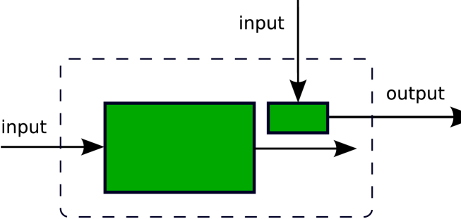
Figure 7: A machine (computer program) that automates the finite element method by automatically generating a particular machine (computer program) for a suitable subset of the given input data.

We also point out that the automation of the finite element method is not only a software engineering problem. In addition to identifying and implementing the proper mathematical concepts, one must develop new mathematical tools and ideas that make it possible for the automating system to realize the full generality of the finite element method. In addition, new insights are needed to build an efficient automating system that can compete with or outperform hand-coded specialized systems for any given input.

8.1 Code Generation

As in all types of engineering, software for scientific computing must try to find a suitable trade-off between generality and efficiency; a software system that is general in nature, that is, it accepts a wide range of inputs, is often less efficient than another software system that performs the same job on a more limited set of inputs. As a result, most codes used by practitioners for the solution of differential equations are very specific, often specialized to a specific method for a specific differential equation.

However, by using a compiler approach, it is possible to combine generality and efficiency without loss of generality and without loss of efficiency. Instead of developing a potentially inefficient general-purpose program that accepts a wide range of inputs, a suitable subset of the input is given to an optimizing compiler that generates a specialized program that takes a more limited set of inputs. In particular, one may automatically generate a specialized simulation code for any given method and differential equation.

An important task is to identify a suitable subset of the input to move to a precompilation phase. In the case of a system automating the solution of differential equations by the finite element method, a suitable subset of input includes the variational problem (29) and the choice of approximating finite element spaces. We thus develop a domain-specific compiler that accepts as input a variational problem and a set of finite elements and generates optimized low-level code (in some general-purpose language such as C or C++). Since the compiler may thus work on only a small family of inputs (multilinear forms), domain-specific knowledge allows the compiler to generate very efficient code, using the optimizations discussed in the previous section. We return to this in more detail below in Section 9.2 when we discuss the FEniCS Form Compiler FFC.

We note that to limit the complexity of the automating system, it is important to identify a minimal set of code to be generated at a precompilation stage, and implement the remaining code in a general-purpose language. It makes less sense to generate the code for administrative tasks such as reading and writing data to file, special algorithms like adaptive mesh refinement etc. These tasks can be implemented as a library in a general-purpose language.

8.2 Just-In-Time Compilation

To make an automating system for the solution of differential equations truly useful, the generation and precompilation of code according to the above discussion must also be automated. Thus, a user should ultimately be presented with a single user-interface and the code should automatically and transparently be generated and compiled just-in-time for a given problem specification.

Achieving just-in-time compilation of variational problems is challenging, not only to construct the exact mechanism by which code is generated, compiled and linked back in at run-time, but also to reduce the precompilation phase to a minimum so that the overhead of code generation and compilation is acceptable. To compile and generate the code for the evaluation of a multilinear form as discussed in Section 5, we need to compute the tensor representation (80), including the evaluation of the reference tensor. Even with an optimized algorithm for the computation of the reference tensor as discussed in [88], the computation of the reference tensor may be very costly, especially for high-order elements and complicated forms. To improve the situation, one may consider caching previously computed reference tensors (similarly to how LaTeX generates and caches fonts in different resolutions) and reuse previously computed reference tensors. As discussed in [88], a reference tensor may be uniquely identified by a (short) string referred to as a signature. Thus, one may store reference tensors along with their signatures to speed up the precomputation and allow run-time just-in-time compilation of variational problems with little overhead.

9 A PROTOTYPE IMPLEMENTATION (FEniCS)

An algorithm must be seen to be believed, and the best way to learn what an algorithm is all about is to try it.

Donald E. Knuth

The Art of Computer Programming (1968)

The automation of the finite element method includes its own realization, that is, a software system that implements the algorithms discussed in Sections 3–6. Such a system is provided by the FEniCS project [60, 36]. We present below some of the key components of FEniCS, including FIAT, FFC and DOLFIN, and point out how they relate to the various aspects of the automation of the finite element method. In particular, the automatic tabulation of finite element basis functions discussed in Section 4 is provided by FIAT [83, 82, 84], the automatic evaluation of the element tensor as discussed in Section 5 is provided by FFC [98, 87, 88, 99] and the automatic assembly of the discrete system as discussed in Section 6 is provided by DOLFIN [62, 68, 63]. The FEniCS project thus serves as a testbed for development of new ideas for the automatic and efficient implementation of finite element methods. At the same, it provides a reference implementation of these ideas.

FEniCS software is free software [55]. In particular, the components of FEniCS are licensed under the GNU General Public License [53]. The source code is freely available on the FEniCS web site [60] and the development is discussed openly on public mailing lists.

9.1 FIAT

The FInite element Automatic Tabulator FIAT [83] was first introduced in [82] and implements the ideas discussed above in Section 4 for the automatic tabulation of finite element basis functions based on a linear algebraic representation of function spaces and constraints.

FIAT provides functionality for defining finite element function spaces as constrained subsets of polynomials on the simplices in one, two and three space dimensions, as well as a library of predefined finite elements, including arbitrary degree Lagrange [27, 20], Hermite [27, 20], Raviart–Thomas [111], Brezzi–Douglas–Marini [22] and Nedelec [106] elements, as well as the (first degree) Crouzeix–Raviart element [31]. Furthermore, the plan is to support Brezzi–Douglas–Fortin–Marini [23] and Arnold–Winther [4] elements in future versions.

In addition to tabulating finite element nodal basis functions (as linear combinations of a reference basis), FIAT generates quadrature points of any given order on the reference simplex and provides functionality for efficient tabulation of the basis functions and their derivatives at any given set of points. In Figure 8 and Figure 9, we present some examples of basis functions generated by FIAT.

Although FIAT is implemented in Python, the interpretive overhead of Python compared to compiled languages is small, since the operations involved may be phrased in terms of standard linear algebra operations, such as the solution of linear systems and singular value decomposition, see [84]. FIAT may thus make use of optimized Python linear algebra libraries such Python Numeric [107]. Recently, a C++ version of FIAT called FIAT++ has also been developed with run-time bindings for Sundance [103, 101, 102].

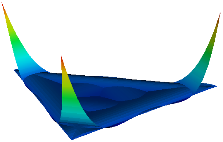
Figure 8: The first three basis functions for a fifth-degree Lagrange finite element on a triangle, associated with the three vertices of the triangle. (Courtesy of Robert C. Kirby.)

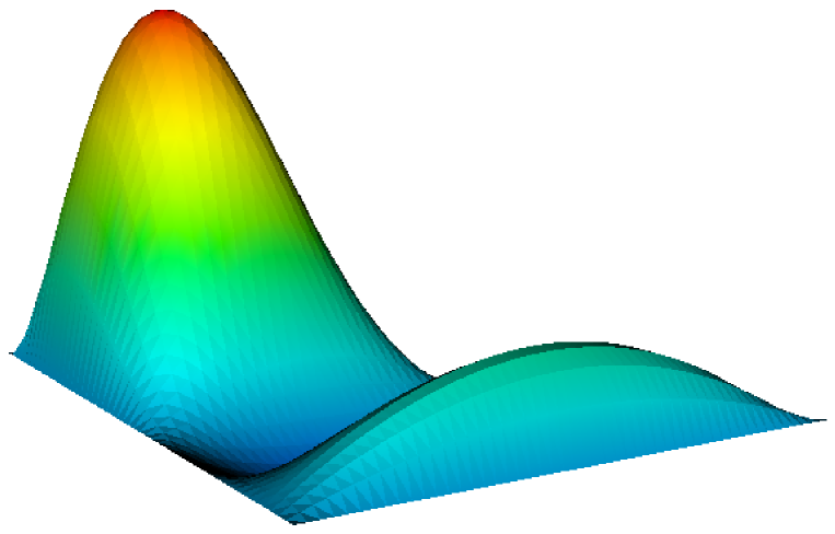
Figure 9: A basis function associated with an interior point for a fifth-degree Lagrange finite element on a triangle. (Courtesy of Robert C. Kirby.)

9.2 FFC

The FEniCS Form Compiler FFC [98], first introduced in [87], automates the evaluation of multilinear forms as outlined in Section 5 by automatically generating code for the efficient computation of the element tensor corresponding to a given multilinear form. FFC thus functions as domain-specific compiler for multilinear forms, taking as input a set of discrete function spaces together with a multilinear form defined on these function spaces, and produces as output optimized low-level code, as illustrated in Figure 10. In its simplest form, FFC generates code in the form of a single C++ header file that can be included in a C++ program, but FFC can also be used as a just-in-time compiler within a scripting environment like Python, for seamless definition and evaluation of multilinear forms.

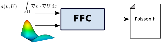
Figure 10: The form compiler FFC takes as input a multilinear form together with a set of function spaces and generates optimized low-level (C++) code for the evaluation of the associated element tensor.

9.2.1 Form language

The FFC form language is generated from a small set of basic data types and operators that allow a user to define a wide range of multilinear forms, in accordance with the discussion of Section 5.4.3. As an illustration, we include below the complete definition in the FFC form language of the bilinear forms for the test cases considered above in Tables 10–13. We refer to the FFC user manual [99] for a detailed discussion of the form language, but note here that in addition to a set of standard operators, including the inner product dot, the partial derivative D, the gradient grad, the divergence div and the rotation rot, FFC supports Einstein tensor-notation (Table 24) and user-defined operators (operator epsilon in Table 25).

 

   

  element = FiniteElement("Lagrange", "tetrahedron", 1) 

  

  v = BasisFunction(element) 

  U = BasisFunction(element) 

  

  a = v*U*dx 

   

 

Table 22: The complete definition of the bilinear form $a(v,U)=\int_{\Omega}v\,U\,\mathrm{d}x$ in the FFC form language (test case 1).

 

   

  element = FiniteElement("Lagrange", "tetrahedron", 1) 

  

  v = BasisFunction(element) 

  U = BasisFunction(element) 

  

  a = dot(grad(v), grad(U))*dx 

   

 

Table 23: The complete definition of the bilinear form $a(v,U)=\int_{\Omega}\nabla v\cdot\nabla U\,\mathrm{d}x$ in the FFC form language (test case 2).

 

   

  element = FiniteElement("Vector Lagrange", "tetrahedron", 1) 

  

  v = BasisFunction(element) 

  U = BasisFunction(element) 

  w = Function(element) 

  

  a = v[i]*w[j]*D(U[i],j)*dx 

   

 

Table 24: The complete definition of the bilinear form $a(v,U)=\int_{\Omega}v\cdot(w\cdot\nabla)U\,\mathrm{d}x$ in the FFC form language (test case 3).

 

   

  element = FiniteElement("Vector Lagrange", "tetrahedron", 1) 

  

  v = BasisFunction(element) 

  U = BasisFunction(element) 

  

  def epsilon(v): 

      return 0.5*(grad(v) + transp(grad(v))) 

  

  a = dot(epsilon(v), epsilon(U))*dx 

   

 

Table 25: The complete definition of the bilinear form $a(v,U)=\int_{\Omega}\epsilon(v):\epsilon(U)\,\mathrm{d}x$ in the FFC form language (test case 4).

9.2.2 Implementation

The FFC form language is implemented in Python as a collection of Python classes (including BasisFunction, Function, FiniteElement etc.) and operators on theses classes. Although FFC is implemented in Python, the interpretive overhead of Python has been minimized by judicious use of optimized numerical libraries such as Python Numeric [107]. The computationally most expensive part of the compilation of a multilinear form is the precomputation of the reference tensor. As demonstrated in [88], by suitably pretabulating basis functions and their derivatives at a set of quadrature points (using FIAT), the reference tensor can be computed by assembling a set of outer products, which may each be efficiently computed by a call to Python Numeric.

Currently, the only optimization FFC makes is to avoid multiplications with any zeros of the reference tensor $A^{0}$ when generating code for the tensor contraction $A^{K}=A^{0}:G_{K}$. As part of the FEniCS project, an optimizing backend, FErari (Finite Element Re-arrangement Algorithm to Reduce Instructions), is currently being developed. Ultimately, FFC will call FErari at compile-time to find an optimized computation of the tensor contraction, according to the discussion in Section 7.

9.2.3 Benchmark results

As a demonstration of the efficiency of the code generated by FFC, we include in Table 26 a comparison taken from [87] between a standard implementation, based on computing the element tensor $A^{K}$ on each cell $K$ by a loop over quadrature points, with the code automatically generated by FFC, based on precomputing the reference tensor $A^{0}$ and computing the element tensor $A^{K}$ by the tensor contraction $A^{K}=A^{0}:G_{K}$ on each cell.

Form	$q=1$	$q=2$	$q=3$	$q=4$	$q=5$	$q=6$	$q=7$	$q=8$
Mass 2D	12	31	50	78	108	147	183	232
Mass 3D	21	81	189	355	616	881	1442	1475
Poisson 2D	8	29	56	86	129	144	189	236
Poisson 3D	9	56	143	259	427	341	285	356
Navier–Stokes 2D	32	33	53	37	—	—	—	—
Navier–Stokes 3D	77	100	61	42	—	—	—	—
Elasticity 2D	10	43	67	97	—	—	—	—
Elasticity 3D	14	87	103	134	—	—	—	—

Table 26: Speedups for test cases 1–4 (Tables 10–13 and Tables 22–25) in two and three space dimensions.

As seen in Table 26, the speedup ranges between one and three orders of magnitude, with larger speedups for higher degree elements. In Figure 11 and Figure 12, we also plot the dependence of the speedup on the polynomial degree for test cases 1 and 2 respectively.

It should be noted that the total work in a simulation also includes the assembly of the local element tensors $\{A^{K}\}_{K\in\mathcal{T}}$ into the global tensor $A$, solving the linear system, iterating on the nonlinear problem etc. Therefore, the overall speedup may be significantly less than the speedups reported in Table 26. We note that if the computation of the local element tensors normally accounts for a fraction $\theta\in(0,1)$ of the total run-time, then the overall speedup gained by a speedup of size $s>1$ for the computation of the element tensors will be

$$1<\frac{1}{1-\theta+\theta/s}\leq\frac{1}{1-\theta},$$ (116)

which is significant only if $\theta$ is significant. As noted in [85], $\theta$ may be significant in many cases, in particular for nonlinear problems where a nonlinear system (or the action of a linear operator) needs to be repeatedly reassembled as part of an iterative method.

\psfrag{q}{$q$}\includegraphics[width=341.43306pt]{eps/ffc-benchmark-mass.eps}

Figure 11: Benchmark results for test case 1, the mass matrix, specified in FFC by a = v*U*dx.

\psfrag{q}{$q$}\includegraphics[width=341.43306pt]{eps/ffc-benchmark-poisson.eps}

Figure 12: Benchmark results for test case 2, Poisson’s equation, specified in FFC by a = dot(grad(v), grad(U))*dx.

9.2.4 User interfaces

FFC can be used either as a stand-alone compiler on the command-line, or as a Python module from within a Python script. In the first case, a multilinear form (or a pair of bilinear and linear forms) is entered in a text file with suffix .form and then compiled by calling the command ffc with the form file on the command-line.

By default, FFC generates C++ code for inclusion in a DOLFIN C++ program (see Section 9.3 below) but FFC can also compile code for other backends (by an appropriate compiler flag), including the ASE (ANL SIDL Environment) format [91], XML format, and LaTeX format (for inclusion of the tensor representation in reports and presentations). The format of the generated code is separated from the parsing of forms and the generation of the tensor contraction, and new formats for alternative backends may be added with little effort, see Figure 13.

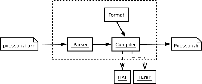
Figure 13: Component diagram for FFC.

Alternatively, FFC can be used directly from within Python as a Python module, allowing definition and compilation of multilinear forms from within a Python script. If used together with the recently developed Python interface of DOLFIN (PyDOLFIN), FFC functions as a just-in-time compiler for multilinear forms, allowing forms to be defined and evaluated from within Python.

9.3 DOLFIN

DOLFIN [62, 68, 63], Dynamic Object-oriented Library for FINite element computation, functions as a general programming interface to DOLFIN and provides a problem-solving environment (PSE) for differential equations in the form of a C++/Python class library.

Initially, DOLFIN was developed as a self-contained (but modularized) C++ code for finite element simulation, providing basic functionality for the definition and automatic evaluation of multilinear forms, assembly, linear algebra, mesh data structures and adaptive mesh refinement, but as a consequence of the development of focused components for each of these tasks as part of the FEniCS project, a large part (but not all) of the functionality of DOLFIN has been delegated to these other components while maintaining a consistent programming interface. Thus, DOLFIN relies on FIAT for the automatic tabulation of finite element basis functions and on FFC for the automatic evaluation of multilinear forms. We discuss below some of the key aspects of DOLFIN and its role as a component of the FEniCS project.

9.3.1 Automatic assembly of the discrete system

DOLFIN implements the automatic assembly of the discrete system associated with a given variational problem as outlined in Section 6. DOLFIN iterates over the cells $\{K\}_{K\in\mathcal{T}}$ of a given mesh $\mathcal{T}$ and calls the code generated by FFC on each cell $K$ to evaluate the element tensor $A^{K}$. FFC also generates the code for the local-to-global mapping which DOLFIN calls to obtain a rule for the addition of each element tensor $A^{K}$ to the global tensor $A$.

Since FFC generates the code for both the evaluation of the element tensor and for the local-to-global mapping, DOLFIN needs to know very little about the finite element method. It only follows the instructions generated by FFC and operates abstractly on the level of Algorithm 2.

9.3.2 Meshes

DOLFIN provides basic data structures and algorithms for simplicial meshes in two and three space dimensions (triangular and tetrahedral meshes) in the form of a class Mesh, including adaptive mesh refinement. As part of PETSc [9, 8, 10] and the FEniCS project, the new component Sieve [81, 80] is currently being developed. Sieve generalizes the mesh concept and provides powerful abstractions for dimension-independent operations on mesh entities and will function as a backend for the mesh data structures in DOLFIN.

9.3.3 Linear algebra

Previously, DOLFIN provided a stand-alone basic linear algebra library in the form of a class Matrix, a class Vector and a collection of iterative and direct solvers. This implementation has recently been replaced by a set of simple wrappers for the sparse linear algebra library provided by PETSc [9, 8, 10]. As a consequence, DOLFIN is able to provide sophisticated high-performance parallel linear algebra with an easy-to-use object-oriented interface suitable for finite element computation.

9.3.4 ODE solvers

DOLFIN also provides a set of general order mono-adaptive and multi-adaptive [94, 95, 50, 97, 100] ODE-solvers, automating the solution of ordinary differential equations. Although the ODE-solvers may be used in connection with the automated assembly of discrete systems, DOLFIN does currently not provide any level of automation for the discretization of time-dependent PDEs. Future versions of DOLFIN (and FFC) will allow time-dependent PDEs to be defined directly in the FFC form language with automatic discretization and adaptive time-integration.

9.3.5 PDE solvers

In addition to providing a class library of basic tools that automate the implementation of adaptive finite element methods, DOLFIN provides a collection of ready-made solvers for a number of standard equations. The current version of DOLFIN provides solvers for Poisson’s equation, the heat equation, the convection–diffusion equation, linear elasticity, updated large-deformation elasticity, the Stokes equations and the incompressible Navier–Stokes equations.

9.3.6 Pre- and post-processing

DOLFIN relies on interaction with external tools for pre-processing (mesh generation) and post-processing (visualization). A number of output formats are provided for visualization, including DOLFIN XML [63], VTK [90] (for use in ParaView [116] or MayaVi [110]), Octave [37], MATLAB [118], OpenDX [1], GiD [28] and Tecplot [2]. DOLFIN may also be easily extended with new output formats.

9.3.7 User interfaces

DOLFIN can be accessed either as a C++ class library or as a Python module, with the Python interface generated semi-automatically from the C++ class library using SWIG [15, 14]. In both cases, the user is presented with a simple and consistent but powerful programming interface.

As discussed in Section 9.3.5, DOLFIN provides a set of ready-made solvers for standard differential equations. In the simplest case, a user thus only needs to supply a mesh, a set of boundary conditions and any parameters and variable coefficients to solve a differential equation, by calling one of the existing solvers. For other differential equations, a solver may be implemented with minimal effort using the set of tools provided by the DOLFIN class library, including variational problems, meshes and linear algebra as discussed above.

9.4 Related Components

We also mention two other projects developed as part of FEniCS. One of these is Puffin[70, 69], a light-weight educational implementation of the basic functionality of FEniCS for Octave/MATLAB, including automatic assembly of the linear system from a given variational problem. Puffin has been used with great success in introductory undergraduate mathematics courses and is accompanied by a set of exercises [79] developed as part of the Body and Soul reform project [48, 41, 42, 40] for applied mathematics education.

The other project is the Ko mechanical simulator [76]. Ko uses DOLFIN as the computational backend and provides a specialized interface to the simulation of mechanical systems, including large-deformation elasticity and collision detection. Ko provides two different modes of simulation: either a simple mass–spring model solved as a system of ODEs, or a large-deformation updated elasticity model [78] solved as a system of time-dependent PDEs. As a consequence of the efficient assembly provided by DOLFIN, based on efficient code being generated by FFC, the overhead of the more complex PDE model compared to the simple ODE model is relatively small.

10 EXAMPLES

In this section, we present a number of examples chosen to illustrate various aspects of the implementation of finite element methods for a number of standard partial differential equations with the FEniCS framework. We already saw in Section 2 the specification of the variational problem for Poisson’s equation in the FFC form language. The examples below include static linear elasticity, two different formulations for the Stokes equations and the time-dependent convection–diffusion equations with the velocity field given by the solution of the Stokes equations. For simplicity, we consider only linear problems but note that the framework allows for implementation of methods for general nonlinear problems. See in particular [78] and [65, 64, 66].

10.1 Static Linear Elasticity

As a first example, consider the equation of static linear elasticity [20] for the displacement $u=u(x)$ of an elastic shape $\Omega\in\mathbb{R}^{d}$,

$$\begin{array}[]{rcll}-\nabla\cdot\sigma(u)&=&f&\mbox{in }\Omega,\\ u&=&u_{0}&\mbox{on }\Gamma_{0}\subset\partial\Omega,\\ \sigma(u)\hat{n}&=&0&\mbox{on }\partial\Omega\setminus\Gamma_{0},\end{array}$$ (117)

where $\hat{n}$ denotes a unit vector normal to the boundary $\partial\Omega$. The stress tensor $\sigma$ is given by

$$\sigma(v)=2\mu\,\epsilon(v)+\lambda\,\mathrm{trace}(\epsilon(v))I,$$ (118)

where $I$ is the $d\times d$ identity matrix and where the strain tensor $\epsilon$ is given by

$$\epsilon(v)=\frac{1}{2}\left(\nabla v+(\nabla v)^{\top}\right),$$ (119)

that is, $\epsilon_{ij}(v)=\frac{1}{2}(\frac{\partial v_{i}}{\partial x_{j}}+\frac{\partial v_{j}}{\partial x_{i}})$ for $i,j=1,\ldots,d$. The Lamé constants $\mu$ and $\lambda$ are given by

$$\mu=\frac{E}{2(1+\nu)},\quad\lambda=\frac{E\nu}{(1+\nu)(1-2\nu)},$$ (120)

with $E$ the Young’s modulus of elasticity and $\nu$ the Poisson ratio, see [121]. In the example below, we take $E=10$ and $\nu=0.3$.

To obtain the discrete variational problem corresponding to (117), we multiply with a test function $v$ in a suitable discrete test space $\hat{V}_{h}$ and integrate by parts to obtain

$$\int_{\Omega}\nabla v:\sigma(U)\,\mathrm{d}x=\int_{\Omega}v\cdot f\,\mathrm{d}x\quad\forall v\in\hat{V}_{h}.$$ (121)

The corresponding formulation in the FFC form language is shown in Table 27 for an approximation with linear Lagrange elements on tetrahedra. Note that by defining the operators $\sigma$ and $\epsilon$, it is possible to obtain a very compact notation that corresponds well with the mathematical notation of (121).

 

   

  element = FiniteElement("Vector Lagrange", "tetrahedron", 1) 

  

  v = BasisFunction(element) 

  U = BasisFunction(element) 

  f = Function(element) 

  

  E  = 10.0 

  nu = 0.3 

  

  mu = E / (2*(1 + nu)) 

  lmbda = E*nu / ((1 + nu)*(1 - 2*nu)) 

  

  def epsilon(v): 

      return 0.5*(grad(v) + transp(grad(v))) 

  

  def sigma(v): 

      return 2*mu*epsilon(v) + lmbda*mult(trace(epsilon(v)), Identity(len(v))) 

  

  a = dot(grad(v), sigma(U))*dx 

  L = dot(v, f)*dx 

   

 

Table 27: The complete specification of the variational problem (121) for static linear elasticity in the FFC form language.

Computing the solution of the variational problem for a domain $\Omega$ given by a gear, we obtain the solution in Figure 14. The gear is clamped at two of its ends and twisted $30$ degrees, as specified by a suitable choice of Dirichlet boundary conditions on $\Gamma_{0}$.

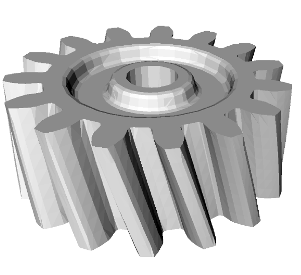
Figure 14: The original domain $\Omega$ of the gear (above) and the twisted gear (below), obtained by displacing $\Omega$ at each point $x\in\Omega$ by the value of the solution $u$ of (117) at the point $x$.

10.2 The Stokes Equations

Next, we consider the Stokes equations,

$$\begin{array}[]{rcll}-\Delta u+\nabla p&=&f&\mbox{in }\Omega,\\ \nabla\cdot u&=&0&\mbox{in }\Omega,\\ u&=&u_{0}&\mbox{on }\partial\Omega,\end{array}$$ (122)

for the velocity field $u=u(x)$ and the pressure $p=p(x)$ in a highly viscous medium. By multiplying the two equations with a pair of test functions $(v,q)$ chosen from a suitable discrete test space $\hat{V}_{h}=\hat{V}_{h}^{u}\times\hat{V}_{h}^{p}$, we obtain the discrete variational problem

$$\int_{\Omega}\nabla v:\nabla U-(\nabla\cdot v)P+q\nabla\cdot U\,\mathrm{d}x=\int_{\Omega}v\cdot f\,\mathrm{d}x\quad\forall(v,q)\in\hat{V}_{h}.$$ (123)

for the discrete approximate solution $(U,P)\in V_{h}=V^{u}_{h}\times V^{p}_{h}$. To guarantee the existence of a unique solution of the discrete variational problem (123), the discrete function spaces $\hat{V}_{h}$ and $V_{h}$ must be chosen appropriately. The Babuška–Brezzi [5, 21] inf–sup condition gives a precise condition for the selection of the approximating spaces.

10.2.1 Taylor–Hood elements

One way to fulfill the Babuška–Brezzi condition is to use different order approximations for the velocity and the pressure, such as degree $q$ polynomials for the velocity and degree $q-1$ for the pressure, commonly referred to as Taylor–Hood elements, see [19, 20]. The resulting mixed formulation may be specified in the FFC form language by defining a Taylor–Hood element as the direct sum of a degree $q$ vector-valued Lagrange element and a degree $q-1$ scalar Lagrange element, as shown in Table 28. Figure 16 shows the velocity field for the flow around a two-dimensional dolphin computed with a $P_{2}$–$P_{1}$ Taylor-Hood approximation.

 

   

  P2 = FiniteElement("Vector Lagrange", "triangle", 2) 

  P1 = FiniteElement("Lagrange", "triangle", 1) 

  TH = P2 + P1 

  

  (v, q) = BasisFunctions(TH) 

  (U, P) = BasisFunctions(TH) 

  

  f = Function(P2) 

  

  a = (dot(grad(v), grad(U)) - div(v)*P + q*div(U))*dx 

  L = dot(v, f)*dx 

   

 

Table 28: The complete specification of the variational problem (123) for the Stokes equations with $P_{2}$–$P_{1}$ Taylor–Hood elements.

10.2.2 A stabilized equal-order formulation

Alternatively, the Babuška–Brezzi condition may be circumvented by an appropriate modification (stabilization) of the variational problem (123). In general, an appropriate modification may be obtained by a Galerkin/least-squares (GLS) stabilization, that is, by modifying the test function $w=(v,q)$ according to $w\rightarrow w+\delta Aw$, where $A$ is the operator of the differential equation and $\delta=\delta(x)$ is suitable stabilization parameter. Here, we a choose simple pressure-stabilization obtained by modifying the test function $w=(v,q)$ according to

$$(v,q)\rightarrow(v,q)+(\delta\nabla q,0).$$ (124)

The stabilization (124) is sometimes referred to as a pressure-stabilizing/Petrov-Galerkin (PSPG) method, see [72, 56]. Note that the stabilization (124) may also be viewed as a reduced GLS stabilization.

We thus obtain the following modified variational problem: Find $(U,P)\in V_{h}$ such that

$$\int_{\Omega}\nabla v:\nabla U-(\nabla\cdot v)P+q\nabla\cdot U+\delta\nabla q\cdot\nabla P\,\mathrm{d}x=\int_{\Omega}(v+\delta\nabla q)\cdot f\,\mathrm{d}x\quad\forall(v,q)\in\hat{V}_{h}.$$ (125)

Table 29 shows the stabilized equal-order method in the FFC form language, with the stabilization parameter given by

$$\delta=\beta h^{2},$$ (126)

where $\beta=0.2$ and $h=h(x)$ is the local mesh size (cell diameter).

 

   

  vector = FiniteElement("Vector Lagrange", "triangle", 1) 

  scalar = FiniteElement("Lagrange", "triangle", 1) 

  system = vector + scalar 

  

  (v, q) = BasisFunctions(system) 

  (U, P) = BasisFunctions(system) 

  

  f = Function(vector) 

  h = Function(scalar) 

  

  d = 0.2*h*h 

  

  a = (dot(grad(v), grad(U)) - div(v)*P + q*div(U) + d*dot(grad(q), grad(P)))*dx 

  L = dot(v + mult(d, grad(q)), f)*dx 

   

 

Table 29: The complete specification of the variational problem (125) for the Stokes equations with an equal-order $P_{1}$–$P_{1}$ stabilized method.

In Figure 15, we illustrate the importance of stabilizing the equal-order method by plotting the solution for the pressure with and without stabilization. Without stabilization, the solution oscillates heavily. Note that the scaling is chosen differently in the two images, with the oscillations scaled down by a factor two in the unstabilized solution. The situation without stabilization is thus even worse than what the figure indicates.

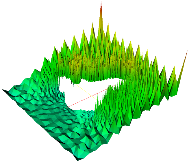
Figure 15: The pressure for the flow around a two-dimensional dolphin, obtained by solving the Stokes equations (122) by an unstabilized $P_{1}$–$P_{1}$ approximation (above) and a stabilized $P_{1}$–$P_{1}$ approximation (below).

10.3 Convection–Diffusion

As a final example, we compute the temperature $u=u(x,t)$ around the dolphin (Figure 17) from the previous example by solving the time-dependent convection–diffusion equations,

$$\begin{array}[]{rcll}\dot{u}+b\cdot\nabla u-\nabla\cdot(c\nabla u)&=&f&\mbox{in }\Omega\times(0,T],\\ u&=&u_{\partial}&\mbox{on }\partial\Omega\times(0,T],\\ u&=&u_{0}&\mbox{at }\Omega\times\{0\},\end{array}$$ (127)

with velocity field $b=b(x)$ obtained by solving the Stokes equations.

Figure 16: The velocity field for the flow around a two-dimensional dolphin, obtained by solving the Stokes equations (122) by a $P_{2}$–$P_{1}$ Taylor-Hood approximation.

Figure 17: The temperature around a hot dolphin in surrounding cold water with a hot inflow, obtained by solving the convection–diffusion equation with the velocity field obtained from a solution of the Stokes equations with a $P_{2}$–$P_{1}$ Taylor–Hood approximation.

We discretize (127) with the $\mathrm{cG}(1)\mathrm{cG}(1)$ method, that is, with continuous piecewise linear functions in space and time (omitting stabilization for simplicity). The interval $[0,T]$ is partitioned into a set of time intervals $0=t_{0}<t_{1}<\cdots<t_{n-1}<t_{n}<\cdots<t_{M}=T$ and on each time interval $(t_{n-1},t_{n}]$, we pose the variational problem

$$\int_{t_{n-1}}^{t_{n}}\int_{\Omega}(v,\dot{U})+v\,b\cdot\nabla U+c\nabla v\cdot\nabla U\,\mathrm{d}x\,\mathrm{d}t=\int_{t_{n-1}}^{t_{n}}\int_{\Omega}v\,f\,\mathrm{d}x\,\mathrm{d}t\quad\forall v\in\hat{V}_{h},$$ (128)

with $\hat{V}_{h}$ the space of all continuous piecewise linear functions in space. Note that the $\mathrm{cG}(1)$ method in time uses piecewise constant test functions, see [74, 73, 51, 39, 94]. As a consequence, we obtain the following variational problem for $U^{n}\in V_{h}=\hat{V}_{h}$, the piecewise linear in space solution at time $t=t_{n}$,

$$\begin{split}\int_{\Omega}v\,\frac{U^{n}-U^{n-1}}{k_{n}}+v\,b\cdot\nabla(U^{n}+U^{n-1})/2+c\,\nabla v\cdot\nabla(U^{n}+U^{n-1})/2\,\mathrm{d}x\\ =\int_{t_{n-1}}^{t_{n}}\int_{\Omega}v\,f\,\mathrm{d}x\,\mathrm{d}t\quad\forall v\in\hat{V}_{h},\end{split}$$ (129)

where $k_{n}=t_{n}-t_{n-1}$ is the size of the time step. We thus obtain a variational problem of the form

$$a(v,U^{n})=L(v)\quad\forall v\in\hat{V}_{h},$$ (130)

where

$$\begin{split}a(v,U^{n})&=\int_{\Omega}v\,U^{n}\,\mathrm{d}x+\frac{k_{n}}{2}\left(v\,b\cdot\nabla U^{n}+c\,\nabla v\cdot\nabla U^{n}\right)\,\mathrm{d}x,\\ L(v)&=\int_{\Omega}v\,U^{n-1}\,\mathrm{d}x-\frac{k_{n}}{2}\left(v\,b\cdot\nabla U^{n-1}+c\,\nabla v\cdot\nabla U^{n-1}\right)\,\mathrm{d}x+\int_{t_{n-1}}^{t_{n}}\int_{\Omega}v\,f\,\mathrm{d}x\,\mathrm{d}t.\end{split}$$ (131)

The corresponding specification in the FFC form language is presented in Table 30, where for simplicity we approximate the right-hand side with its value at the right end-point.

 

   

 scalar = FiniteElement("Lagrange", "triangle", 1) 

 vector = FiniteElement("Vector Lagrange", "triangle", 2) 

  

 v  = BasisFunction(scalar) 

 U1 = BasisFunction(scalar) 

 U0 = Function(scalar) 

 b  = Function(vector) 

 f  = Function(scalar) 

  

 c = 0.005 

 k = 0.05 

  

 a = v*U1*dx + 0.5*k*(v*dot(b, grad(U1)) + c*dot(grad(v), grad(U1)))*dx 

 L = v*U0*dx - 0.5*k*(v*dot(b, grad(U0)) + c*dot(grad(v), grad(U0)))*dx + k*v*f*dx 

   

 

Table 30: The complete specification of the variational problem (130) for $\mathrm{cG}(1)$ time-stepping of the convection–diffusion equation.

11 OUTLOOK: THE AUTOMATION OF CMM

The automation of the finite element method, as described above, constitutes an important step towards the Automation of Computational Mathematical Modeling (ACMM), as outlined in [96]. In this context, the automation of the finite element method amounts to the automation of discretization, that is, the automatic translation of a given continuous model to a system of discrete equations. Other key steps include the automation of discrete solution, the automation of error control, the automation of modeling and the automation of optimization. We discuss these steps below and also make some comments concerning automation in general.

11.1 The Principles of Automation

An automatic system carries out a well-defined task without intervention from the person or system actuating the automatic process. The task of the automating system may be formulated as follows: For given input satisfying a fixed set of conditions (the input conditions), produce output satisfying a given set of conditions (the output conditions).

An automatic process is defined by an algorithm, consisting of a sequential list of instructions (like a computer program). In automated manufacturing, each step of the algorithm operates on and transforms physical material. Correspondingly, an algorithm for the Automation of CMM operates on digits and consists of the automated transformation of digital information.

A key problem of automation is the design of a feed-back control, allowing the given output conditions to be satisfied under variable input and external conditions, ideally at a minimal cost. Feed-back control is realized through measurement, evaluation and action; a quantity relating to the given set of conditions to be satisfied by the output is measured, the measured quantity is evaluated to determine if the output conditions are satisfied or if an adjustment is necessary, in which case some action is taken to make the necessary adjustments. In the context of an algorithm for feed-back control, we refer to the evaluation of the set of output conditions as the stopping criterion, and to the action as the modification strategy.

A key step in the automation of a complex process is modularization, that is, the hierarchical organization of the complex process into components or sub processes. Each sub process may then itself be automated, including feed-back control. We may also express this as abstraction, that is, the distinction between the properties of a component (its purpose) and the internal workings of the component (its realization).

Modularization (or abstraction) is central in all engineering and makes it possible to build complex systems by connecting together components or subsystems without concern for the internal workings of each subsystem. The exact partition of a system into components is not unique. Thus, there are many ways to partition a system into components. In particular, there are many ways to design a system for the Automation of Computational Mathematical Modeling.

We thus identify the following basic principles of automation: algorithms, feed-back control, and modularization.

11.2 Computational Mathematical Modeling

In automated manufacturing, the task of the automating system is to produce a certain product (the output) from a given piece of material (the input), with the product satisfying some measure of quality (the output conditions).

\psfrag{in1}{$A(u)=f$}\psfrag{in2}{$\mathrm{TOL}>0$}\psfrag{ut}{\hskip 11.38092pt $U\approx u$}\includegraphics[width=341.43306pt]{eps/automation-2-1.eps}

Figure 18: The Automation of Computational Mathematical Modeling.

For the Automation of CMM, the input is a given model of the form

$$A(u)=f,$$ (132)

for the solution $u$ on a given domain $\Omega\times(0,T]$ in space-time, where $A$ is a given differential operator and where $f$ is a given source term. The output is a discrete solution $U\approx u$ satisfying some measure of quality. Typically, the measure of quality is given in the form of a tolerance $\mathrm{TOL}>0$ for the size of the error $e=U-u$ in a suitable norm, $\|e\|\leq\mathrm{TOL}$, or alternatively, the error in some given functional $M$,

$$\left|M(U)-M(u)\right|\leq\mathrm{TOL}.$$ (133)

In addition to controlling the quality of the computed solution, one may also want to determine a parameter that optimizes some given cost functional depending on the computed solution (optimization). We refer to the overall process, including optimization, as the Automation of CMM.

The key problem for the Automation of CMM is thus the design of a feed-back control for the automatic construction of a discrete solution $U$, satisfying the output condition (133) at minimal cost. The design of this feed-back control is based on the solution of an associated dual problem, connecting the size of the residual $R(U)=A(U)-f$ of the computed discrete solution to the size of the error $e$, and thus to the output condition (133).

11.3 An Agenda for the Automation of CMM

Following our previous discussion on modularization as a basic principle of automation, we identify the following key steps in the Automation of CMM:

• the automation of discretization, that is, the automatic translation of a continuous model of the form (132) to a system of discrete equations;

• the automation of discrete solution, that is, the automatic solution of the system of discrete equations obtained from the automatic discretization of (132),

• the automation of error control, that is, the automatic selection of an appropriate resolution of the discrete model to produce a discrete solution satisfying the given accuracy requirement with minimal work;

• the automation of modeling, that is, the automatic selection of the model (132), either by constructing a model from a given set of data, or by constructing from a given model a reduced model for the variation of the solution on resolvable scales;

• the automation of optimization, that is, the automatic selection of a parameter in the model (132) to optimize a given goal functional.

In Figure 19, we demonstrate how (i)–(iv) connect to solve the overall task of the Automation of CMM (excluding optimization) in accordance with Figure 18. We discuss (i)–(v) in some detail below. In all cases, feed-back control, or adaptivity, plays a key role.

\psfrag{eq}{$A(u)=f$}\psfrag{TOL}{$\mathrm{TOL}$}\psfrag{U}{$U\approx u$}\psfrag{tol}{$\mathrm{tol}>0$}\psfrag{eq2}{$A(\bar{u})=\bar{f}+\bar{g}(u)$}\psfrag{V}{$(\hat{V}_{h},V_{h})$}\psfrag{F}{$F(x)=0$}\psfrag{X}{$X\approx x$}\includegraphics[width=398.33858pt]{eps/automation-of-computation.eps}

Figure 19: A modularized view of the Automation of Computational Mathematical Modeling.

11.4 The Automation of Discretization

The automation of discretization amounts to automatically generating a system of discrete equations for the degrees of freedom of a discrete solution $U$ approximating the solution $u$ of the given model (132), or alternatively, the solution $u\in V$ of a corresponding variational problem

$$a(u;v)=L(v)\quad\forall v\in\hat{V},$$ (134)

where as before $a:V\times\hat{V}\rightarrow\mathbb{R}$ is a semilinear form which is linear in its second argument and $L:\hat{V}\rightarrow\mathbb{R}$ is a linear form. As we saw in Section 3, this process may be automated by the finite element method, by replacing the function spaces $(\hat{V},V)$ with a suitable pair $(\hat{V}_{h},V_{h})$ of discrete function spaces, and an approach to its automation was discussed in Sections 4–6. As we shall discuss further below, the pair of discrete function spaces may be automatically chosen by feed-back control to compute the discrete solution $U$ both reliably and efficiently.

11.5 The Automation of Discrete Solution

Depending on the model (132) and the method used to automatically discretize the model, the resulting system of discrete equations may require more or less work to solve. Typically, the discrete system is solved by some iterative method such as the conjugate gradient method (CG) or GMRES, in combination with an appropriate choice of preconditioner, see for example [114, 32].

The resolution of the discretization of (132) may be chosen automatically by feed-back control from the computed solution, with the target of minimizing the computational work while satisfying a given accuracy requirement. As a consequence, see for example [94], one obtains an accuracy requirement on the solution of the system of discrete equations. Thus, the system of discrete equations does not need to be solved to within machine precision, but only to within some discrete tolerance $\mathrm{tol>0}$ for some error in a functional of the solution of the discrete system. We shall not pursue this question further here, but remark that the feed-back control from the computed solution to the iterative algorithm for the solution of the system of discrete equations is often weak, and the problem of designing efficient adaptive iterative algorithms for the system of discrete equations remains open.

11.6 The Automation of Error Control

As stated above, the overall task is to produce a solution of (132) that satisfies a given accuracy requirement with minimal work. This includes an aspect of reliability, that is, the error in an output quantity of interest depending on the computed solution should be less than a given tolerance, and an aspect of efficiency, that is, the solution should be computed with minimal work. Ideally, an algorithm for the solution of (132) should thus have the following properties: Given a tolerance $\mathrm{TOL}>0$ and a functional $M$, the algorithm shall produce a discrete solution $U$ approximating the exact solution $u$ of (132), such that

• $|M(U)-M(u)|\leq\mathrm{TOL}$;

• the computational cost of obtaining the approximation $U$ is minimal.

Conditions (A) and (B) can be satisfied by an adaptive algorithm, with the construction of the discrete representation $(\hat{V}_{h},V_{h})$ based on feed-back from the computed solution.

An adaptive algorithm typically involves a stopping criterion, indicating that the size of the error is less than the given tolerance, and a modification strategy to be applied if the stopping criterion is not satisfied. Often, the stopping criterion and the modification strategy are based on an a posteriori error estimate $E\geq|M(U)-M(u)|$, estimating the error in terms of the residual $R(U)=A(U)-f$ and the solution $\varphi$ of a dual problem connecting to the stability of (132).

11.6.1 The dual problem

The dual problem of (132) for the given output functional $M$ is given by

$$\overline{A^{\prime}}^{*}\varphi=\psi,$$ (135)

on $\Omega\times[0,T)$, where $\overline{A^{\prime}}^{*}$ denotes the adjoint of the Fréchet derivative $A^{\prime}$ of $A$ evaluated at a suitable mean value of the exact solution $u$ and the computed solution $U$,

$$\overline{A^{\prime}}=\int_{0}^{1}A^{\prime}\left(sU+(1-s)u\right)\,\mathrm{d}s,$$ (136)

and where $\psi$ is the Riesz representer of a similar mean value of the Fréchet derivative $M^{\prime}$ of $M$,

$$(v,\psi)=\overline{M^{\prime}}v\quad\forall v\in V.$$ (137)

By the dual problem (135), we directly obtain the error representation

$$\begin{split}M(U)-M(u)&=\overline{M^{\prime}}(U-u)=(U-u,\psi)=(U-u,\overline{A^{\prime}}^{*}\varphi)=(\overline{A^{\prime}}(U-u),\varphi)\\ &=(A(U)-A(u),\varphi)=(A(U)-f,\varphi)=(R(U),\varphi).\end{split}$$ (138)

Noting now that if the solution $U$ is computed by a Galerkin method and thus $(R(U),v)=0$ for any $v\in\hat{V}_{h}$, we obtain

$$M(U)-M(u)=(R(U),\varphi-\pi_{h}\varphi),$$ (139)

where $\pi_{h}\varphi$ is a suitable approximation of $\varphi$ in $\hat{V}_{h}$. One may now proceed to estimate the error $M(U)-M(u)$ in various ways, either by estimating the interpolation error $\pi_{h}\varphi-\varphi$ or by directly evaluating the quantity $(R(U),\varphi-\pi_{h}\varphi)$. The residual $R(U)$ and the dual solution $\varphi$ give precise information about the influence of the discrete representation $(\hat{V}_{h},V_{h})$ on the size of the error, which can be used in an adaptive feed-back control to choose a suitable discrete representation for the given output quantity $M$ of interest and the given tolerance $\mathrm{TOL}$ for the error, see [38, 17, 52, 94].

11.6.2 The weak dual problem

We may estimate the error similarly for the variational problem (134) by considering the following weak (variational) dual problem: Find $\varphi\in\hat{V}$ such that

$$\overline{a^{\prime}}^{*}(U,u;\,v,\varphi)=\overline{M^{\prime}}(U,u;v)\quad\forall v\in V,$$ (140)

where $\overline{a^{\prime}}^{*}$ denotes the adjoint of the bilinear form $\overline{a^{\prime}}$, given as above by an appropriate mean value of the Fréchet derivative of the semilinear form $a$. We now obtain the error representation

$$\begin{split}M(U)-M(u)&=\overline{M^{\prime}}(U,u;\,U-u)=\overline{a^{\prime}}^{*}(U,u;\,U-u,\varphi)=\overline{a^{\prime}}(U,u;\,\varphi,U-u)\\ &=a(U;\,\varphi)-a(u;\,\varphi)=a(U;\,\varphi)-L(\varphi).\end{split}$$ (141)

As before, we use the Galerkin orthogonality to subtract $a(U;\pi\varphi)-L(\pi\varphi)=0$ for some $\pi_{h}\varphi\in\hat{V}_{h}\subset\hat{V}$ and obtain

$$M(U)-M(u)=a(U;\varphi-\pi\varphi)-L(\varphi-\pi\varphi).$$ (142)

To automate the process of error control, we thus need to automatically generate and solve the dual problem (135) or (140) from a given primal problem (132) or (134). We investigate this question further in [61].

11.7 The Automation of Modeling

The automation of modeling concerns both the problem of finding the parameters describing the model (132) from a given set of data (inverse modeling), and the automatic construction of a reduced model for the variation of the solution on resolvable scales (model reduction). We here discuss briefly the automation of model reduction.

In situations where the solution $u$ of (132) varies on scales of different magnitudes, and these scales are not localized in space and time, computation of the solution may be very expensive, even with an adaptive method. To make computation feasible, one may instead seek to compute an average $\bar{u}$ of the solution $u$ of (132) on resolvable scales. Typical examples include meteorological models for weather prediction, with fast time scales on the range of seconds and slow time scales on the range of years, or protein folding represented by a molecular dynamics model, with fast time scales on the range of femtoseconds and slow time scales on the range of microseconds.

Model reduction typically involves extrapolation from resolvable scales, or the construction of a large-scale model from local resolution of fine scales in time and space. In both cases, a large-scale model

$$A(\bar{u})=\bar{f}+\bar{g}(u),$$ (143)

for the average $\bar{u}$ is constructed from the given model (132) with a suitable modeling term $\bar{g}(u)\approx A(\bar{u})-\bar{A}(u)$.

Replacing a given model with a computable reduced model by taking averages in space and time is sometimes referred to as subgrid modeling. Subgrid modeling has received much attention in recent years, in particular for the incompressible Navier–Stokes equations, where the subgrid modeling problem takes the form of determining the Reynolds stresses corresponding to $\bar{g}$. Many subgrid models have been proposed for the averaged Navier–Stokes equations, but no clear answer has been given. Alternatively, the subgrid model may take the form of a least-squares stabilization, as suggested in [65, 64, 66]. In either case, the validity of a proposed subgrid model may be verified computationally by solving an appropriate dual problem and computing the relevant residuals to obtain an error estimate for the modeling error, see [77].

11.8 The Automation of Optimization

The automation of optimization relies on the automation of (i)–(iv), with the solution of the primal problem (132) and an associated dual problem being the key steps in the minimization of a given cost functional. In particular, the automation of optimization relies on the automatic generation of the dual problem.

The optimization of a given cost functional $\mathcal{J}=\mathcal{J}(u,p)$, subject to the constraint (132), with $p$ a function (the control variables) to be determined, can be formulated as the problem of finding a stationary point of the associated Lagrangian,

$$L(u,p,\varphi)=\mathcal{J}(u,p)+(A(u,p)-f(p),\varphi),$$ (144)

which takes the form of a system of differential equations, involving the primal and dual problems, as well as an equation expressing stationarity with respect to the control variables $p$,

$$\begin{split}A(u,p)&=f(p),\\ (A^{\prime})^{*}(u,p)\varphi&=-\partial\mathcal{J}/\partial u,\\ \partial\mathcal{J}/\partial p&=(\partial f/\partial p)^{*}\varphi-(\partial A/\partial p)^{*}\varphi.\\ \end{split}$$ (145)

It follows that the optimization problem may be solved by the solution of a system of differential equations. Note that the first equation is the given model (132), the second equation is the dual problem and the third equation gives a direction for the update of the control variables. The automation of optimization thus relies on the automated solution of both the primal problem (132) and the dual problem (135), including the automatic generation of the dual problem.

12 CONCLUDING REMARKS

With the FEniCS project [60], we have the beginnings of a working system automating (in part) the finite element method, which is the first step towards the Automation of Computational Mathematical Modeling, as outlined in [96]. As part of this work, a number of key components, FIAT, FFC and DOLFIN, have been developed. These components provide reference implementations of the algorithms discussed in Sections 3–6.

As the current toolset, focused mainly on an automation of the finite element method (the automation of discretization), is becoming more mature, important new areas of research and development emerge, including the remaining key steps towards the Automation of CMM. In particular, we plan to explore the possibility of automatically generating dual problems and error estimates in an effort to automate error control.

NOTATION

$A$	–	the differential operator of the model $A(u)=f$
$A$	–	the global tensor with entries $\{A_{i}\}_{i\in\mathcal{I}}$
$A^{0}$	–	the reference tensor with entries $\{A^{0}_{i\alpha}\}_{i\in\mathcal{I}_{K},\alpha\in\mathcal{A}}$
$\bar{A}^{0}$	–	the matrix representation of the (flattened) reference tensor $A^{0}$
$A^{K}$	–	the element tensor with entries $\{A^{K}_{i}\}_{i\in\mathcal{I}_{K}}$
$a$	–	the semilinear, multilinear or bilinear form
$a_{K}$	–	the local contribution to a multilinear form $a$ from $K$
$a^{K}$	–	the vector representation of the (flattened) element tensor $A^{K}$
$\mathcal{A}$	–	the set of secondary indices
$\mathcal{B}$	–	the set of auxiliary indices
$e$	–	the error, $e=U-u$
$F_{K}$	–	the mapping from $K_{0}$ to $K$
$G_{K}$	–	the geometry tensor with entries $\{G_{K}^{\alpha}\}_{\alpha\in\mathcal{A}}$
$g_{K}$	–	the vector representation of the (flattened) geometry tensor $G_{K}$
$\mathcal{I}$	–	the set $\prod_{j=1}^{r}[1,N^{j}]$ of indices for the global tensor $A$
$\mathcal{I}_{K}$	–	the set $\prod_{j=1}^{r}[1,n_{K}^{j}]$ of indices for the element tensor $A^{K}$ (primary indices)
$\iota_{K}$	–	the local-to-global mapping from $\mathcal{N}_{K}$ to $\mathcal{N}$
$\hat{\iota}_{K}$	–	the local-to-global mapping from $\hat{\mathcal{N}}_{K}$ to $\hat{\mathcal{N}}$
$\iota_{K}^{j}$	–	the local-to-global mapping from $\mathcal{N}_{K}^{j}$ to $\mathcal{N}^{j}$
$K$	–	a cell in the mesh $\mathcal{T}$
$K_{0}$	–	the reference cell
$L$	–	the linear form (functional) on $\hat{V}$ or $\hat{V}_{h}$
$m$	–	the number of discrete function spaces used in the definition of $a$
$N$	–	the dimension of $\hat{V}_{h}$ and $V_{h}$
$N^{j}$	–	the dimension $V_{h}^{j}$
$N_{q}$	–	the number of quadrature points on a cell
$n_{0}$	–	the dimension of $\mathcal{P}_{0}$
$n_{K}$	–	the dimension of $\mathcal{P}_{K}$
$\hat{n}_{K}$	–	the dimension of $\hat{\mathcal{P}}_{K}$
$n_{K}^{j}$	–	the dimension of $\mathcal{P}_{K}^{j}$
$\mathcal{N}$	–	the set of global nodes on $V_{h}$
$\hat{\mathcal{N}}$	–	the set of global nodes on $\hat{V}_{h}$
$\mathcal{N}^{j}$	–	the set of global nodes on $V_{h}^{j}$
$\mathcal{N}_{0}$	–	the set of local nodes on $\mathcal{P}_{0}$
$\mathcal{N}_{K}$	–	the set of local nodes on $\mathcal{P}_{K}$
$\hat{\mathcal{N}}_{K}$	–	the set of local nodes on $\hat{\mathcal{P}}_{K}$
$\mathcal{N}_{K}^{j}$	–	the set of local nodes on ${\mathcal{P}_{K}^{j}}$

$\nu^{0}_{i}$	–	a node on $\mathcal{P}_{0}$
$\nu^{K}_{i}$	–	a node on $\mathcal{P}_{K}$
$\hat{\nu}^{K}_{i}$	–	a node on $\hat{\mathcal{P}}_{K}$
$\nu^{K,j}_{i}$	–	a node on $\mathcal{P}_{K}^{j}$
$\mathcal{P}_{0}$	–	the function space on $K_{0}$ for $V_{h}$
$\hat{\mathcal{P}}_{0}$	–	the function space on $K_{0}$ for $\hat{V}_{h}$
$\mathcal{P}_{0}^{j}$	–	the function space on $K_{0}$ for $V_{h}^{j}$
$\mathcal{P}_{K}$	–	the local function space on $K$ for $V_{h}$
$\hat{\mathcal{P}}_{K}$	–	the local function space on $K$ for $\hat{V}_{h}$
$\mathcal{P}_{K}^{j}$	–	the local function space on $K$ for $V_{h}^{j}$
$P_{q}(K)$	–	the space of polynomials of degree $\leq q$ on $K$
$\overline{\mathcal{P}}_{K}$	–	the local function space on $K$ generated by $\{\mathcal{P}_{K}^{j}\}_{j=1}^{m}$
$R$	–	the residual, $R(U)=A(U)-f$
$r$	–	the arity of the multilinear form $a$ (the rank of $A$ and $A^{K}$)
$U$	–	the discrete approximate solution, $U\approx u$
$(U_{i})$	–	the vector of expansion coefficients for $U=\sum_{i=1}^{N}U_{i}\phi_{i}$
$u$	–	the exact solution of the given model $A(u)=f$
$V$	–	the space of trial functions on $\Omega$ (the trial space)
$\hat{V}$	–	the space of test functions on $\Omega$ (the test space)
$V_{h}$	–	the space of discrete trial functions on $\Omega$ (the discrete trial space)
$\hat{V}_{h}$	–	the space of discrete test functions on $\Omega$ (the discrete test space)
$V_{h}^{j}$	–	a discrete function space on $\Omega$
$|V|$	–	the dimension of a vector space $V$
$\Phi_{i}$	–	a basis function in $\mathcal{P}_{0}$
$\hat{\Phi}_{i}$	–	a basis function in $\hat{\mathcal{P}}_{0}$
$\Phi_{i}^{j}$	–	a basis function in $\mathcal{P}_{0}^{j}$
$\phi_{i}$	–	a basis function in $V_{h}$
$\hat{\phi}_{i}$	–	a basis function in $\hat{V}_{h}$
$\phi_{i}^{j}$	–	a basis function in $V_{h}^{j}$
$\phi_{i}^{K}$	–	a basis function in $\mathcal{P}_{K}$
$\hat{\phi}_{i}^{K}$	–	a basis function in $\hat{\mathcal{P}}_{K}$
$\phi_{i}^{K,j}$	–	a basis function in $\mathcal{P}_{K}^{j}$
$\varphi$	–	the dual solution
$\mathcal{T}$	–	the mesh
$\Omega$	–	a bounded domain in $\mathbb{R}^{d}$

References

- [1] OpenDX, 2006. URL: http://www.opendx.org/.
- [2] Tecplot, 2006. URL: http://www.tecplot.com/.
- [3] S. E. Arge, A. M. Bruaset, and H. P. Langtangen, eds., Modern Software Tools for Scientific Computing, Birkhäuser, 1997.
- [4] D. N. Arnold and R. Winther, Mixed finite elements for elasticity, Numer. Math., 92 (2002), pp. 401–419.
- [5] I. Babuška, Error bounds for finite element method, Numer. Math., 16 (1971), pp. 322–333.
- [6] B. Bagheri and L. R. Scott, Analysa, 2003. URL: http://people.cs.uchicago.edu/~ridg/al/aa.html.
- [7] B. Bagheri and L. R. Scott, About Analysa, Tech. Rep. TR–2004–09, University of Chicago, Department of Computer Science, 2004.
- [8] S. Balay, K. Buschelman, V. Eijkhout, W. D. Gropp, D. Kaushik, M. G. Knepley, L. C. McInnes, B. F. Smith, and H. Zhang, PETSc users manual, Tech. Rep. ANL-95/11 - Revision 2.1.5, Argonne National Laboratory, 2004.
- [9] S. Balay, K. Buschelman, W. D. Gropp, D. Kaushik, M. G. Knepley, L. C. McInnes, B. F. Smith, and H. Zhang, PETSc, 2006. URL: http://www.mcs.anl.gov/petsc/.
- [10] S. Balay, V. Eijkhout, W. D. Gropp, L. C. McInnes, and B. F. Smith, Efficient management of parallelism in object oriented numerical software libraries, in Modern Software Tools in Scientific Computing, E. Arge, A. M. Bruaset, and H. P. Langtangen, eds., Birkhäuser Press, 1997, pp. 163–202.
- [11] W. Bangerth, Using modern features of C++ for adaptive finite element methods: Dimension-independent programming in deal.II, in Proceedings of the 16th IMACS World Congress 2000, Lausanne, Switzerland, 2000, M. Deville and R. Owens, eds., 2000. Document Sessions/118-1.
- [12] W. Bangerth, R. Hartmann, and G. Kanschat, deal.II Differential Equations Analysis Library, 2006. URL: http://www.dealii.org/.
- [13] W. Bangerth and G. Kanschat, Concepts for object-oriented finite element software – the deal.II library, Preprint 99-43 (SFB 359), IWR Heidelberg, Oct. 1999.
- [14] D. M. Beazley, SWIG : An easy to use tool for integrating scripting languages with C and C++, presented at the 4th Annual Tcl/Tk Workshop, Monterey, CA, (2006).
- [15] D. M. Beazley et al., Simplified Wrapper and Interface Generator, 2006. URL: http://www.swig.org/.
- [16] E. B. Becker, G. F. Carey, and J. T. Oden, Finite Elements: An Introduction, Prentice–Hall, Englewood–Cliffs, 1981.
- [17] R. Becker and R. Rannacher, An optimal control approach to a posteriori error estimation in finite element methods, Acta Numerica, 10 (2001), pp. 1–102.
- [18] L. S. Blackford, J. Demmel, J. Dongarra, I. Duff, S. Hammarling, G. Henry, M. Heroux, L. Kaufman, A. Lumsdaine, A. Petitet, R. Pozo, K. Remington, and R. C. Whaley, An updated set of Basic Linear Algebra Subprograms (BLAS), ACM Transactions on Mathematical Software, 28 (2002), pp. 135–151.
- [19] D. Boffi, Three-dimensional finite element methods for the Stokes problem, SIAM J. Numer. Anal., 34 (1997), pp. 664–670.
- [20] S. C. Brenner and L. R. Scott, The Mathematical Theory of Finite Element Methods, Springer-Verlag, 1994.
- [21] F. Brezzi, On the existence, uniqueness and approximation of saddle-point problems arising from lagrangian multipliers, RAIRO Anal. Numér., R–2 (1974), pp. 129–151.
- [22] F. Brezzi, J. Douglas, Jr., and L. D. Marini, Two families of mixed finite elements for second order elliptic problems, Numer. Math., 47 (1985), pp. 217–235.
- [23] F. Brezzi and M. Fortin, Mixed and hybrid finite element methods, vol. 15 of Springer Series in Computational Mathematics, Springer-Verlag, New York, 1991.
- [24] A. M. Bruaset, H. P. Langtangen, et al., Diffpack, 2006. URL: http://www.diffpack.com/.
- [25] C. A. P. Castigliano, Théorie de l’équilibre des systèmes élastiques et ses applications, A.F. Negro ed., Torino, 1879.
- [26] P. G. Ciarlet, Numerical Analysis of the Finite Element Method, Les Presses de l’Universite de Montreal, 1976.
- [27] , The Finite Element Method for Elliptic Problems, North-Holland, Amsterdam, New York, Oxford, 1978.
- [28] CIMNE International Center for Numerical Methods in Engineering, GiD, 2006. URL: http://gid.cimne.upc.es/.
- [29] T. H. Cormen, C. E. Leiserson, R. L. Rivest, and C. Stein, Introduction to Algorithms, The MIT Press, second ed., 2001.
- [30] R. Courant, Variational methods for the solution of problems of equilibrium and vibrations, Bull. Amer. Math. Soc., 49 (1943), pp. 1–23.
- [31] M. Crouzeix and P. A. Raviart, Conforming and nonconforming finite element methods for solving the stationary stokes equations, RAIRO Anal. Numér., 7 (1973), pp. 33–76.
- [32] J. W. Demmel, Applied Numerical Linear Algebra, SIAM, 1997.
- [33] M. Dubiner, Spectral methods on triangles and other domains, J. Sci. Comput., 6 (1991), pp. 345–390.
- [34] P. Dular and C. Geuzaine, GetDP Reference Manual, 2005.
- [35] P. Dular and C. Geuzaine, GetDP: a General environment for the treatment of Discrete Problems, 2006. URL: http://www.geuz.org/getdp/.
- [36] T. Dupont, J. Hoffman, C. Johnson, R. C. Kirby, M. G. Larson, A. Logg, and L. R. Scott, The FEniCS project, Tech. Rep. 2003–21, Chalmers Finite Element Center Preprint Series, 2003.
- [37] J. W. Eaton, Octave, 2006. URL: http://www.octave.org/.
- [38] K. Eriksson, D. Estep, P. Hansbo, and C. Johnson, Introduction to adaptive methods for differential equations, Acta Numerica, 4 (1995), pp. 105–158.
- [39] , Computational Differential Equations, Cambridge University Press, 1996.
- [40] K. Eriksson, D. Estep, and C. Johnson, Applied Mathematics: Body and Soul, vol. III, Springer-Verlag, 2003.
- [41] , Applied Mathematics: Body and Soul, vol. I, Springer-Verlag, 2003.
- [42] , Applied Mathematics: Body and Soul, vol. II, Springer-Verlag, 2003.
- [43] K. Eriksson and C. Johnson, Adaptive finite element methods for parabolic problems III: Time steps variable in space, in preparation.
- [44] , Adaptive finite element methods for parabolic problems I: A linear model problem, SIAM J. Numer. Anal., 28, No. 1 (1991), pp. 43–77.
- [45] , Adaptive finite element methods for parabolic problems II: Optimal order error estimates in and , SIAM J. Numer. Anal., 32 (1995), pp. 706–740.
- [46] , Adaptive finite element methods for parabolic problems IV: Nonlinear problems, SIAM J. Numer. Anal., 32 (1995), pp. 1729–1749.
- [47] , Adaptive finite element methods for parabolic problems V: Long-time integration, SIAM J. Numer. Anal., 32 (1995), pp. 1750–1763.
- [48] K. Eriksson, C. Johnson, J. Hoffman, J. Jansson, M. G. Larson, and A. Logg, Body and Soul applied mathematics education reform project, 2006. URL: http://www.bodysoulmath.org/.
- [49] K. Eriksson, C. Johnson, and S. Larsson, Adaptive finite element methods for parabolic problems VI: Analytic semigroups, SIAM J. Numer. Anal., 35 (1998), pp. 1315–1325.
- [50] K. Eriksson, C. Johnson, and A. Logg, Explicit time-stepping for stiff ODEs, SIAM J. Sci. Comput., 25 (2003), pp. 1142–1157.
- [51] D. Estep and D. French, Global error control for the continuous Galerkin finite element method for ordinary differential equations, M2AN, 28 (1994), pp. 815–852.
- [52] D. Estep, M. Larson, and R. Williams, Estimating the error of numerical solutions of systems of nonlinear reaction–diffusion equations, Memoirs of the American Mathematical Society, 696 (2000), pp. 1–109.
- [53] Free Software Foundation, GNU GPL, 1991. URL: http://www.gnu.org/copyleft/gpl.html.
- [54] , GNU LGPL, 1999. URL: http://www.gnu.org/copyleft/lesser.html.
- [55] , The free software definition, 2006. URL: http://www.gnu.org/philosophy/free-sw.html.
- [56] T.-P. Fries and H. G. Matthies, A review of Petrov–Galerkin stabilization approaches and an extension to meshfree methods, Tech. Rep. Informatikbericht 2004–01, Institute of Scientific Computing, Technical University Braunschweig.
- [57] B. G. Galerkin, Series solution of some problems in elastic equilibrium of rods and plates, Vestnik inzhenerov i tekhnikov, 19 (1915), pp. 897–908.
- [58] G. H. Golub and C. F. van Loan, Matrix Computations, The Johns Hopkins University Press, third ed., 1996.
- [59] F. Hecht, O. Pironneau, A. L. Hyaric, and K. Ohtsuka, FreeFEM++ manual, 2005.
- [60] J. Hoffman, J. Jansson, C. Johnson, M. G. Knepley, R. C. Kirby, A. Logg, L. R. Scott, and G. N. Wells, FEniCS, 2006. http://www.fenics.org/.
- [61] J. Hoffman, J. Jansson, C. Johnson, and A. Logg, Automation of duality-based error control in finite element methods, in preparation, (2006).
- [62] J. Hoffman, J. Jansson, A. Logg, and G. N. Wells, DOLFIN, 2006. http://www.fenics.org/dolfin/.
- [63] , DOLFIN User Manual, 2006.
- [64] J. Hoffman and C. Johnson, Encyclopedia of Computational Mechanics, Volume 3, Chapter 7: Computability and Adaptivity in CFD, Wiley, 2004.
- [65] , A new approach to computational turbulence modeling, to appear in Comput. Meth. Appl. Mech. Engrg, (2004).
- [66] , Computational Turbulent Incompressible Flow: Applied Mathematics: Body and Soul Vol 4, Springer-Verlag, 2006.
- [67] J. Hoffman, C. Johnson, and A. Logg, Dreams of Calculus — Perspectives on Mathematics Education, Springer-Verlag, 2004.
- [68] J. Hoffman and A. Logg, DOLFIN: Dynamic Object oriented Library for FINite element computation, Tech. Rep. 2002–06, Chalmers Finite Element Center Preprint Series, 2002.
- [69] , Puffin User Manual, 2004.
- [70] , Puffin, 2006. URL: http://www.fenics.org/puffin/.
- [71] T. J. R. Hughes, The Finite Element Method: Linear Static and Dynamic Finite Element Analysis, Prentice-Hall, 1987.
- [72] T. J. R. Hughes, L. P. Franca, and M. Balestra, A new finite element formulation for computational fluid dynamics. V. Circumventing the Babuška-Brezzi condition: a stable Petrov-Galerkin formulation of the Stokes problem accommodating equal-order interpolations, Comput. Methods Appl. Mech. Engrg., 59 (1986), pp. 85–99.
- [73] B. L. Hulme, Discrete Galerkin and related one-step methods for ordinary differential equations, Math. Comput., 26 (1972), pp. 881–891.
- [74] , One-step piecewise polynomial Galerkin methods for initial value problems, Math. Comput., 26 (1972), pp. 415–426.
- [75] International Organization for Standardization, ISO/IEC 14977:1996: Information technology — Syntactic metalanguage — Extended BNF, 1996.
- [76] J. Jansson, Ko, 2006. URL: http://www.fenics.org/ko/.
- [77] J. Jansson, C. Johnson, and A. Logg, Computational modeling of dynamical systems, Mathematical Models and Methods in Applied Sciences, 15 (2005), pp. 471–481.
- [78] , Computational elasticity using an updated lagrangian formulation, in preparation, (2006).
- [79] J. Jansson, A. Logg, et al., Body and Soul Computer Sessions, 2006. URL: http://www.bodysoulmath.org/sessions/.
- [80] D. A. Karpeev and M. G. Knepley, Flexible representation of computational meshes, submitted to ACM Trans. Math. Softw., (2005).
- [81] , Sieve, 2006. URL: http://www.fenics.org/sieve/.
- [82] R. C. Kirby, FIAT: A new paradigm for computing finite element basis functions, ACM Trans. Math. Software, 30 (2004), pp. 502–516.
- [83] , FIAT, 2006. URL: http://www.fenics.org/fiat/.
- [84] , Optimizing FIAT with the level 3 BLAS, to appear in ACM Trans. Math. Software, (2006).
- [85] R. C. Kirby, M. G. Knepley, A. Logg, and L. R. Scott, Optimizing the evaluation of finite element matrices, SIAM J. Sci. Comput., 27 (2005), pp. 741–758.
- [86] R. C. Kirby, M. G. Knepley, and L. R. Scott, Evaluation of the action of finite element operators, submitted to BIT, (2005).
- [87] R. C. Kirby and A. Logg, A compiler for variational forms, to appear in ACM Trans. Math. Softw., (2006).
- [88] , Optimizing the FEniCS Form Compiler FFC: Efficient pretabulation of integrals, submitted to ACM Trans. Math. Softw., (2006).
- [89] R. C. Kirby, A. Logg, L. R. Scott, and A. R. Terrel, Topological optimization of the evaluation of finite element matrices, to appear in SIAM J. Sci. Comput., (2005).
- [90] Kitware, The Visualization ToolKit, 2006. URL: http://www.vtk.org/.
- [91] M. G. Knepley and B. F. Smith, ANL SIDL Environment, 2006. URL: http://www-unix.mcs.anl.gov/ase/.
- [92] H. P. Langtangen, Computational Partial Differential Equations – Numerical Methods and Diffpack Programming, Lecture Notes in Computational Science and Engineering, Springer, 1999.
- [93] , Python Scripting for Computational Science, Springer, second ed., 2005.
- [94] A. Logg, Multi-adaptive Galerkin methods for ODEs I, SIAM J. Sci. Comput., 24 (2003), pp. 1879–1902.
- [95] , Multi-adaptive Galerkin methods for ODEs II: Implementation and applications, SIAM J. Sci. Comput., 25 (2003), pp. 1119–1141.
- [96] , Automation of Computational Mathematical Modeling, PhD thesis, Chalmers University of Technology, Sweden, 2004.
- [97] , Multi-adaptive time-integration, Applied Numerical Mathematics, 48 (2004), pp. 339–354.
- [98] , FFC, 2006. http://www.fenics.org/ffc/.
- [99] , FFC User Manual, 2006.
- [100] , Multi-adaptive Galerkin methods for ODEs III: A priori error estimates, SIAM J. Numer. Anal., 43 (2006), pp. 2624–2646.
- [101] K. Long, Sundance, a rapid prototyping tool for parallel PDE-constrained optimization, in Large-Scale PDE-Constrained Optimization, Lecture notes in computational science and engineering, Springer-Verlag, 2003.
- [102] , Sundance 2.0 tutorial, Tech. Rep. TR–2004–09, Sandia National Laboratories, 2004.
- [103] , Sundance, 2006. URL: http://software.sandia.gov/sundance/.
- [104] R. I. Mackie, Object oriented programming of the finite element method, Int. J. Num. Meth. Eng., 35 (1992).
- [105] I. Masters, A. S. Usmani, J. T. Cross, and R. W. Lewis, Finite element analysis of solidification using object-oriented and parallel techniques, Int. J. Numer. Meth. Eng., 40 (1997), pp. 2891–2909.
- [106] J.-C. Nédélec, Mixed finite elements in , Numer. Math., 35 (1980), pp. 315–341.
- [107] T. Oliphant et al., Python Numeric, 2006. URL: http://numeric.scipy.org/.
- [108] O. Pironneau, F. Hecht, A. L. Hyaric, and K. Ohtsuka, FreeFEM, 2006. URL: http://www.freefem.org/.
- [109] R. C. Whaley and J. Dongarra and others, ATLAS, 2006. URL: http://math-atlas.sourceforge.net/.
- [110] P. Ramachandra, MayaVi, 2006. URL: http://mayavi.sourceforge.net/.
- [111] P.-A. Raviart and J. M. Thomas, A mixed finite element method for 2nd order elliptic problems, in Mathematical aspects of finite element methods (Proc. Conf., Consiglio Naz. delle Ricerche (C.N.R.), Rome, 1975), Springer, Berlin, 1977, pp. 292–315. Lecture Notes in Math., Vol. 606.
- [112] Rayleigh, On the theory of resonance, Trans. Roy. Soc., A161 (1870), pp. 77–118.
- [113] W. Ritz, Über eine neue Methode zur Lösung gewisser Variationsprobleme der mathematischen Physik, J. reine angew. Math., 135 (1908), pp. 1–61.
- [114] Y. Saad, Iterative Methods for Sparse Linear Systems, SIAM, second ed., 2003.
- [115] A. Samuelsson and N.-E. Wiberg, Finite Element Method Basics, Studentlitteratur, 1998.
- [116] Sandia National Laboratories, ParaView, 2006. URL: http://www.paraview.org/.
- [117] G. Strang and G. J. Fix, An Analysis of the Finite Element Method, Prentice-Hall, Englewood Cliffs, 1973.
- [118] The Mathworks, MATLAB, 2006. URL: http://www.mathworks.com/products/matlab/.
- [119] R. C. Whaley and J. Dongarra, Automatically Tuned Linear Algebra Software, Tech. Rep. UT-CS-97-366, University of Tennessee, December 1997. URL: http://www.netlib.org/lapack/lawns/lawn131.ps.
- [120] R. C. Whaley, A. Petitet, and J. J. Dongarra, Automated empirical optimization of software and the ATLAS project, Parallel Computing, 27 (2001), pp. 3–35. Also available as University of Tennessee LAPACK Working Note #147, UT-CS-00-448, 2000 (www.netlib.org/lapack/lawns/lawn147.ps).
- [121] O. C. Zienkiewicz, R. L. Taylor, and J. Z. Zhu, The Finite Element Method — Its Basis and Fundamentals, 6th edition, Elsevier, 2005, first published in 1976.