Tomography and Weak lensing Statistics

Abstract

Extending previous studies, we derive generic predictions for lower order cumulants and their correlators for individual tomographic bins as well as between two different bins. We derive the corresponding one- and two-point joint probability distribution function for the tomographic convergence maps from different bins as a function of angular smoothing scale. The modelling of weak lensing statistics is obtained by adopting a detailed prescription for the underlying density contrast. In this paper we concentrate on the convergence field $\kappa$ and use top-hat filter; though the techniques presented can readily be extended to model the PDF of shear components or to include other windows such as the compensated filter. The functional form for the underlying PDF and bias is modelled in terms of the non-linear or the quasilinear form depending on the smoothing angular scale. Results from other semi-analytical models e.g. the lognormal distribution are also presented. Introducing a reduced convergence for individual bins, we are able to show that the tomographic PDFs and bias for each bin sample the same functional form of the underlying PDF of density contrast but with varying variance. The joint probability distribution of the convergence maps that correspond to two different tomographic bins can be constructed from individual tomographic PDF and bias. We study their dependence on cosmological parameters for source distributions corresponding to the realistic surveys such as LSST and DES. We briefly outline how photometric redshift information can be incorporated in our computation of cumulants, cumulant correlators and the PDFs. Various approximate results for cumulants and their correlators are presented. Connection of our results to the full 3D calculations is elucidated. Analytical results for inclusion of realistic noise and finite survey size are presented in detail.

1 Introduction

Following the first weak lensing measurements (Beacon, Refregier & Ellis, 2000; Wittman et al, 2000; Kaiser, Wilson & Luppino, 2000; Waerbeke et al, 2000) , the field of weak lensing has witnessed a tremendous progress in all fronts (see Munshi et al. (2008) for a review). Currently, in terms of cosmological observations, weak lensing plays a role complementary to both Cosmic Microwave Background (CMB) studies and studies involving large scale structure (LSS) surveys. The ability of weak gravitational lensing to reveal cosmological information, particularly the dark energy equation of state is considerably enhanced by the inclusion of tomographic information. The impotance of weak lensing has spurred tremendous progress on the technical front in terms of specification and control of systematics. There are many ongoing and future weak lensing surveys such as the CFHT legacy survey, the Pan-STARRS and the Dark Energy survey, and further in the future, the Large Synoptic Survey Telescope, Joint Dark Energy Mission or JDEM that will map the dark matter and dark energy distribution of the entire sky in unprecedented details. In particular, owing to the large fraction of the sky coverage and tighter control on systematics as well as dense sampling of source galaxy populations it will be soon possible to study gravity induced non-Gaussianity with extreme accuracy. The gravity induced non-Gaussianity is typically probed using real space correlation functions as well as in the harmonic domain using their harmonic counterparts i.e. the multispectra (see e.g. Pen et al. (2003)). These correlation functions provide a set of tools to go beyond the usual power spectrum analysis. The higher-order correlation functions are important not only to break the parameter degeneracy inherent in power spectrum analysis (e.g. between the amplitude of the matter power spectrum $\sigma_{8}$ and the matter density parameter $\Omega_{\rm M}$) but also to understand error-estimates of lower-order correlations functions. Starting with the study of the three-point correlation function (Villumsen, 1996; Jain & Seljak, 1997) higher order statistics of weak lensing shear, convergence or flexions are now well understood from a theoretical point of view.

The power spectrum of density perturbations remains the most commonly used statistic in many cosmological studies. Weak lensing surveys probe the non-linear regime and are sensitive to non-Gaussianity which can not be probed using only the two-point correlation function or its harmonic analog the power spectrum. The statistics of shear or convergence probe the statistics of underlying mass distribution in an unbiased way (Jain, Seljak & White, 2000; Munshi & Jain, 2001; Munshi, 2000; Munshi & Jain, 2000; Valageas, 2000; Valageas, Munshi & Barber, 2005; Takada & White, 2003; Takada & Jain, 2004), sensitive to nonlinear evolution due to gravitational clustering. Various analytical schemes from perturbative calculations to halo models have been employed to model the weak lensing statistics Fry (1984); Schaeffer (1984); Bernardeau & Schaeffer (1992); Szapudi & Szalay (1993, 1997); Munshi et al (1999); Munshi, Coles & Melott (1999a, b); Munshi, Melott & Coles (1999); Munshi & Coles (2000, 2002, 2003); Cooray & Seth (2002)). In addition to studying the statistics in projection they have also been studied in 3D using photometric redshifts. This approach can further tighten the constraints on e.g. the neutrino mass as well as the dark energy equation of state (Heavens, 2003; Heavens, Refregier & Heymans, 2000; Heavens, Kitching & Taylor, 2006; Heavens, Kitching & Verde, 2007; Castro et al, 2005; Kitching et al., 2008). Tomographic techniques have also been employed as an intermediate strategy between projected surveys and 3D mapping (Hu, 1999; Takada & Jain, 2004, 2003; Semboloni et al, 2008).

In this paper we extend previous results (Jain, Seljak & White, 2000; Munshi & Jain, 2001; Munshi, 2000; Munshi & Jain, 2000; Valageas, 2000) on projected surveys by analysing the entire one-point PDF and the two-point PDF with tomographic information.The PDF contains information about the correlation hierarchy to an arbitrary order; the correlation hierarchy of the convergence field is directly related to that of the underlying mass distribution. We employ a generating function formalism that relies on hierarchical ansatz on smaller angular smoothing scales and on perturbative results on larger scales. We define a reduced convergence for each bin and show that the different bins sample the same underlying PDF and bias functions (to be defined later) for the density contrast. The entire joint two-point PDFs for different pairs of redshift bins and individual PDF for each bins can be constructed from the PDF and the bias associated with individual bins because the joint PDF is factorisable in terms of the individual PDFs, bias and cross-correlations among various bins and different angular scales. We will show that individual redshift-resolved tomographic maps can be used to map out the PDF of the underlying mass distribution for a wide range of variance. This underlying PDF of the density contrast can be used to recover the tomographic PDF with the use of just two individual variables $\kappa_{min}$ and the reduced variance for each bin; both of these variables are uniquely determined by the geometry and matter content of the Universe. The results are applicable not only to the PDFs as determined under hierarchical ansatz but also for other well motivated approximations for PDF such as the lognormal distribution.

Recent cosmological observations favour an accelerating Universe. This implies existence of energy of unknown nature (dark energy) which has negative pressure (Amendola & Tsujikawa, 2010; Wang, 2010). Current data continues to be consistent with dark energy being a non-zero cosmological constant. Though many other alternative dark energy candidates have been consider which are consistent with data as well, e.g. quinessence, k-essence, spintessence. Different dark energy models can be classified according to the equation of state of of the dark energy component $w_{\rm X}$. For quintessence model $dw_{\rm X}/dz>0$ while for k-essence models $dw_{\rm X}/dz<0$. There are many complimentary probes for dark energy, the distance-redshift relation of cosmological standard candles; Cosmic Microwave Background Anisotropy; volume redshift relations using galaxy counts; the evolution of galaxy clustering; weak lensing, etc. The different methods to probe dark energy are complementary to other and can provide important consistency check. Weak lensing surveys are particularly suitable for dark energy studies. All major weak lensing surveys has dark energy as their one of prime science driver. We will use the techniques developed in this paper to study two different dark energy model and compare the predictions against those of standard $\Lambda$CDM model. The methods presented here are complementary to the usual Fisher matrix based approach that rely on two-point correlation functions or the power spectrum as it includes non-Gaussian information upto order .

This paper is organised as follows. In §2 we introduce our notation and present some standard results. In §3 we link the lower order statistics of weak lensing convergence to that of the underlying density distribution. In §4 we briefly review the hierarchical ansatz in the context of generating function formalism. In §6 we discuss the lognormal model in the context of weak lensing statistics. In §7 we derive the PDF and bias for various tomographic bins. The results are quite generic and can be used for arbitrary source redshift distribution. Finally the §8 is left for discussion of our results. In an appendix we outline how in the context of tomographic binning the evolution topological estimators such as Minkowski Functionals can be studied using the lognormal distribution.

2 Notation

The statistics of the weak lensing convergence $\kappa({\hat{\Omega}})$ represents that of the projected density contrast $\delta({\bf x})$ along the line of sight. In our analysis we will consider a small patch of the sky where we can use the plane parallel approximation or small angle approximation to replace the spherical harmonics by Fourier modes. The 3-dimensional density contrast $\delta$ along the line of sight when projected onto the sky with the weight function $\omega_{\rm S}(r,r_{s})$ gives the weak lensing convergence in a direction ${\hat{\Omega}}$ which we have denoted by $\kappa({{\hat{\Omega}}})$:

$${\rm Single\;\;Source\;Plane:~{}~{}}\kappa({{\hat{\Omega}}})={\int_{0}^{r_{s}}}{dr}\;\omega_{\rm S}(r)\;\delta(r,{{\hat{\Omega}}});\quad\omega_{\rm S}(r,r_{s})={3\over 2}{H_{0}^{2}\over c^{2}}\ \Omega_{\rm M}a^{-1}\ {d_{\rm A}(r)d_{\rm A}(r_{s}-r)\over d_{\rm A}(r_{s})};\quad\kappa_{\rm S}^{\rm min}(r_{s})=-\int_{0}^{r_{s}}\omega_{\rm S}(r,r_{s})dr.$$ (1)

Here $d_{A}(r)$ is the angular diameter distance at a comoving distance $r$. The subscript _S in $\omega_{\rm S}(r,r_{s})$ refers to a single source plane. We have also introduced a parameter $\kappa^{\rm min}$ which will be useful in parametrization the PDF and represents the minimum value of the convergence $\kappa$; $H_{0}$ is the Hubble parameter and $a$ represents the scale factor. The comoving radial distance is denoted by $r$. For a distribution of sources represented by $p_{s}(z)$ we can write the projected convergence $\kappa({\hat{\Omega}})$ as follows:

$$\omega_{\rm S}(r,r_{s})={3\over 2}{H_{0}^{2}\over c^{2}}{\Omega_{\rm M}}a^{-1}(r){1\over\bar{n}_{g}}d_{\rm A}(r)\int_{r}^{r_{\rm H}}dr_{s}\;p_{s}(z){dz\over dr_{s}}{d_{\rm A}(r-r_{s})\over d_{{\rm A}}(r_{s})};\quad\quad p_{s}(z)=\bar{n}_{g}{z^{2}\over 2z_{0}^{3}}\exp(-z/z_{0}).$$ (2)

In a tomographic analysis the source population is divided into several redshift bins and each of which is treated separately. The contribution from the individual bins are taken into account when computing the cumulants or the cumulants correlators. It is also possible to compute the cross-covariance of these redshift bins. The convergence $\kappa_{(i)}({\hat{\Omega}})$ from $i$-th tomographic bin can be expressed as:

$${\rm Tomography:~{}~{}}\kappa_{(i)}({\hat{\Omega}})=\int_{0}^{r_{\rm H}}w_{(i)}(r)\delta[r,{\hat{\Omega}}];\quad\quad w_{(i)}(r)={3\over 2}{H_{0}^{2}\over c^{2}}\Omega_{\rm M}{1\over\bar{n}_{i}}a^{-1}(r)\;d_{\rm A}(r)\;\int^{r_{i+1}}_{max\{r,r_{i}\}}\;dr_{s}\;p_{s}(z){dz\over dr_{s}}{d_{A}(r_{s}-r)\over d_{\rm A}(r_{s})}$$ (3)

The “bin average” of the source population is denoted by $\bar{n}_{i}$ and is defined accordingly $\bar{n}_{i}=\int_{r_{i}}^{r_{i+1}}dr_{s}p_{s}(z){dz/dr_{s}}$. We will consider different bin sizes and source distributions. To incorporate the photometric redshift error we can write

$${\rm Photometric\;Redshift\;Errors:~{}~{}}w_{(i)}(r)=r\int_{r_{i}}^{r_{i+1}}dr^{\prime}\left[\sum_{h}p_{h}(z^{\prime}|z_{h})\right]{\rm F}_{\rm K}(r^{\prime},r).$$ (4)

Here ${\rm F}_{\rm K}=[S_{\rm K}(r-r^{\prime})/S_{\rm K}(r)S_{\rm K}(r^{\prime})]$ with $S_{k}(r)=\sinh(r),r,\sin(r)$ for open, flat and closed geometries. The probability distribution $p_{h}$ signifies posterior probability distribution of redshift given a photometric redshift of $z_{h}$. In our calculation we will need to define a new variable $\kappa^{\rm min}$ (or $\kappa^{\rm min}_{(i)}$ for tomographic bins) which will be useful later:

$$\kappa_{\rm S}^{\rm min}(r_{s})=\int_{0}^{r_{s}}\;dr\;w_{S}(r,r_{S});\quad\kappa_{(i)}^{\rm min}=\int_{0}^{r_{\rm H}}\;dr\;w_{(i)}(r);$$ (5)

In evaluation of $\kappa_{(i)}^{min}$ we use the following approximate form for the window $w_{i}(r)$:

$$w_{(i)}(r)\approx\Delta r_{s}{3\over 2}{H_{0}^{2}\over c^{2}}\Omega_{\rm M}{1\over{\bar{n}_{i}}}d_{\rm A}(r)p_{s}(z(r_{i}))\left[{dz\over dr_{s}}\right]_{r=r_{i}}{d_{{\rm A}}(r_{i}-r)\over d_{{\rm A}}(r_{i})}\approx w(r,r_{(i)})$$ (6)

Using these results it is easy to see that $\kappa^{min}_{(i)}=\kappa^{min}_{\rm S}(r_{i})$.

We will adopt two example survey configurations to make definitive calculation. For DES we will take $z_{0}=0.3$ and for LSST we will take $z_{0}=0.4$. The range of source distribution that we consider for each survey is $z_{s}=0.2-1.6$. The bin-size we take is $\Delta z_{s}=0.2$. The constant $\bar{n}_{g}$ is set by imposing the normalized condition $\int_{0}^{\infty}\;dz\;p_{s}(z)=1$. For our purpose we have $\bar{n}_{g}=1.2\times 10^{7}\bar{n}_{g}^{\prime}$ ($n_{g}$ specifies the galaxy number density per square arc-minutes). We will vary $n_{g}$ from few galaxies per arcmin² to tens of galaxies per arcmin². The noise power spectrum $C_{l}^{\rm N}$ in terms of the intrinsic ellipticity $\gamma_{i}^{2}=0.1$ is expressed as $C_{l}^{\rm N}=\gamma_{i}^{2}/\bar{n}_{g}$.

Next we consider the lower order cumulants for individual bins as well as projected catalogs. These results will be eventually be useful for the construction of the entire PDF and bias. The particular cosmology that we will adopt for numerical study are specified by the following parameter values: $\Omega_{\Lambda}=0.741,h=0.72,\Omega_{b}=0.044,\Omega_{\rm CDM}=0.215,\Omega_{\rm M}=\Omega_{b}+\Omega_{\rm CDM},n_{s}=0.964,w_{0}=-1,w_{a}=0,\sigma_{8}=0.803,\Omega_{\nu}=0$.

In addition to the ordinary $\Lambda$CDM model we will also use two dark energy models in our study. The angular diameter distance for a dark energy dominated comsology with dark energy equation of state $\Omega_{\rm X}$ can written as:

$$d_{\rm A}(z)=cH_{0}^{-1}\int_{0}^{z}\;dz^{\prime}\;[\Omega_{\rm M}(1+z^{\prime})^{3}+\Omega_{\rm K}(1+z^{\prime})^{2}+\Omega_{\rm X}f(z)]^{-1/2}$$ (7)

Here $\Omega_{\rm X}$ denotes the dark energy component and $\Omega_{\rm K}=1-\Omega_{\rm M}-\Omega_{\rm X}$. The function $f(z)$ parametrizes the time-dependence of the dark energy density and $f(z=0)=1$. For dark energy with constant equation of state $w_{\rm X}=p_{\rm X}/\rho_{\rm X}$ we have $f(z)=(1+z)^{3(1+\omega_{X})}$. The $\Lambda$CDM is a limiting case when $w_{X}=-1$ or $f(z)=1$. In general for an arbitrary dark energy equation of state can be represented as (Wang & Ganrnavich, 2001) $w_{\rm X}(z)={1/3}(1+z)f^{\prime}(z)/f(z)-1$. The popular parametrization is given by $w_{\rm X}(z)=w_{0}+w_{1}z/(1+z)$. We will consider two different models: (i) constant equation of state $w_{0}=-0.95$; and (ii) with evolving equation of state $w_{\rm X}(z)=-1+{z/(1+z)}$.

For the computation of the power spectrum we use the scaling ansatz of (Peacock & Dodds, 1994). The ansatz consists of postulating a non-local mapping $4\pi k^{3}P(k)=f_{nl}[4\pi\;k_{l}^{3}P_{l}(k_{l})]$ of linear power spectrum $P_{l}(k_{l})$ at a wavenumber $k_{l}$ to nonlinear power spectrum $P(k)$ to another wave number $k$. The wave numbers $k$ and $k_{l}$ are related by an implicit relation $k_{l}=(1+4\pi k^{3}P(k))^{-1/3}k$. The functional form for $f_{nl}$ is determined from numerical simulations (see §6 for more related discussions).

The evolution of the linear power spectrum in a dark energy dominated model can be charetcerised using a function $g(z)$ i.e. $P_{l}(k,z)=[g(z)/(1+z)]^{2}P_{l}(k,z=0)$. Where $g(z)$ can be expressed as:

$$g(z)={5\over 2}\Omega_{\rm M}(1+z)E(z)\int_{z}^{\infty}dz^{\prime}{1+z^{\prime}\over[E(z^{\prime})]^{3}};\quad\quad E(z)=\sqrt{\Omega_{\rm M}(1+z)^{3}+\Omega_{\rm K}(1+z)^{2}+\Omega_{\rm X}f(z)}.$$ (8)

We will use these expressions to compute the variance of smoothed convergence field $\kappa(\theta_{0})$ as a function of source redshift and smoothing radius $\theta_{0}$. We will use top-hat smoothing window $W_{\rm TH}(l\theta_{0})$ for our study.

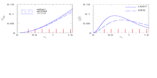
Figure 1: The parameter $\kappa_{\rm min}$ is plotted as a function of redshift $z_{s}$ in the left panel for various background cosmologies. The right panel shows the source density distribution (not normalised) for the two different surveys. The lines along the x-axis denotes the positions of the tomographic bins considered in our analysis.Notice that the parameter $k_{\rm min}$ do not depend on smoothing angular scales and only depend on the depth of the survey as well as on redshift distribution of source population. We consider two different dark energy models along with $\Lambda$CDM cosmology. The curve qCDM correspond to $w_{0}=-0.95$ and the model w0w1 correspond to an evolving dark energy model $w(x)=-1+z/(1+z)$.

In Figure (1) we plot the parameter $\kappa_{\rm min}$ as a function of redshift for different cosmologies (left panel).We also show the number distribution of source galaxies (right panel).

3 Lower Order Statistics of Tomographic Convergence Maps

Using these definitions we can compute the projected two-point correlation function in terms of the dark matter power spectrum $P_{\delta}(k,r)$ (Peebles 1980, Kaiser 1992):

$$\langle\kappa_{(i)}({\hat{\Omega}}_{1})\kappa_{(j)}({\hat{\Omega}}_{2})\rangle_{c}={\int_{0}^{r_{s}}}d{r}{\omega_{(i)}(r){\omega_{(j)}(r)}\over d^{2}_{A}(r)}\int{d^{2}{\bf l}\over(2\pi)^{2}}~{}\exp(i{\bf\theta}_{12}\cdot{\bf l})~{}{\rm P}_{\delta}{\left[{l\over d_{A}(r)},r\right]}W^{2}_{\rm TH}(l\theta_{0}).$$ (9)

Here $\theta_{12}$ is the angular separation projected onto the surface of the sky ($\cos|\theta_{12}|=\hat{\Omega}_{1}\cdot\hat{\Omega}_{2}$) and we have also introduced ${\bf l}=d_{A}(r){\bf k}_{\perp}$ to denote the scaled projected wave vector; $\omega_{i}(r)$ are the weak lensing projection weights for the ith photometric bins defined in Eq.(3); to include photometric redshift errors we simply need to use $\omega_{i}(r)$ defined in Eq.(4). Using Limber’s approximation (Limber, 1954) the variance of $\kappa_{(i)}(\theta_{0})$ smoothed using a top-hat window $W_{\rm TH}(\theta_{0})$ with a radius $\theta_{0}$ can be written as:

$$\langle\kappa_{(i)}^{2}\rangle={\int_{0}^{r_{s}}}d{r}{\omega_{(i)}^{2}(r)\over d_{A}^{2}(r)}\int{d^{2}{\bf l}\over(2\pi)^{2}}~{}{\rm P}_{\delta}{\Big{(}{l\over d_{\rm A}(r)},r\Big{)}}W_{\rm TH}^{2}(l\theta_{0}).$$ (10)

The variance is plotted for different redshift bins in Figure (2). Similarly the higher order moments of the smoothed temperature field relate $\langle\kappa^{p}({\theta_{0}})\rangle$ to the 3-dimensional multi-spectra of the underlying dark matter distribution $B_{p}$ (Hui 1999, Munshi & Coles 2000):

$$\langle\kappa_{(i)}^{3}\rangle_{c}={\int_{0}^{r_{s}}}dr{\omega_{(i)}^{3}(r)\over d_{\rm A}^{6}(r)}\int{d^{2}{\bf l}_{1}\over(2\pi)^{2}}W_{\rm TH}(l_{1}\theta_{0})\int{d^{2}{\bf l_{2}}\over(2\pi)^{2}}W_{\rm TH}(l_{2}\theta_{0})\int{d^{2}{\bf l}_{3}\over(2\pi)^{3}}W_{\rm TH}(l_{3}\theta_{0})~{}{\rm B}_{\delta}\Big{(}{l_{1}\over d_{A}(r)},{l_{2}\over d_{A}(r)},{l_{3}\over d_{\rm A}(r)},r\Big{)}_{\sum{\bf l}_{i}=0}$$ (11)

$$\langle\kappa_{(i)}^{4}\rangle_{c}={\int_{0}^{r_{s}}}d{r}{\omega^{2}_{(i)}(r)\omega^{2}_{(j)}(r)\over d_{\rm A}^{8}(r)}\int{d^{2}{\bf l}_{1}\over(2\pi)^{2}}{\rm W}_{\rm TH}(l_{1}\theta_{0})\int{d^{2}{\bf l_{2}}\over(2\pi)^{2}}{\rm W}_{\rm TH}(l_{2}\theta_{0})\int{d^{2}{\bf l}_{3}\over(2\pi)^{2}}{\rm W}_{\rm TH}(l_{3}\theta_{0})\int{d^{2}{\bf l}_{4}\over(2\pi)^{2}}{\rm W}_{\rm TH}(l_{4}\theta_{0}){}$$

$$\quad\quad\quad\quad\quad\quad~{}\times{\rm T}_{\delta}\Big{(}{l_{1}\over d_{A}(r)},{l_{2}\over d_{A}(r)},{l_{3}\over d_{\rm A}(r)},{l_{4}\over d_{\rm A}(r)},r\Big{)}_{\sum{\bf l}_{i}=0}.$$ (12)

The subscripts $\sum{\bf l}_{i}=0$ represent the delta function $\delta_{\rm D}(\sum l_{i})$. We will use these results to show that it is possible to compute the complete probability distribution function of $\kappa_{(i)}$ from the underlying dark matter probability distribution function. Details of the analytical results presented here can be found in (Munshi & Coles, 2000). A similar analysis for the higher order cumulant correlators of the smoothed convergence field relating $\kappa_{(i)}^{p}({\hat{\Omega}}_{1})\kappa_{(j)}^{q}({\hat{\Omega}}_{2})\rangle_{c}$ with multi-spectra of underlying dark matter distribution $B_{p+q}$ can be expressed as (Szapudi & Szalay, 1997; Munshi & Coles, 2000, 2002):

$$\langle\kappa_{(i)}^{2}({\hat{\Omega}}_{1})\kappa_{(j)}({\hat{\Omega}}_{2})\rangle_{c}=\int_{0}^{r_{s}}{\omega_{(i)}^{2}(r)\omega_{(j)}(r)\over d_{\rm A}^{6}(r)}dr\int\frac{d^{2}{\bf l}_{1}}{(2\pi)^{2}}\int\frac{d^{2}{\bf l}_{2}}{(2\pi)^{2}}\int\frac{d^{2}{\bf l}_{3}}{(2\pi)^{2}}{\rm W}_{\rm TH}(l_{1}\theta_{0}){\rm W}_{\rm TH}(l_{2}\theta_{0}){\rm W}_{\rm TH}(l_{3}\theta_{0}){}$$

$$\quad\quad\quad\quad\quad\quad\quad\quad\times\exp(i{\bf\theta}_{12}\cdot{\bf l}_{3}){\rm B}_{\delta}\Big{(}{l_{1}\over d_{\rm A}(r)},{l_{2}\over d_{\rm A}(r)},{l_{3}\over d_{\rm A}(r)},r\Big{)}_{\sum{\bf l}_{i}=0}.$$ (13)

We will use and extend these results in this paper to show that it is possible to compute the whole bias function $b(>\kappa)$, i.e. the bias associated with those spots in convergence map which $\kappa$ is above certain threshold (which acts as a generating function for these cumulant correlators) from the statistics of underlying over-dense dark objects (Munshi, Coles & Melott, 1999a, b).

4 Hierarchical Ansatze

The spatial length scales corresponding to small angles are in the highly non-linear regime of gravitational clustering. Assuming a ”tree” model for the matter correlation hierarchy in the highly non-linear regime, one can write the general form of the $N$th order correlation function $\xi^{(p)}_{\delta}$ as (Peebles 1980, Bernardeau & Schaeffer 1992, Szapudi & Szalay 1993):

$$\xi^{(3)}_{\delta}({\bf r}_{1},{\bf r}_{2},{\bf r}_{3})=Q_{3}(\xi_{\delta}^{(2)}({\bf r}_{1},{\bf r}_{2})\xi_{\delta}^{(2)}({\bf r}_{1},{\bf r}_{3})+{\rm cyc.perm.});$$ (14)

$$\xi^{(4)}_{\delta}({\bf r}_{1},\cdots,{\bf r}_{4})=R_{a}(\xi_{\delta}^{(2)}({\bf r}_{1},{\bf r}_{2})\xi_{\delta}^{(2)}({\bf r}_{1},{\bf r}_{3})\xi_{\delta}^{(2)}({\bf r}_{1},{\bf r}_{4})+{\rm cyc.perm.})+R_{b}(\xi_{\delta}^{(2)}({\bf r}_{1},{\bf r}_{2})\xi_{\delta}^{2}({\bf r}_{2},{\bf r}_{3})\xi_{\delta}^{(2)}({\bf r}_{3},{\bf r}_{4})+{\rm cyc.perm.}).$$ (15)

In general for correlation functions of arbitrary order are constructed by taking a sum over all possible topologies with respective amplitudes parameters $Q_{N,\alpha}$, which in general will be different:

$$\xi^{({\rm p})}_{\delta}({\bf r}_{1},\dots\bf r_{\rm p})=\sum_{\alpha,\rm p-trees}Q_{p,\alpha}\sum_{\rm labellings}\prod_{\rm edges}^{(\rm p-1)}\xi^{(2)}_{\delta}({\bf r}_{i},{\bf r}_{j}).$$ (16)

To simplify the notation we will use $\xi^{(2)}_{\delta}(r_{1},r_{2})\equiv\xi_{12}$ and $\bar{\xi}_{2}$ for its volume average over a volume $v$. It is interesting to note that a similar hierarchy develops in the quasi-linear regime in the limit of vanishing variance (Bernardeau 1992); however the hierarchical amplitudes $Q_{p,\alpha}$ become shape dependent functions in the quasilinear regime. In the highly nonlinear regime there are some indications that these functions become independent of shape, as suggested by studies of the lowest order parameter $Q_{3}=Q$ using high resolution numerical simulations (Sccocimarro et al. 1998). In Fourier space such an ansatz means that the hierarchy of multi-spectra can be written as sums of products of the matter power-spectrum:

$${\rm B}^{(3)}_{\delta}({\bf k}_{1},{\bf k}_{2},{\bf k}_{3})_{\sum k_{i}=0}=Q_{3}(P_{\delta}({\bf k}_{1})P_{\delta}({\bf k}_{2})+P_{\delta}({\bf k}_{2})P_{\delta}({\bf k}_{3})+P_{\delta}({\bf k}_{3})P_{\delta}({\bf k}_{1}));$$ (17)

$${\rm B}^{(4)}_{\delta}({\bf k}_{1},{\bf k}_{2},{\bf k}_{3},{\bf k}_{4})_{\sum k_{i}=0}=R_{a}\ P_{\delta}({\bf k}_{1})P_{\delta}({\bf k}_{1}+{\bf k}_{2})P_{\delta}({\bf k}_{1}+{\bf k}_{2}+{\bf k}_{3})+{\rm cyc.perm.}+R_{b}(\ P_{\delta}({\bf k}_{1})P_{\delta}({\bf k}_{2})P_{\delta}({\bf k}_{3})+{\rm cyc.perm.}$$ (18)

In general for p-the order poly-spectra $B^{(p)}_{\delta}({\bf k_{1}},\dots\bf k_{p})$ we can write:

$${\rm B}^{({\rm p})}_{\delta}({\bf k}_{1},\dots\bf k_{\rm p})=\sum_{\alpha,\rm p-trees}Q_{{\rm p},\alpha}\sum_{\rm labellings}\prod_{\rm edges}^{(p-1)}P_{\delta}({\bf k}_{i},{\bf k}_{j}).$$ (19)

Different hierarchical models differ in the way they predict the amplitudes of different tree topologies. Bernardeau & Schaeffer (1992) considered the case where amplitudes in general are factorisable, at each order one has a new “star” amplitude and higher order “snake” and “hybrid” amplitudes can be constructed from lower order “star” amplitudes (see Munshi, Melott & Coles 1999a,b,c for a detailed description). In models proposed by Szapudi & Szalay (1993) it was assumed that all hierarchical amplitudes of any given order are degenerate. Galaxy surveys have been used to study these ansatze. Our goal here is to show that weak-lensing surveys can also provide valuable information in this direction, in addition to constraining the matter power-spectra and background geometry of the universe. We will use the model proposed by Bernardeau & Schaeffer (1992) and its generalization to the quasi-linear regime by Bernardeau (1992, 1994) to construct the PDF of the weak lensing field $\kappa_{(i)}$. We express the one-point cumulants as:

$$\langle\kappa_{(i)}^{3}\rangle_{c}=(3Q_{3}){\cal C}^{(i)}_{3}[\kappa^{2}_{\theta_{0}}]=S_{3}^{(i)}\langle\kappa_{(i)}^{2}\rangle_{c}^{2}\quad\quad\langle\kappa_{(i)}^{4}\rangle_{c}=(12R_{a}+4R_{b}){\cal C}^{(i)}_{4}[\kappa^{3}_{\theta_{0}}]=S_{4}^{(i)}\langle\kappa_{(i)}^{2}\rangle_{c}^{3},$$ (20)

where we have introduced the following notation:

$${\cal C}^{ij}_{p+q}[[{\cal J}_{\theta_{0}}(r)]^{p+q-2}[{\cal J}_{\theta_{12}}(r)]]=\int_{0}^{r_{s}}{\omega_{(i)}^{p}(r)\omega_{(j)}^{q}(r)\over d_{A}^{2(p+q-1)}(r)}[{\cal J}_{\theta_{0}}(r)]^{p+q-2}[{\cal J}_{\theta_{12}}(r)]dr;$$ (21)

$$[{\cal J}_{\theta_{0}}(r)]\equiv\int\frac{d^{2}\bf l}{(2\pi)^{2}}P_{\delta}\left({l\over d_{\rm A}(r)}\right){\rm W}_{\rm TH}^{2}(l\theta_{0}).\quad\quad[{\cal J}_{\theta_{12}}(r)]\equiv\int\frac{d^{2}\bf l}{(2\pi)^{2}}P_{\delta}\left({l\over d_{\rm A}(r)}\right){\rm W}_{\rm TH}^{2}(l\theta_{0})\exp({\bf l}\cdot{\bf\theta_{12}}).$$ (22)

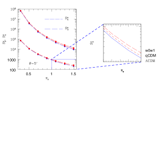
Figure 3: The skewness parameter $S^{\kappa}_{3}$ and the kurtosis parameter $S^{\kappa}_{4}$ is plotted for different redshift bins. Three different cosmologies are displayed as before.

The normalised cumulants for convergence in the i-th bin are denoted by (skewness) $S_{3}^{(i)}$ and (kurtosis) $S_{4}^{(i)}$ and are plotted in Figure (3). Eq.(20) was derived by Hui (1998) in the context of weak lensing surveys. He showed that his result agrees well with the ray tracing simulations of Jain, Seljak and White (1998). Later studies extended this result to the entire family of two-point statistics such as cumulant correlators (Munshi & Coles 1999, Munshi & Jain 1999).

$$\langle\kappa_{(i)}^{2}({\hat{\Omega}}_{1})\kappa_{(j)}({\hat{\Omega}}_{2})\rangle_{c} = 2Q_{3}{\cal C}_{3}^{(ij)}[{\cal J}_{\theta_{0}}(r){\cal J}_{\theta_{12}}(r)]=C_{21}^{\eta}{\cal C}_{3}^{(ij)}[{\cal J}_{\theta_{0}}(r){\cal J}_{\theta_{12}}(r)]\equiv C_{21}^{(ij)}\langle\kappa_{(i)}^{2}\rangle_{c}\langle\kappa_{(i)}({\hat{\Omega}}_{1})\kappa_{(j)}({\hat{\Omega}}_{2})\rangle_{c},$$ (23)

$$\langle\kappa_{(i)}^{3}({\hat{\Omega}}_{1})\kappa_{(j)}({\hat{\Omega}}_{2})\rangle_{c} = (3R_{a}+6R_{b}){\cal C}_{4}^{(ij)}[{\cal J}_{\theta_{0}}(r){\cal J}_{\theta_{12}}(r)]=C_{31}^{\eta}{\cal C}_{4}^{(ij)}[{\cal J}_{\theta_{0}}(r)^{2}{\cal J}_{\theta_{12}}(r)]\equiv C_{(31)}^{(ij)}\langle\kappa_{(i)}^{2}\rangle_{c}^{2}\langle\kappa_{(i)}({\hat{\Omega}}_{1})\kappa_{j}({\hat{\Omega}}_{2})\rangle_{c},$$ (24)

$$\langle\kappa_{(i)}^{2}({\hat{\Omega}}_{1})\kappa_{(j)}^{2}({\hat{\Omega}}_{2})\rangle_{c} = 4R_{b}{\cal C}_{4}^{(ij)}[{\cal J}_{\theta_{0}}(r)^{2}{\cal J}_{\theta_{12}}(r)]=C_{(22)}^{\eta}{\cal C}_{4}^{(ij)}[{\cal J}_{\theta_{0}}(r)^{2}{\cal J}_{\theta_{12}}(r)]\equiv C_{22}^{(ij)}\langle\kappa_{(i)}^{2}\rangle_{c}\langle\kappa_{(j)}^{2}\rangle_{c}\langle\kappa_{(i)}({\hat{\Omega}}_{1})\kappa_{(j)}({\hat{\Omega}}_{2})\rangle_{c},$$ (25)

$$\langle\kappa_{(i)}^{4}({\hat{\Omega}}_{1})\kappa_{(j)}({\hat{\Omega}}_{2})\rangle_{c} = (24S_{a}+36S_{b}+4S_{c}){\cal C}_{5}^{(ij)}[{\cal J}_{\theta_{0}}(r)^{3}{\cal J}_{\theta_{12}}(r)]=C_{41}^{\eta}{\cal C}_{5}^{(ij)}[{\cal J}_{\theta_{0}}(r)^{3}{\cal J}_{\theta_{12}}(r)]\equiv C_{41}^{(ij)}\langle\kappa_{(i)}^{2}\rangle_{c}^{3}\langle\kappa_{(i)}({\hat{\Omega}}_{1})\kappa_{(j)}({\hat{\Omega}}_{2})\rangle_{c},$$ (26)

$$\langle\kappa_{(i)}^{3}({\hat{\Omega}}_{1})\kappa_{(j)}^{2}({\hat{\Omega}}_{2})\rangle_{c} = (12S_{a}+6S_{b}){\cal C}_{5}^{(ij)}[{\cal J}_{\theta_{0}}(r)^{3}{\cal J}_{\theta_{12}}(r)]=C_{32}^{\eta}{\cal C}_{5}[{\cal J}_{\theta_{0}}(r)^{3}{\cal J}_{\theta_{12}}(r)]\equiv C_{32}^{(ij)}\langle\kappa_{(i)}^{2}\rangle_{c}^{2}\langle\kappa_{(j)}^{2}\rangle_{c}\langle\kappa_{(i)}({\hat{\Omega}}_{1})\kappa_{(j)}({\hat{\Omega}}_{2})\rangle_{c}.$$ (27)

where $C_{pq}^{\eta}$ denotes the cumulant correlators for the underlying mass distribution. These results essentially employ the small angle approximation or Limber’s approximation (Limber, 1954) that are routinely used in computation of higher order cumulants in many cosmological contexts. Other approximations such as the Born approximation that we use have been verified by testing against simulations.

In a related, but slightly different context, these lower order statistics can also be helpful in probing the pressure bias as a function of scale for the study of thermal Sunyaev-Zel’dovich (tSZ) effect or its cross-correlation against tomographic weak lensing maps (Munshi et al., 2011b). The thermal Sunyaev-Zel’dovich effect probes the line-of-sight integral of electronic pressure fluctuations. Cross-correlating (frequency-cleaned) $y$ maps from ongoing CMB experiments such as Planck (Planck Collaboration, 2006) against the weak lensing tomographic maps can provide a redshift resolved picture of reionization history of the Universe. The signal-to-noise will however decrease with increasing order of these statistics. Indeed the study of PDF or bias that we undertake next will essentially combine information from all orders.

In Figure (2) and Figure (3) we have plotted the variance and the lower order $S_{p}$ parameters respectively as a function of smoothing scale $\theta_{0}$.

5 The Generating Function

In a scaling analysis of the count probability distribution function (CPDF) the void probability distribution function (VPF) plays a fundamental role. It can be related to the generating function of the cumulants or $S_{p}$ parameters, $\phi(y)$ (White 1979, Balian & Schaeffer 1989) :

$$P_{v}(0)=\exp(-\bar{N}\sigma(N_{c}))=\exp\Big{(}-{\phi(N_{c})\over\bar{\xi}_{2}}\Big{)}.$$ (28)

Where $P_{v}(0)$ is the probability of having no “particles” in a cell of of volume $v$, $\bar{N}$ is the average occupancy of these “cells”, and $N_{c}=\bar{N}{\bar{\xi}}_{2}$. All statistical quantities correspond to underlying density contrast $\delta$. The VPF $P_{v}(0)$ is a special case of the count probability distribution function (CPDF) $P_{v}(N)$. The VPF $P_{v}(0)$ contains information of the entire CPDF $P_{v}(N)$

The VPF is meaningful only for a discrete distribution of particles and can’t be defined for smooth density fields such as $\delta$ or $\kappa(\theta_{0})$. However the scaling functions $\sigma(y)$ and $\phi(y)$, defined above in Eq.(28), $\sigma(y)=-{\phi(y)/y}$, are very useful even for continuous distributions where they can be used as a generating function of one-point cumulants or $S_{p}$ parameters: $\phi(y)=\sum_{p=1}^{\infty}{S^{\delta}_{p}/p!}y^{p}$. The function $\phi(y)$ satisfies the constraint $S^{\delta}_{1}=S^{\delta}_{2}=1$ necessary for proper normalization of PDF. The other generating function which plays a very important role in such analysis is the generating function for the vertex amplitudes $\nu_{n}$ associated with nodes appearing in the tree representation of higher order correlation hierarchy ($Q_{3}=\nu_{2}$, $R_{a}=\nu_{2}^{2}$ and $R_{b}=\nu_{3}$). In practice it is possible to work with a perturbative expansion of the vertex generating function ${\cal G}(\tau)$. In terms of the vertices this is defined as: ${\cal G}(\tau)=\sum_{n=0}^{\infty}(-1)^{n}{\nu_{n}/n!}$. However in the highly nonlinear regime a closed form is used. A more specific model for ${\cal G}(\tau)$, which is useful to make more specific predictions (Bernardeau & Schaeffer 1979) is given by ${\cal G}(\tau)=\Big{(}1+{\tau/\kappa_{a}}\Big{)}^{-\kappa_{a}}$. We will relate $\kappa_{a}$ with other parameters of scaling models. While the definition of VPF does not involve any specific form of hierarchical ansatz it is to realize that writing the tree amplitudes in terms of the weights associated with nodes is only possible when one assumes a factorisable model of the tree hierarchy (Bernardeau & Schaeffer 1992) and other possibilities which do not violate the tree models are indeed possible too (Bernardeau & Schaeffer 1999). The generating functions for tree nodes can be related to the VPF by solving a pair of implicit equations (Balian & Schaeffer 1989),

$$\phi(y)=y{\cal G}(\tau)-{1\over 2}y{\tau}{d\over d\tau}{\cal G}(\tau);\quad\quad\tau=-y{d\over d\tau}{\cal G}(\tau).$$ (29)

The above description has been limited to the level of constructing one-point PDF. A more detailed analysis is needed to include the effect of correlation between two or more correlated volume element which will provide information about bias and cumulant correlators. The bias $b(\delta)$ can be introduced the following expression for the joint or two-point PDF:

$$p(\delta_{1},\delta_{2})d\delta_{1}d\delta_{2}=p(\delta_{1})p(\delta_{2})(1+b(\delta_{1})\xi_{12}b(\delta_{2}))d\delta_{1}d\delta_{2}$$ (30)

The function $\tau(y)$ - sometimes denoted by $\beta(y)$ in the literature - plays the role of a generating function for the factorized cumulant correlators $C^{\eta}_{p1}$ ($C^{\eta}_{pq}=C^{\eta}_{p1}C^{\eta}_{q1}$) (Bernardeau & Schaeffer, 1992; Bernardeau, 1992, 1994): $\tau(y)=\sum_{p=1}^{\infty}y^{p}{C^{\eta}_{p1}/p!}$. We will next consider two different regimes; the quasilinear regime valid at large angular scales and the highly nonlinear regime valid at smaller angular scales.

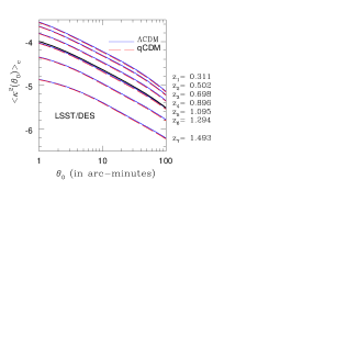
Figure 2: The plots shows the variance in convergence $\langle\kappa^{2}(\theta_{0})\rangle_{c}$ as a function of smoothing angular scales $\theta_{0}$. A top-hat window has been assumed. The curves from top to bottom correspond to various tomographic bins. The redshift bins correspond to $\Delta z_{s}=0.2$ and covers a range $z_{s}=0.2-1.4$.The curve qCDM correspond to $w_{0}=-0.95$. The higher curves correspond to the deeper redshift bins. See text for more details.

5.1 The Highly Non-linear Regime

bb The PDF $p(\delta)$ and bias $b(\delta)$ can be related to their generating functions VPF $\phi(y)$ and $\tau(y)$ respectively by following equations (Balian & Schaeffer 1989, Bernardeau & Schaeffer 1992, Bernardeau & Schaeffer 1999),

$$p(\delta)=\int_{-i\infty}^{i\infty}{dy\over 2\pi i}\exp\Big{[}{(1+\delta)y-\phi(y)\over\bar{\xi}_{2}}\Big{]};\quad b(\delta)p(\delta)=\int_{-i\infty}^{i\infty}{dy\over 2\pi i}\tau(y)\exp\Big{[}{(1+\delta)y-\phi(y)\over\bar{\xi}_{2}}\Big{]}.$$ (31)

The function $\phi(y)$ ($\tau(y)$) plays an important role in any calculation involving hierarchical ansatz because it completely determines the behavior of the PDF $p(\delta)$ (bias $b(\delta)$ ) for all values of $\delta$. The different asymptotic expressions of $\phi(y)$ govern the behavior of $p(\delta)$ for different intervals of $\delta$. For large $y$ we can express $\phi(y)$ as: $\phi(y)=ay^{1-\omega}$. No theoretical analysis has been done so far to link the newly introduced parameter $\omega$ and the initial power spectral index $n$. In the highly nonlinear regime, numerical simulations are generally used to fix $\omega$ for a specific initial condition. (Colombi et. al. (1992, 1994, 1995), Munshi et al (1999)). Typically for a power law initial power spectrum with pictorial index $n=-2$ one obtains $\omega=0.3$. The VPF $\phi(y)$ and its two-point analog $\tau(y)$ both exhibit singularity for small but negative value of $y_{s}$,

$$\phi(y)=\phi_{s}-a_{s}\Gamma(\omega_{s})(y-y_{s})^{-\omega_{s}};\quad\quad\tau(y)=\tau_{s}-b_{s}(y-y_{s})^{-\omega_{s}-1}.$$ (32)

For the factorisable model of the hierarchical clustering the parameter $\omega_{s}$ takes the value $-3/2$ and $a_{s}$ and $b_{s}$ can be expressed in terms of the nature of the generating function ${\cal G}(\tau)$ and its derivatives near the singularity $\tau_{s}$ (Bernardeau & Schaeffer 1992):

$$a_{s}={1\over\Gamma(-1/2)}{\cal G}^{\prime}(\tau_{s}){\cal G}^{\prime\prime}(\tau_{s})\left[{2{\cal G}^{\prime}(\tau_{s}){\cal G}^{\prime\prime}(\tau_{s})\over{\cal G}^{\prime\prime\prime}(\tau_{s})}\right]^{3/2};\quad\quad b_{s}=\left[{2{\cal G}^{\prime}(\tau_{s}){\cal G}^{\prime\prime}(\tau_{s})\over{\cal G}^{\prime\prime\prime}(\tau_{s})}\right]^{1/2}.$$ (33)

As mentioned before the parameter $k_{a}$ which we have introduced in the definition of ${\cal G}(\tau)$ can be related to the parameters $a$ and $\omega$ appearing in the asymptotic expressions of $\phi(y)$ (Balian & Schaeffer 1989, Bernardeau & Schaeffer 1992),

$$\omega=k_{a}/(k_{a}+2),;\quad\quad a={k_{a}+2\over 2}k_{a}^{k_{a}/k_{a}+2}.$$ (34)

Similarly the parameter $y_{s}$ which describes the behavior of the function $\phi(y)$ near its singularity can be related to the behavior of ${\cal G(\tau)}$ near $\tau_{s}$ which is the solution of the equation (Balian & Schaeffer 1989, Bernardeau & Schaeffer 1992), $\tau_{s}={{\cal G}^{\prime}(\tau_{s})/{\cal G}^{\prime\prime}(\tau_{s})}$, finally we can relate $k_{a}$ to $y_{s}$ by following expression (see eq. (34)): $y_{s}=-{\tau_{s}/{\cal G}^{\prime}(\tau_{s})}$, or we can write:

$$-{1\over y_{s}}=x_{\star}={1\over k_{a}}{(k_{a}+2)^{k_{a}+2}\over(k_{a}+1)^{k_{a}+1}}.$$ (35)

The newly introduced variable $x_{\star}$ will be useful to define the large $\delta$ tail of the PDF $p(\delta)$ and the bias $b(\delta)$. The asymptotes of $\phi(y)$ are linked with the behavior of $p(\delta)$ for various regimes of $\delta$. For very large values of the variance $\bar{\xi}_{2}$ it is possible to define a scaling function $p(\delta)={h(x)/\bar{x}i_{2}^{2}}$ which will encode the scaling behavior of the PDF, where $x$ plays the role of the scaling variable and is defined as $x={(1+\delta)}/\bar{\xi}_{2}$. We list below different ranges of $\delta$ and specify the behavior of $p(\delta)$ and $b(\delta)$ in these regimes (Balian & Schaeffer 1989).

$${\bar{\xi}}^{-\omega/(1-\omega)}\gg 1+\delta\gg\bar{\xi};~{}~{}~{}~{}~{}~{}p(\delta)={a\over\bar{\xi}_{2}^{2}}{1-\omega\over\Gamma(\omega)}\Big{(}{1+\delta\over\xi_{2}}\Big{)}^{\omega-2};~{}~{}~{}~{}~{}b(\delta)=\left({\omega\over 2a}\right)^{1/2}{\Gamma(\omega)\over\Gamma[{1\over 2}(1+\omega)]}\left({1+\delta\over\bar{\xi}_{2}}\right)^{(1-\omega)/2}$$ (36)

$$1+\delta\gg{\bar{\xi}}_{2};~{}~{}~{}~{}p(\delta)={a_{s}\over\bar{\xi}_{2}^{2}}\Big{(}{1+\delta\over\bar{\xi}_{2}}\Big{)}\exp\Big{(}-{1+\delta\over x_{\star}\bar{\xi}_{2}}\Big{)};~{}~{}~{}~{}~{}b(\delta)=-{1\over{\cal G}^{\prime}(\tau_{s})}{(1+\delta)\over{{\bar{\xi}}_{2}}}$$ (37)

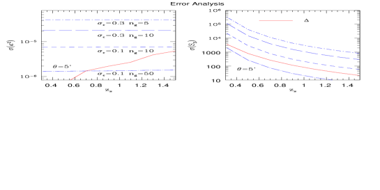
Figure 4: The left panel shows the $1\sigma$ error in estimation of the variance $\langle\kappa^{2}\rangle_{\rm c}$ and the right panel shows the error of estimation in the skewness paramter $S_{3}$ as a function of tomographic redshift. The angular scale is fixed at $\theta_{s}=5^{\prime}$. Various curves correspond to a choice of the intrinsic ellipticity distribution of galaxies $\sigma_{\epsilon}$ and number of galaxies $n_{g}$ (=number of galaxies/arcmin²) are as depicted. The solid lines are the difference between the $\Lambda$CDM model and the qCDM model. The scatter is computed using the formalism developed in (Valageas, Munshi & Barber, 2005).

The integral constraints satisfied by scaling function $h(x)$ are $S^{\eta}_{1}=\int_{0}^{\infty}xh(x)dx=1$ and $S^{\eta}_{2}=\int_{0}^{\infty}x^{2}h(x)dx=1$. These take care of normalization of the function $p(\delta)$. Similarly the normalization constraint over $b(\delta)$ or equivalently $b(x)$ can be expressed as $C^{\eta}_{11}=\int_{0}^{\infty}xb(x)h(x)dx=1$, which translates into $\int_{-1}^{\infty}d\delta b(\delta)p(\delta)=0$ and $\int_{-1}^{\infty}d\delta b(\delta)p(\delta)=1$. Several numerical studies have produced the behavior of $h(x)$ and $b(x)$ for different initial conditions (e.g. Colombi et al. 1992,1994,1995; Munshi et al. 1999, Valageas et al. 1999). For very small values of $\delta$ the behavior of $p(\delta)$ is determined by the asymptotic behavior of $\phi(y)$ for large values of $y$, and it is possible to define another scaling function $g(z)$ which is completely determined by $\omega$, the scaling parameter can be expressed as $z=(1+\delta)a^{-1/(1-\omega)}{\bar{\xi}}_{2}^{\omega/(1-\omega)}$. However numerically it is much easier to determine $\omega$ from the study of $\sigma(y)$ compared to the study of $g(z)$ (e.g. Bouchet & Hernquist 1992).

$$1+\delta\ll\bar{\xi}_{2};~{}~{}~{}~{}p(\delta)=a^{-1/(1-\omega)}[{\bar{\xi}}_{2}]^{\omega/(1-\omega)}\sqrt{(1-\omega)^{1/\omega}\over 2\pi\omega z^{(1+\omega)/\omega}}\exp\Big{[}-\omega\Big{(}{z\over 1-\omega}\Big{)}^{-{{1-\omega}\over\omega}}\Big{]};~{}~{}~{}~{}~{}~{}~{}b(\delta)=-\left({2\omega\over\bar{\xi}_{2}}\right)^{1/2}\left({1-\omega\over z}\right)^{(1-\omega)/2\omega}$$ (38)

To summarize, the entire behaviour of the PDF $p(\delta)$ and bias $b(\delta)$ are encoded in two different scaling functions, $h(x)$ and $g(z)$. These scaling functions are relevant for small and large $\delta$ behavior of the function $p(\delta)$ and $b(\delta)$. Typically the PDF $p(\delta)$ shows a cutoff at both large and small values of $\delta$ and it exhibits a power-law in the middle. The power law behavior is prominent in highly non-linear regime. With the decrease in $\bar{\xi}_{2}$ the range of $\delta$ for which $p(\delta)$ shows such a power law behavior decreases finally to vanish for the case of very small variance i.e. in the quasi-linear regime. Similarly the bias is a very small and slowly varying function for moderately over dense objects but increases rapidly for over-dense objects. These deductions are in qualitative agreement with results from the halo model based approaches.

5.2 The Quasi-linear Regime

The Generating function formalism was used by (Bernardeau, 1992, 1994) in the quasilinear regime. Unlike highly nonlinear regime the quasilinear regime can be dealt with using perturbative analysis. This particular analysis assumes the variance of the smoothed density contrast is smaller than unity. The generating function formalism was use to construct the PDF and bias using the tree-level perturbation theory to arbitrary order. In this regime the scaling parameters $\omega$ and $k_{a}$ can be expressed in terms of the initial power spectral index $n$. In general the numerical values of the parameters $k_{a}$ or $\omega$ characterizing VPF or CPDF are different from there highly non-linear values. The PDF and bias now can be expressed in terms of $G_{\delta}(\tau)$ (Bernardeau 1992; Bernardeau 1994):

$$p(\delta)d\delta={1\over-{\cal G}_{\delta}^{\prime}(\tau)}\Big{[}{1-\tau{\cal G}_{\delta}^{\prime\prime}(\tau)/{\cal G}_{\delta}^{\prime}(\tau)\over 2\pi{\bar{\xi}}_{2}}\Big{]}^{1/2}\exp\Big{(}-{\tau^{2}\over 2{\bar{\xi}}_{2}}\Big{)}d\tau;~{}~{}~{}~{}~{}b(\delta)=-\left({k_{a}\over\bar{\xi}_{2}}\right)\left[(1+{\cal G}_{\delta}(\tau))^{1/k_{a}}-1\right],$$ (39)

$${\cal G}_{\delta}(\tau)={\cal G}(\tau)-1=\delta.$$ (40)

The above expression is valid for $\delta<\delta_{c}$ where the $\delta_{c}$ is the value of $\delta$ which cancels the numerator of the pre-factor of the exponential function appearing in the above expression. For $\delta>\delta_{c}$ the PDF develops an exponential tail which is related to the presence of singularity in $\phi(y)$ in a very similar way as in the case of its highly non-linear counterpart (Bernardeau 1992; Bernardeau 1994).

$$p(\delta)d\delta={3a_{s}\sqrt{{\bar{\xi}}_{2}}\over 4{\sqrt{\pi}}}\delta^{-5/2}\exp\Big{[}-|y_{s}|{\delta\over{\bar{\xi}}_{2}}+{|\phi_{s}|\over{\bar{\xi}}_{2}}\Big{]}d\delta;~{}~{}~{}~{}~{}b(\delta)=-{1\over{\cal G}^{\prime}(\tau_{s})}{(1+\delta)\over{{\bar{\xi}}_{2}}}$$ (41)

These expressions were used by Munshi & Jain (2001, 2000) and Valageas (2000) for the construction of weak lensing PDF in projection. The bias was studied in (Munshi, 2000) for projected surveys. The tests against numerical simulations show remarkable agreement for a range of angular scales. Later studies refined these results as well as incorporated various different smoothing windows (Munshi, Valageas & Barber, 2004; Valageas, Munshi & Barber, 2005). We extend these results derived for surveys in projection to tomographic surveys in this paper.

It is worth mentioning that, there have been various attempts to extend the perturbative results to the highly nonlinear regime (see e.g. (Colombi et al., 1997; Valageas & Munshi, 2004))

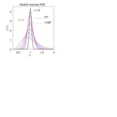
Figure 5: The PDF $p(\eta)$ of the reduced convergence $\eta$ as a function $\eta=1+\delta$. The plots with decreasing peak height correspond to lower redshift bins. Two different approximations are being compared. The solid line correspond to the lognormal approximation and the dashed line correspond to the perturbative calculations. The results are shown for a smoothing angular scale $\theta_{s}=5^{\prime}$.

6 The Lognormal Distribution

An alternative to the hierarchical ansatz, the lognormal distribution, for the description of the matter PDF which has long been known as a successful empirical prescription for the characterization of the dark matter distribution as well as the observed galaxy distribution (Hamilton, 1985; Coles & Jones, 1991; Bouchet et al, 1993; Kofman et al., 1994). Detailed discussion for comparison of lognormal distribution and the perturbative calculations can be found in (Bernardeau & Kofman, 1995). The lognormal distribution was further generalized to the skewed-lognormal distribution (Colombi, 1994). In general a variable might be modelled as lognormal if it can be thought of as the multiplicative product of many independent random variables.

Although inherently local in nature, the lognormal distribution can provide a good fit to both one-point PDF and its generalisation to compute its two-point analog and hence the bias (Taruya et al., 2002). The one- and two-point lognormal PDF can be expressed as (Kayo, Taruya, Suto, 2001):

$$p_{\rm ln}(\delta)d\delta={1\over\sqrt{2\pi\bar{\Sigma}}}\exp\left[-{\Delta^{2}\over 2\Sigma^{2}}\right]{d\delta\over 1+\delta};\quad\quad\Sigma^{2}=\ln(1+\sigma^{2});\quad\quad\Delta=\ln[(1+\delta)\sqrt{(1+\sigma^{2})};$$ (42)

$$p_{\rm ln}(\delta_{1},\delta_{2})d\delta_{1}d\delta_{2}={1\over 2\pi\sqrt{\Sigma^{2}-X_{12}^{2}}}\exp\left[-{\Sigma(\Delta_{1}^{2}+\Delta_{2}^{2})-2X_{12}\Delta_{1}\Delta_{2}\over 2(\Sigma^{2}-X_{12}^{2})}\right]{d\delta_{1}\over 1+\delta_{1}}{d\delta_{2}\over 1+\delta_{2}};$$ (43)

$$\Delta_{i}=\ln[(1+\delta_{i})\sqrt{(1+\bar{\xi}_{2}^{2})};\quad\Sigma_{12}=\ln(1+\xi_{12})$$ (44)

In the limiting case of large separation $X_{12}\rightarrow 0$ we can write down the two point PDF

$$p_{\rm ln}(\delta_{1},\delta_{2})=p_{\rm ln}(\delta_{1})p_{\rm ln}(\delta_{2})[1+b_{\rm ln}(\delta_{1})\xi_{12}b_{\rm ln}(\delta_{2})];\quad\quad b_{\rm ln}(\delta_{i})=\Delta_{i}/\Sigma_{i}.$$ (45)

It is however easier to estimate the cumulative or integrated bias associated with objects beyond a certain density threshold $\delta_{0}$. This is defined as $b_{\rm ln}(\delta>\delta_{0})=\int_{\delta_{0}}^{\infty}p_{\rm ln}(\delta)b_{\rm ln}(\delta)d\delta/\int_{\delta_{0}}^{\infty}p_{\rm ln}(\delta)d\delta$. In the low variance limit ${\bar{\xi}}_{2}\rightarrow 0$ the usual Gaussian result is restored $b(\delta)=\delta/{\bar{\xi}}_{2}$. The parameters $\Lambda,\Lambda_{i},X_{12},\Sigma$ that we have introduced above can be expressed in terms of the two-point (non-linear) correlation function $\xi_{12}=\langle\delta_{1}\delta_{2}\rangle$ and the nonlinear variance $\sigma^{2}=\langle\delta^{2}\rangle$ of the smoothed density field. To understand the construction of lognormal distribution, we introduce a Gaussian PDF in variable $x$; $p(x)=(2\pi\Sigma^{2})^{1/2}\exp[-(x-\mu)^{2}/2\Sigma^{2}]$. With a change of variable $x=\ln(t)$ we can write down the PDF of $y$ which is a lognormal distribution $p(t)=(2\pi\Sigma^{2})^{1/2}\exp[-(\ln(t)-\mu)^{2}/2\Sigma^{2}]/t$. The extra factor of $(1/x)$ stems from the fact: $dt/t=dx$. Note that $y$ is positive definite and is often associate with $\rho/\rho_{0}=1+\delta$ which means $\langle t\rangle=1$. The moment generating function for the lognormal in terms of the mean $\mu$ and the variance $\Sigma$ has the following form: $\langle t^{n}\rangle=\exp(n\mu+n^{2}\Sigma^{2}/2)$. This however leads to the fact that if the underlying distribution of $x$ or the density is Gaussian we will have to impose the condition: $\mu=-\Sigma^{2}/2$. Here in our notation above $\Sigma$ is the variance of the underlying Gaussian field. The variance of $t$ defined as $\langle t^{2}\rangle-\langle t\rangle^{2}=\exp(\Sigma^{2})-1=\sigma^{2}$. So we can write $\Sigma^{2}=\ln(1+\sigma^{2})$. This is the result that was used above. The generalization to two-point or bi-variate PDF can be achieved following the same arguments and can be found in (Kayo, Taruya, Suto, 2001).

In contrast to the lognormal model the widely-used non-local ansatz for the evolution of the variance that was introduced by (Hamilton et al., 1985), the evolved nonlinear two-point correlation function is linked to that of the initial or linear two-point correlation at a different scale: $\bar{\xi}_{2}^{nl}(R_{\rm nl})=f_{nl}[\bar{\xi}_{2}^{lin}(R_{lin})]$. The two different length scales are related by the following expression: $R_{\rm nl}^{3}=(1+\bar{\xi}^{nl}_{2}(R_{\rm nl}))R_{lin}^{3}$. Such as an ansatz is derived using pair conservation equation. The non-linear (Eulerian) length scale $R_{\rm nl}$ is linked to the linear (Lagrangian) length scale $R_{\rm lin}$ from where the structure has collapsed. Numerical simulations are typically used for the determination of the fitting function $f_{\rm nl}$ (Peacock & Dodds, 1994). However, simpler asymptotic power-law forms exist in different regimes of gravitational clustering (Munshi & Padmanabhan, 1997).

The validity and limitations of the one-point and two-point PDFs have been studied extensively in the literature against N-body simulations. In Bernardeau (1992, 1994) it was shown that the PDF computed from the perturbation theory in a weakly nonlinear regime approaches the lognormal distribution function only when the primordial power spectrum is locally of the form $P(k)\propto k^{n_{e}}$ with the effective local spectra slope of the power spectrum $n_{e}\sim-1$. It was also shown that in the weakly nonlinear regime the lognormal distribution is equivalent to the hierarchical model with a generating function $\cal G(\tau)=\exp(-\tau)$. This leads to the following skewness and kurtosis parameters:

$$S^{\eta}_{3}=3+\sigma^{2};\quad\quad S^{\eta}_{4}=16+15\sigma^{2}+6\sigma^{4}+\sigma^{6}.$$ (46)

In general the $\sigma^{2}\rightarrow 0$ leads to $S_{p}^{\eta}=p^{p-2}$. On this basis Bernardeau & Kofman (1995) argues that the agreement of lognormal PDF with numerical simulations should be interpreted as purely accidental and the success of the lognormal model is simply related to the fact that for all scales relevant to cosmology the CDM power spectrum can be approximated with a power law with effective slope $n_{e}\approx-1$. However subsequent studies using numerical simulation it was shown by various authors that the lognormal distribution very accurately describes the cosmological distribution functions even in the nonlinear regime $\sigma\leq 4$ for a relatively high values of density contrast $\delta<100$ (see e.g. Kayo, Taruya, Suto (2001)).

There is no complete analytical description of gravitational clustering in the highly nonlinear regime. However several dynamical approximations were proposed in the past to mimic certain features of gravitational clustering neyond the weakly nonlinear clsutering. The Frozen Flow Approximation (FFA) approximation proposed by (Matarresse et al., 1992) is one such approximation. using perturbative techniques it was shown by (Munshi, Sahni, Starobinsky, 1994) that the FFA develops exactly the same generating function as the lognormal approximation in the quasilinear regime.

The error estimates for various lower order $S_{p}$ (right panel) and the variance (left-panel) are shown in Figure (4). A complete analytical formalism for calculation of error are given in Valageas, Munshi & Barber (2005). It requires the knowledge of higher order $S_{p}$ parameters. In our calculation of error the higher order $S_{p}$ parameters are modelled according to lognormal distribution. Different levels of noise as chareterized by the parameters that describe intrinsic ellipticity distribution $\epsilon$ and number density of galaxies/arcmin² or $n_{g}$ are considered.

7 The PDF and bias of smoothed redshift-resolved convergence maps

For computing the probability distribution function of the smoothed convergence field for individual tomographic maps $\kappa^{(i)}(\theta_{0})$, we will begin by constructing its associated cumulant generating function for individual tomographic bins $\Phi^{(i)}_{1+\kappa(\theta_{0})}(y)$. The construction is based on modelling of the volume-averaged higher order correlation function $\langle\kappa_{(i)}^{p}(\theta_{0})\rangle_{c}$ in terms of the matter correlation hierarchy:

$$\Phi^{(i)}_{1+{\kappa(\theta_{0})}}(y)=y+\sum_{p=2}^{\infty}{{\langle\kappa_{(i)}^{p}(\theta_{0})\rangle_{c}}\over\langle\kappa_{(i)}^{2}(\theta_{0})\rangle_{c}^{p-1}}y^{p}.$$ (47)

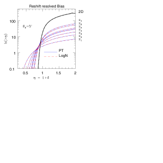
Figure 6: The cumulative bias $b(>\eta)$ of the reduced convergence $\eta=(1+\delta)$ is plotted as a function $\eta$ for various redshift bins. The smoothing angular scale is $\theta_{0}=5^{\prime}$. As before two different approximations are considered. The lognormal approximation (solid lines) and the perturbative calculations (dashed lines) reproduce nearly identical results. The curves that saturates at a higher values of cumulative bias for higher values of $\eta$ correspond to larger smoothing angular scales.

Now using the expressions for the higher moments of the convergence $\kappa(\theta_{0})$ in terms of the matter power spectrum, Eq.10 and Eq.20 gives:

$$\Phi^{(i)}_{1+{\kappa({\theta_{0}})}}(y)\equiv\sum_{p=1}{S^{(i)\kappa}_{p}\over p!}y^{p}=y+\int_{0}^{r_{s}}\sum_{p=2}^{\infty}{1\over p!}S^{\eta}_{p}{\omega_{(i)}^{p}(r)\over d_{A}(r)^{2(p-1)}(r)}\Big{[}{{\cal J}_{\theta_{0}}(r)\over\bar{\xi}_{2}^{(i)\kappa}(\theta_{0})}\Big{]}^{(p-1)}y^{p};\quad\quad\bar{\xi}_{2}^{(i)\kappa}\equiv\langle\kappa^{2}(\theta_{0})\rangle_{c}.$$ (48)

We can now use the definition of $\phi(y)$ for the matter cumulants to express $\Phi_{1+\kappa(\theta_{0})}(y)$, in terms of $\phi(y)$:

$$\Phi^{(i)}_{1+\kappa_{\theta_{0}}}(y)=\int_{0}^{r_{s}}dr\Big{[}{d_{A}^{2}(r)\bar{\xi}_{2}^{(i)\kappa}(\theta_{0})\over{\cal J}_{\theta_{0}}(r)}\Big{]}\phi\Big{[}{\omega_{(i)}(r)\over d_{A}^{2}(r)}{{\cal J}_{\theta_{0}}(r)\over\bar{\xi}_{2}^{(i)\kappa}(\theta_{0})}y\Big{]}-y\kappa_{(i)}^{\rm min};\quad\kappa^{\rm min}_{(i)}=-\int_{0}^{r_{s}}\;dr\;\omega_{(i)}(r).$$ (49)

The extra term comes from the $p=1$ term in the expansion of $\Phi_{1+\kappa(\theta_{0})}$. Note that we have used the fully non-linear generating function $\phi$ for the cumulants, though we will use it to construct a generating function in the quasi-linear regime. The analysis becomes much easier if we define a new reduced convergence field:

$$\eta_{(i)}({\theta_{0}})={{(\kappa^{\rm min}_{(i)}-\kappa_{(i)}({\theta_{0}})})/\kappa^{\rm min}_{(i)}}=1+{\kappa_{(i)}({\theta_{0}})/|\kappa^{\rm min}_{(i)}|}.$$ (50)

Here the minimum value of $\kappa_{(i)}(\theta_{0})$ i.e. $\kappa^{\rm min}_{(i)}$ occurs when the line-of-sight goes through regions that are completely empty of matter (i.e. $\delta=-1$ all along the line of sight in a redshift window that defines a specific bin i.e. Eq.(3)). While $\kappa_{(i)}({\theta_{0}})$ depends on the smoothing angle, its minimum value $\kappa^{\rm min}_{(i)}$ depends only on the source redshift and background geometry of the universe and is independent of the smoothing radius. With the reduced convergence $\eta$, the cumulant generating function is given by,

$$\Phi^{(i)}_{\eta}(y)={1\over[{\kappa^{\rm min}_{(i)}}]}\int_{0}^{r_{s}}dr\Big{[}{d_{A}^{2}(r)\over{\kappa^{\rm min}_{(i)}}}{\bar{\xi}_{2}^{(i)\kappa}(\theta_{0})\over{\cal J}_{\theta_{0}}(r)}\Big{]}\phi\Big{[}{{\kappa^{\rm min}_{(i)}}\over d_{A}^{2}(r)}{{\cal J}_{\theta_{0}}(r)\over\bar{\xi}_{2}^{(i)\kappa}(\theta_{0})}y\Big{]}.$$ (51)

The thus constructed cumulant generating function $\Phi_{\eta}(y)$ satisfies the normalization constraints $S^{\eta}_{1}=S^{\eta}_{2}=1$. The scaling function associated with $P(\eta)$ can now be easily related with the matter scaling function $h(x)$ introduced earlier:

$$h^{(i)}_{\eta}(x)=-\int_{-\infty}^{\infty}{dy\over 2\pi i}\exp(xy)\Phi^{(i)}_{\eta}(y);\quad\quad h_{\eta}^{(i)}(x)={1\over[{\kappa^{\rm min}_{(i)}}]}\int_{0}^{r_{s}}dr\Big{[}{\bar{\xi}_{2}^{(i)\kappa}(\theta_{0})\over{\cal J}_{\theta_{0}}(r){\kappa^{\rm min}_{(i)}}}\Big{]}^{2}h\Big{(}{\bar{\xi}_{2}^{(i)\kappa}(\theta_{0})x\over\omega_{(i)}(r){\cal J}_{\theta_{0}}(r){\kappa^{\rm min}_{(i)}}}\Big{)}.$$ (52)

While the expressions derived above are exact, and are derived for the most general case, using only the small angle approximation, they can be simplified considerably using further approximations. In the following we will assume that the contribution to the $r$ integrals can be replaced by an average value coming from the maximum of $\omega_{(i)}(r)$, i.e. $r_{c}$ ($0<r_{c}<r_{s}$). So we replace $\int f(r)dr$ by $1/2f(r_{c})\Delta_{r}$ where $\Delta_{r}$ is the interval of integration, and $f(r)$ is the function of comoving radial distance $r$ under consideration. Similarly we replace the $\omega(r)$ dependence in the ${\bf k}$ integrals by $\omega_{(i)}(r_{c})$.

$$|\kappa_{(i)}^{\rm min}|\approx{1\over 2}r_{s}\omega_{(i)}(r_{c}),\quad\quad|\bar{\xi}^{(i)\kappa}|\approx{1\over 2}r_{s}{\omega_{(i)}(r_{c})\over d_{A}(r_{c})}{\omega_{(i)}(r_{c})\over d_{A}(r_{c})}\Big{[}\int{d^{2}{\bf l}\over(2\pi)^{2}}{\rm P_{\delta}(k)}W_{\rm TH}^{2}(l\theta_{0})\Big{]}.$$ (53)

Under these approximations we can write: $\Phi^{(i)}_{\eta}(y)=\phi^{(i)}(y)$ and $h^{(i)}_{\eta}(x)=h(x)$. Thus we find that the statistics of the underlying field $\eta=1+\delta$ and the statistics of the reduced convergence $\eta$ are exactly the same under this approximation. Though we derived the results from considering a specific form of hierarchical ansatz, the final result is remarkably general. It simply means that independent of detailed modelling the reduced convergence will always follow the statistics of underlying mass density distribution.

Finally, we can express the relations connecting the probability distribution function for the smoothed convergence statistics $\kappa({\theta_{0}})$, the reduced convergence $\eta({\theta_{0}})$, i.e. for individual bins we can write:

$$p_{(i)}(\kappa)={p(\eta^{(i)})/|\kappa^{\rm min}_{(i)}|}.$$ (54)

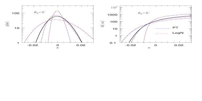
Figure 7: The left panel shows the PDF of the redshift resolved convergence and the right panel shows the associated cumulative bias. The smoothing angular scales considered is $\theta_{0}=5^{\prime}$. Only three tomographic bins are chosen for display to avoid cluttering. Two different approximations are used; the lognormal distribution and the perturbative calculations. The approximations give near identical results. Three different redshift bins are displayed $z_{s}=0.698,1.095,1.493$ (top,middle and bottom curve respectively).

This is one of the most important results in this paper. A few comments are in order, it is possible to integrate the exact expressions of the scaling functions, there is some uncertainty involved in the actual determination of these functions and associated parameters such as $\omega,k_{a},x_{\star}$ from N-body simulations and its unclear how much is there to gain by doing exact calculations that involve approximate picture for the underlying mass distribution; see e.g. Munshi et al. (1999), Valageas et al. (1999) and Colombi et al. (1996) for a detailed description of the effect of the finite volume correction involved in their estimation. Throughout our analysis we have used a top-hat filter for smoothing the convergence field, but the results can easily be extended to compensated or Gaussian filters (Bernardeau & Valageas, 2000). Using Eq.(54) one can derive an approximate expression for the lower order moments which can, in turn, be used to derive order of magnitude relations $S^{\kappa}_{\rm p}=S^{\eta}_{\rm p}/[k^{\rm min}_{(i)}]^{{\rm p}-2}$ for $\rm p>2$. The parameters $S^{\eta}_{\rm p}$ for the underlying density contrast $\delta$ are specified by the choice of a specific hierarchical model. The computation of error bars for these lower order moments can be done using formalism developed in Munshi & Coles (2003).

In Figure (5) we show the PDF of the reduced convergence $\eta$ for smoothing angular scale $\theta_{0}=5^{\prime}$ for the lognormal and hierarchical approximation discussed above, for individual redshift bins as well as for a projected survey.

7.1 The bias associated with convergence maps

To compute the bias associated with the peaks in the smoothed convergence $\kappa$ field we have to first develop an analytic expression for the generating field $\beta_{\kappa}(y_{1},y_{2})$ for the convergence field $\kappa(\theta_{0})$. We will avoid displaying the smoothing angular scale $\theta_{0}$ for brevity. Throughout the statistics are for smoothed convergence fields. For that we will use the usual definition for the two-point cumulant correlator $C_{pq}$ for the convergence field (for a complete treatment see Munshi & Coles, 1999b):

$$C^{(ij)}_{pq}={\langle\kappa_{(i)}({\hat{\Omega}}_{1})^{p}\kappa_{(j)}({\hat{\Omega}}_{2})^{q}\rangle_{c}/[{\bar{\xi}_{2}^{(i)}}]^{p-1}[{\bar{\xi}_{2}^{(j)}}]^{q-1}\xi^{(ij)}_{12}}.$$ (55)

We will show that, like its density field counterpart the two-point generating function for the convergence field $\kappa$ can be expressed (under certain simplifying assumptions) as a product of two one-point generating functions $\beta(y)$ which can then be directly related to the bias associated with “hot-spots”in the convergence field.

$$\beta^{(ij)}_{\eta}(y_{1},y_{2})=\sum_{p,q}^{\infty}{C^{\eta(ij)}_{pq}\over p!q!}y_{1}^{p}y_{2}^{q}=\sum_{p}^{\infty}{C^{\eta(i1)}_{p1}\over p!}y_{1}^{p}\sum_{q}^{\infty}{C^{\eta(j1)}_{q1}\over q!}y_{2}^{q}=\beta^{(i)}_{\eta}(y_{1})\beta^{(j)}_{\eta}(y_{2}).$$ (56)

It is clear that the factorization of generating function depends on the factorization property of the cumulant correlators i.e. $C^{\eta}_{pq}=C^{\eta}_{p1}C^{\eta}_{q1}$. Note that such a factorization is possible when the correlation of two patches in the directions ${\hat{\Omega}}_{1}$ and ${\hat{\Omega}}_{2}$ ${[\xi^{(ij)\kappa}_{12}]}$ is smaller compared to the variance ${[\bar{\xi}^{(ij)}]}$ for the smoothed patches We will now use the integral expression for cumulant correlators (Munshi & Coles 1999a) to express the generating function which in turn uses the hierarchical ansatz and the far field approximation as explained above

$$\beta^{(ij)}_{\kappa}(y_{1},y_{2})=\sum_{p,q}^{\infty}{C^{\eta(ij)}_{pq}\over p!q!}{1\over[\bar{\xi}_{2}^{(i)}]^{p-1}}{1\over[\bar{\xi}_{2}^{(j)}]^{q-1}}{1\over\xi^{12}_{ij}}\int_{0}^{r_{s}}dr{\omega_{(i)}^{p}(r)\omega_{(j)}^{q}(r)\over d_{A}(r)^{2(p+q-1)}}[{\cal J}_{\theta_{12}}(r)][{{\cal J}_{\theta_{0}}(r)}]^{p+q-2}y_{1}^{p}y_{2}^{q}.$$ (57)

It is possible to further simplify the above expression by separating the summation over dummy variables $p$ and $q$, which will be useful to establish the factorization property of the two-point generating function for bias $\beta^{(ij)}(y_{1},y_{2})$. We can now decompose the double sum over the two indices into two separate sums over individual indices. Finally, using the definition of the one-point generating function for the cumulant correlators we can write:

$$\beta^{(ij)}_{\kappa}(y_{1},y_{2})={\int_{0}^{r_{s}}}dr\;d_{A}^{2}(r){{{\cal J}_{\theta_{12}}(r)}\over{[\xi^{(ij)\kappa}_{12}]}}{{[\bar{\xi}_{2}^{(i)\kappa}]}\over{{\cal J}_{\theta_{0}}(r)}}{{[\bar{\xi}_{2}^{(j)\kappa}]}\over{{\cal J}_{\theta_{0}}(r)}}\beta^{(i)}_{\eta}\Big{(}{y_{1}\over{[\bar{\xi}_{2}^{(i)\kappa}]}}{\omega_{(i)}(r)\over d^{2}_{A}(r)}{{\cal J}_{\theta_{0}}(r)}\Big{)}\beta^{(j)}_{\eta}\Big{(}{y_{2}\over{[\bar{\xi}_{2}^{(j)\kappa}]}}{\omega_{(j)}(r)\over d^{2}_{A}(r)}{{\cal J}_{\theta_{0}}(r)}\Big{)}.$$

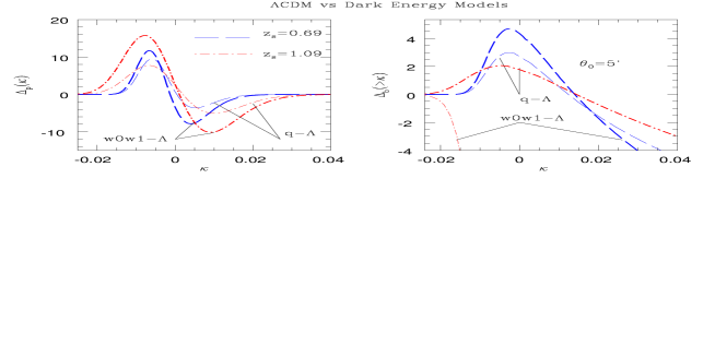
Figure 8: We compare the PDF and cumulative bias associated with tomographic convergence maps for various tomographic bins for two different dark energy models against the $\Lambda$CDM model. The left panel plots the ratio $\Delta_{p}(\kappa)=p(\kappa)-p_{\Lambda{\rm CDM}}(\kappa)$ for a smoothing angular scale of $\theta_{0}=5^{\prime}$. The right panel depicts the ratio $\Delta^{(i)}_{b}(>\kappa)=b^{(i)}(>\kappa)-b^{(i)}_{\Lambda{\rm CDM}}(>\kappa)$ for the cumulative bias. Three different redshift bins are displayed $z_{s}=0.698,1.095$. For a given smoothing angular scale and a fixed redshift, the (thick) curves with higher positive peak heights correspond to the model $w_{0}=-1,w_{1}=1$ and the (thin) ones with lower peak heights correspond to $w_{0}=-0.9$, $w_{1}=0$.

The above expression is quite general within the small approximation and large separation approximations, and is valid for any given specific model for the generating function ${\cal G}_{\delta}(\tau)$. However it is easy to notice that the projection effects as encoded in the line of sight integration do not allow us to write down the two-point generating function $\beta_{\kappa}(y_{1},y_{2})$ simply as a product of two one-point generating functions $\beta_{\eta}(y)$ as was the case for the density field $1+\delta$.

$$\beta_{\kappa}^{(ij)}(y_{1},y_{2})={\int_{0}^{r_{s}}}\;dr\;{d_{A}(r)\over[\kappa^{min}_{(i)}]}{d_{A}(r)\over[\kappa^{min}_{(j)}]}{{{\cal J}_{\theta_{12}}(r)}\over{[\xi^{(ij)\kappa}_{12}]}}{{[\bar{\xi}^{(ij)}]}^{2}\over{{\cal J}_{\theta_{0}}(r)}^{2}}\beta^{(i)}_{\eta}\Big{(}{y_{1}\over{[\bar{\xi}_{2}^{(i)\kappa}]}}{\omega_{(i)}(r)\over d^{2}_{A}(r)}{{{\cal J}_{\theta_{0}}(r)}\over|{\kappa^{\rm min}_{(i)}}|}\Big{)}\beta^{(j)}_{\eta}\Big{(}{y_{2}\over{[\bar{\xi}_{2}^{(j)\kappa}]}}{\omega_{(j)}(r)\over d^{2}_{A}(r)}{{{\cal J}_{\theta_{0}}(r)}\over|{\kappa^{\rm min}_{(i)}}|}\Big{)}.$$ (58)

We use the follwoing equation in assocition with Eq.(53) to simplify the above expression:

$${[\xi^{(ij)\kappa}_{12}]}\approx{1\over 2}r_{s}{\omega_{(i)}(r_{c})\over d_{A}(r_{c})}{\omega_{(j)}(r_{c})\over d_{A}(r_{c})}\Big{[}\int{d^{2}{\bf l}\over(2\pi)^{2}}{\rm P_{\delta}(k)}W_{\rm TH}^{2}(l\theta_{0})\exp[il\cdot\theta_{12}]\Big{]}.$$ (59)

Use of these approximations gives us the leading order contributions to these integrals and we can check that to this order we recover the factorization property of the generating function i.e. $\beta^{(ij)}_{\eta}(y_{1},y_{2})=\beta^{(i)}_{\eta}(y_{1})\beta^{(j)}_{\eta}(y_{2})=\beta^{(i)}_{1+\delta}(y_{1})\beta^{(j)}_{1+\delta}(y_{2})$. So it is clear that at this level of approximation, due to the factorization property of the cumulant correlators, the bias function $b_{\eta}(x)$ associated with the peaks in the convergence field $\kappa$, beyond certain threshold, possesses a similar factorization property too as its density field counterpart. Earlier studies have established such a correspondence between convergence field and density field in the case of one-point probability distribution function $p(\delta)$ (Munshi & Jain 1999b),

$$b_{\eta}^{(i)}(x_{1})h_{\eta}^{(i)}(x_{1})b_{\eta}^{(i)}(x_{2})h_{\eta}^{(j)}(x_{2})=b^{(i)}_{1+\delta}(x_{1})h^{(i)}_{1+\delta}(x_{1})b^{(j)}_{1+\delta}(x_{2})h^{(j)}_{1+\delta}(x_{2}),$$ (60)

where we have used the following relation between $\beta_{\eta}(y)$ and $b_{\eta}(x)$. For all practical purpose we found that the differential bias as defined above is more difficult to measure from numerical simulations as compared to its integral counterpart where we concentrate on the bias associated with peaks above certain threshold. The cumulative bias $b_{\eta}(>x)$ can also be defined in an analogus manner:

$$b_{\eta}(x)h_{\eta}(x)=-{1\over 2\pi i}\int_{-i\infty}^{i\infty}dy\tau(y)\exp(xy);\quad b_{\eta}(>x)h_{\eta}(>x)=-{1\over 2\pi i}\int_{-i\infty}^{i\infty}dy{\tau(y)\over y}\exp(xy).$$ (61)

It is important to notice that, although the bias $b(x)$ associated with the convergence field $\kappa$ and the underlying density field are identical, the variance associated with the density field is very high, while projection effects substantially reduce the variance in the convergence field. This indicates that we have to use the integral definition of bias to recover it from its generating function; see Eq.(61). Now writing down the full two point probability distribution function for two correlated spots in terms of the convergence field $\kappa(\theta_{0})$ and its reduced version $\eta$:

$$\quad\quad\quad\quad\quad\quad\quad\quad\quad\quad\quad\quad\quad\quad\quad\quad p^{(ij)}(\kappa_{1},\kappa_{2})d\kappa_{1}d\kappa_{2}=p^{(i)}(\kappa_{1})p^{(j)}(\kappa_{2})(1+b^{(i)}(\kappa_{1})\xi^{(ij)}_{12}b^{(j)}(\kappa_{2}))d\kappa_{1}d\kappa_{2},$$ (62)

$$\quad\quad\quad\quad\quad\quad p_{\eta}(\eta_{1},\eta_{2})d\eta_{1}d\eta_{2}=p^{(i)}_{\eta}(\eta_{1})p^{(j)}_{\eta}(\eta_{2})(1+b^{(i)}_{\eta}(\eta_{1})\xi^{\eta}_{12}b^{(j)}_{\eta}(\eta_{2}))d\eta_{1}d\eta_{2}.$$ (63)

Using Eq.(54) that $p^{(i)}(\kappa)={p_{\eta}(\eta)/{|\kappa^{(i)}_{\rm min}}|}$ we also notice that $\xi^{(ij)}_{12}={\xi^{\eta}_{12}/{[\kappa^{(i)}_{\rm min}]}{[\kappa^{(j)}_{\rm min}]}}$, from which we can now write:

$$b_{(i)}(\kappa)={b^{(i)}_{\eta}(\eta)/|{\kappa^{(i)}_{\rm min}}|}.$$ (64)

Together with Eq.(54), Eq.(64) can be used to construct analytical estimates of pdf and bias about individual bins. In addition these results are applicable to the modelling of joint PDFs involving two separate redshift bins.

Figure (6) shows the bias associated with the reduced convergence for individual bins as well as for the entire survey. The smoothing angular scale is $\theta_{0}=5^{\prime}$. In Figure (7) shows the PDF and bias associated with the convergence $\kappa$. In Figure (8) we plot the difference in PDF between various cosmological scenarios.

8 Effect of Noise on one- and two-point PDF

The PDF we have considered so far are free from noise. In this section we will present the results of estimates of error relating to the PDFs, those at the level of one-point and two-point PDFs. These results will generalise the ones found by Munshi & Coles (2003) for lower order moments and later by Valageas, Munshi & Barber (2005). Inclusion of noise can be incorporated through a convolution. We will assume the noise to be Gaussian and uncorrelated with the signal. However the variance of the noise will depend on the surface density of galaxies in individual bins. With these simplifying assumption, for the i-th tomographic bin we can write:

$$p^{(i)}_{n}(\kappa)=\int_{-\infty}^{\infty}\;p^{(i)}(\kappa-n)\;p^{(i)}_{G}(n)\;dn.$$ (65)

Here $p^{(i)}_{G}(n)$ is the noise PDF assumed Gaussian, and $p^{(i)}_{n}(\kappa)$ is the convergence PDF in the presence of noise (the subscript $G$ denotes Gaussian). We take $\sigma^{2}_{\kappa}=\sigma^{2}_{\epsilon}/(2n_{g}\pi\theta_{0}^{2})$. Here $\sigma_{\epsilon}$ is intrinsic ellipticity distribution of galaxies and $n_{g}$ is the number denisty of galaxies and $\theta_{0}$ is the smoothing angular scale. The two-point PDF can also be modified to include the effect of noise in a similar manner. The equivalent expression for 2PDF can be written as:

$$p^{(ij)}_{n}(\kappa_{1},\kappa_{2})=p^{(i)}_{n}(\kappa_{1})p^{(j)}_{n}(\kappa_{2})(1+b^{(i)}_{n}(\kappa_{1})\xi^{ij}_{12}b^{(j)}_{n}(\kappa_{2})),$$ (66)

Which is obtained by convolving the noise PDF with the 2PDF:

$$p^{(ij)}_{n}(\kappa_{1},\kappa_{2})=\int_{-\infty}^{\infty}\;p^{(ij)}(\kappa_{1}-n_{1},\kappa_{2}-n_{2})\;p^{(i)}_{G}(n_{1})\;p^{(j)}_{G}(n_{2})\;dn_{1}\;dn_{2}.$$ (67)

Comparing Eq.(66) and Eq.(67) we can write the expression for the noisy bias $b_{n}(\kappa)$ as:

$$b^{(i)}_{n}(\kappa)=\int_{-\infty}^{\infty}p^{(i)}(\kappa-n)b^{(i)}(\kappa-n)p^{(i)}_{G}(n)dn\;/\;\int_{-\infty}^{\infty}p^{(i)}(\kappa-n)p^{(i)}_{G}(n)\;dn.$$ (68)

Notice that depending on redshift distribution of sources, the noise maps $n^{(i)}$ and $n^{(j)}$ can be different for two tomographic bins. We also assumed that noise in different bins are statistically independent. The cumulative bias for the i-th tomographic bin that include noise $b^{(i)}_{n}(>\kappa)$ can be expressed in terms of $p^{(i)}_{n}(\kappa)$ $b^{(i)}_{n}(\kappa)$ just as its noise-free counterpart:

$$b^{(i)}_{n}(>\kappa)=\int_{\kappa}^{\infty}p^{(i)}_{n}(\kappa)b^{(i)}_{n}(\kappa)dk/\int_{\kappa}^{\infty}p^{(i)}_{n}(\kappa)dk.$$ (69)

Errors associated with binned tomographic noisy PDF can be analysed using following quantites:

$${\rm N}=n_{g}\pi\theta_{0}^{2}=314\left({n_{g}\over 100\;{\rm arcmin}^{-2}}\right)\left(\theta_{0}\over 1\;{\rm arcmin}\right)^{2}$$ (70)

Here $n_{g}$ is the number density of galaxies, $\theta_{s}$ is the smoothing angular scale in arc-minutes for a given survey strategy. For a given survey we denote the area covered by $A$ and introduce a parameter $N_{c}$ which will be used in expressing the signal-to-noise estimates of the PDF $p(\kappa)$. We define the following variable that will be useful in qunatifying scatter in a noisy PDF:

$${\rm N}_{c}={A\over(2\theta_{0})^{2}}=2.7\times 10^{4}\left({A\over 300\;{\rm degree}^{2}}\right)\left({\theta_{0}\over 1\;{\rm arcmin}}\right)^{-2}.$$ (71)

Finally the scatter $\sigma(p(\kappa))$ in the measured convergence power sepctra $p(\kappa)$ can be expressed as (Valageas, Munshi & Barber, 2005):

$${\sigma(p^{(i)}_{n}(\kappa))\over p^{(i)}_{n}(\kappa)}=\left[{1\over{\rm N}_{c}}\left({1\over 2p_{n}^{(i)}(\kappa)\Delta}-1\right)\right]^{1/2}$$ (72)

These expression can be modified and used to compute the scatter in individual redshift bins by simply changing $\bar{n}_{g}$ to surface density of individual bins $\bar{n}_{g}^{(i)}$ and $p(\kappa)$ to $p^{(i)}(\kappa)$. The source density for individual bins for a given survey can be computed using $\bar{n}^{(i)}=\int_{z_{i}}^{z_{i+1}}p_{s}(z)dz$. The bin width $\Delta$ is left as a free parameter. In Figure (9) we have plotted the scatter $\sigma(p^{(i)}_{n}(\kappa)$ as a function of intrinsic ellipticity distribution and bin width for a smoothing angular scale of $\theta_{0}=5^{\prime}$ and redshift $z_{s}=0.698$. The results for the difference in noisy PDFs are plotted in Figure (10).

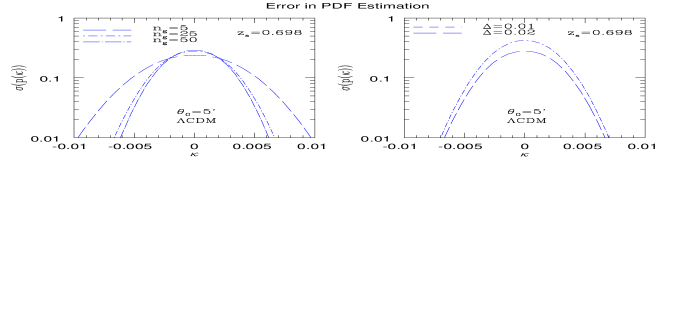
Figure 9: The sacatter in estimation of binned PDF for a given intrinsic ellipticity distribution and sky coverage is displayed. We assume an all-sky coverage. The effect of intrinsic ellipticity distribution is displayed in the left panel. The right panel depicts the effect of binning. The angular scale in each case is $\theta_{0}=5^{\prime}$ and the redshift is $z_{s}=0.698$. The expression for $\sigma(p(\kappa))$ is given in Eq.(72). For the left panel we consider $\Delta=0.02$ and for the right panel $n_{g}=25$. A background $\Lambda$CDM cosmology is accumed for these calculations.

9 Conclusions

Previous tomographic studies of weak lensing have typically worked with the lower order cumulants; we have generalized here these results to the case of the entire one- and two-point PDF, which contain information about the cumulants to an arbitrary order. The construction was performed using a generating function formalism based on hierarchical ansatz and a lognormal model. Our analysis generalizes previously obtained results derived for projected or 2D surveys. Though we have considered a top-hat filer convergence maps due to their simplicity, similar results can be obtained for related statistics such as the shear components or aperture mass $M_{ap}$ (Bernardeau & Valageas, 2000).

The PDFs for the individual bins are constructed by generalization of the previously introduced global variable $\kappa^{\rm min}$, for individual bins i.e.$\kappa^{\rm min}$, that was used in the context of 2D projected maps. Next, using $\kappa_{(i)}^{\rm min}$, reduced variable $\eta^{(i)}$ is defined for each individual bins whose statistics can directly be linked to that of underlying density contrast $\delta$. The convergence in individual bins can then be mapped to unique values of $\eta=1+\delta$ for a given smoothing angular scales $\theta_{0}$.

For modelling the statistics of underlying density contrast $\delta$ we have assumed two completely different model: the hierarchical ansatz along with its perturbative counterpart as well as the lognormal distribution. Both these approximations have been used successfully in various cosmological contexts. There are a wide class of models that are available under the general category of hierarchical ansatz. The main motivation behind our choice of a specific hierarchy is simplicity. In recent years more sophisticated models of hierarchical clustering have been proposed which rely more on inputs from numerical simulations. The generic results we have derived here indeed can be improved using such modelling though the fundamental characteristics will remain unchanged.

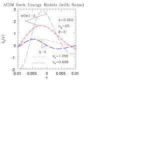
Figure 10: The difference of noisy $\Lambda$CDM PDF and dark energy models $\Delta_{p}(\kappa)=p(\kappa)-p_{\Lambda\rm CDM}(\kappa)$ is plotted as a function of $\kappa$. The smoothing angular scale, bin size and galaxy number density is as depicted. The scatter in estimation is smaller compared to the difference in the PDFs considered. The comsological parameters considered are the same as the ones in Figure-(8). The two survey configurations that we have considered both produces near identical results.

In our treatment we find, in agreement with Munshi & Wang (2003), the dynamical and geometrical contribution can be treated separately. The geometrical effects are completely encoded in a parameter $\kappa^{min}$. The reduced convergence as defined is independent of the background geometry of the universe and essentially probe the evolution of gravitational clustering. We showed that a set of $\kappa^{\rm min}_{(i)}$ defined for a given set of redshift slices are adequate to characterize not only individual PDFs for each bin but it is also sufficient to study the joint two-point PDF among two different bins. The PDF of the reduced convergence $\eta^{(i)}$ for individual bins or joint PDFs for a pair of bins generalizes the earlier studies where the projected or 2D maps were considered in a straight forward manner.

We also note that the construction of convergence maps is difficult compared to the direct evaluation of non-Gaussian statistics from shear maps. On the other hand convergence statistics can directly be modelled at arbitrary order whereas for shear field the computation is done mostly order by order manner. An independent analysis of convergence maps constructed from shear maps should therefore be useful in constraining various errors which might get introduced during various stages of data reduction.

In our analysis we have ignored the noise from intrinsic ellipticity distribution of galaxies as well as from shot noise resulting from finite number of galaxies that are used to trace the underlying mass distribution. These issues have been dealt with in great detail in Munshi & Coles (2003); Valageas, Barber & Munshi (2004). Dividing the source population into bins reduced the number-density of sources. This in turn will increase the level of noise or the scatter in the estimator. In our analysis we have considered two different survey configurations, i.e. LSST and DES and found that for our choice of tomographic bins the one- and two-point PDFs are very similar in nature.

The lognormal distribution has already been used to model the statistics of weak lensing observables (Munshi, 2000; Taruya et al., 2002) and the clustering of Lyman alpha absorption systems e.g. (Bi & Davidson, 1997). One-to-one mapping of initial density fields to evolved density fields using maps that are consistent with lognormal distribution function was not found to be very successful and the success of a lognormal distribution function in reproducing the statistics of gravitational clustering still remains somewhat unclear.

Tomographic weak lensing surveys can be cross-correlated with external data sets including frequency cleaned maps of secondaries from ongoing CMB surveys; e.g. the thermal Sunyaev-Zeldovic (tSZ) maps or $y$-maps that will be available from CMB surveys such as Planck. The cross-correlation with tomographic information can help to understand the evolution of cosmological pressure fluctuations responsible for tSZ effect with redshift. The formalism presented here is perfectly suitable for such analysis. Detailed results of such analysis will be presented elsewhere. In addition to the weak lensing surveys the Supernova pencil beam surveys might also benefit for the results presented here.

To summarize, we have extended results derived in three different previous papers (Munshi & Coles, 2003; Valageas, Munshi & Barber, 2005; Valageas, Barber & Munshi, 2004) to take into account tomographic bins within which the photometric redshift are available. The results obtained previously for one-point PDF are now extended to two-point PDF. These results can provide an alternative to usual Fisher-matrix analysis that is employed to optimize survey strategies. We have concentrated mainly on analytical results in this paper. The numerical results regarding optimization of survey strategy using these results will be considered elsewhere.

10 Acknowledgements

DM and PC acknowledges support from STFC standard grant ST/G002231/1 at School of Physics and Astronomy at Cardiff University where this work was completed. We would like to thank Alan Heavens, Patrick Valageas, Ludo van Waerbeke and Sanaz Vafei for many useful discussions. The numerical results were obtained using a modified version of a code made available to us for computing the PDF and bias by Francis Bernardeau.

References

- Amendola & Tsujikawa (2010) Amendola L.,Tsujikawa S., Dark Energy: Theory and Observations, Cambridge University Press ISBN-10: 0521516005
- Beacon, Refregier & Ellis (2000) Beacon D.J., Refregier A., Ellis R.S., 2000, MNRAS, 318, 625
- Bernardeau et al (2002) Bernardeau F., Colombi S., Gaztanaga E., Scoccimarro R., 2002, Phys.Rept.,367, 1
- Bernardeau & Schaeffer (1992) Bernardeau F., Schaeffer R., 1992, A&A, 255, 1
- Bernardeau (1992) Bernardeau F. 1992, ApJ, 392, 1
- Bernardeau (1994) Bernardeau F. 1994, A&A, 291, 697
- Bernardeau & Kofman (1995) Bernardeau F., Kofman L. 1995, ApJ, 443, 479
- Bernardeau & Valageas (2000) Bernardeau F., Valageas P., 2000, A&A, 364, 1
- Bi & Davidson (1997) Bi H.G., Davidson A.F. 1997, ApJ, 479, 523
- Bouchet et al (1993) Bouchet, F., Strauss, M. A., Davis, M., Fisher, K. B., Yahil, A., Huchra, J. P. 1993, ApJ, 417, 36
- Castro et al (2005) Castro P.G., Heavens A.F., Kitching T.D., 2005, Phys.Rev. D72, 023516
- Coles (1988) Coles P., 1988, MNRAS, 234, 509
- Coles & Jones (1991) Coles P., Jones B. 1991, MNRAS, 248,1
- Colombi (1994) Colombi S., 1994, ApJ, 435, L536
- Colombi et al. (1997) Colombi S., Bernardeau F., Bouchet F. R., Hernquist L. 1997, MNRAS, 287, 241
- Cooray & Seth (2002) Cooray A., Seth R., 2002, Phys. Rep. 372, 1
- Fry (1984) Fry J.N., 1984, ApJ, 279, 499
- Hamilton (1985) Hamilton, A. J. S. 1985, ApJ, 292, L35
- Hamilton et al. (1985) Hamilton, A. J. S., Kumar P., Lu E., Matthew A., 1991, ApJ, 374, L1.
- Heavens (2003) Heavens A.F., 2003, MNRAS, 343, 1327
- Heavens, Refregier & Heymans (2000) Heavens A. F., Refregier A., Heymans C.E., 2000, MNRAS, 319, 649
- Heavens, Kitching & Taylor (2006) Heavens A. F., Kitching T. D., Taylor A.N., 2006, MNRAS, 373, 105
- Heavens, Kitching & Verde (2007) Heavens A. F., Kitching T. D., Verde L., 2007, MNRAS, 380, 1029
- Hui (1999) Hui L., ApJ.,1999, 519, L9
- Hu (1999) Hu W., ApJ., 1999, 522, L21
- Jain & Seljak (1997) Jain B., Seljak U., 1997, ApJ, 484, 560
- Jain, Seljak & White (2000) Jain B., Seljak U., White S. Astrophys.J., 2000, 530, 547
- Kaiser (1992) Kaiser N. 1992. ApJ, 388, 272
- Kaiser, Wilson & Luppino (2000) Kaiser N., Wilson G., Luppino G.A., astro-ph/0003338
- Kayo, Taruya, Suto (2001) Kayo I., Taruya A., Suto Y. 2001, ApJ, 561, 22
- Kitching et al. (2008) Kitching T.D., Heavens A. F., Verde L., Serra P., Melchiorri A., PRD. 2008, 77, 103008
- Kofman et al. (1994) Kofman, L., Bertschinger, E., Gelb, J. M., Nusser, A., Dekel, A. 1994, ApJ, 420, 44
- Limber (1954) Limber D.N., 1954, ApJ, 119, 665
- Matarresse et al. (1992) Matarrese S., Lucchin F., Moscardini L., Saez D., 1992, MNRAS, 259, 437
- Munshi et al. (2011) Munshi D., van Waerbeke L., Smidt J., Coles P., arXiv:1103.1876
- Munshi, Sahni, Starobinsky (1994) Munshi D., Sahni V., Starobinsky A., 1994, ApJ, 436, 517
- Munshi & Heavens (2010) Munshi D., Heavens A. 2010, MNRAS, 401, 2406
- Munshi & Jain (2000) Munshi D., Jain B., 2000, MNRAS, 318, 109
- Munshi & Jain (2001) Munshi D., Jain B., 2001, MNRAS, 322, 107
- Munshi et al. (2008) Munshi D., Valageas P., van Waerbeke L., Heavens A., 2008, PhR, 462, 67
- Munshi (2000) Munshi D., 2000, MNRAS, 318, 145
- Munshi et al (1999) Munshi D., Bernardeau F., Melott A.L., Schaeffer R.,1999, MNRAS, 303, 433
- Munshi & Coles (2000) Munshi D., Coles P., 2000, MNRAS, 313, 148
- Munshi & Coles (2002) Munshi D., Coles P., 2002, MNRAS, 329, 797
- Munshi & Coles (2003) Munshi D., Coles P., 2003, MNRAS, 338, 846
- Munshi, Coles & Melott (1999a) Munshi D., Coles P., Melott A.L., 1999a, MNRAS, 307, 387
- Munshi, Coles & Melott (1999b) Munshi D., Coles P., Melott A.L., 1999b, MNRAS, 310, 892
- Munshi, Melott & Coles (1999) Munshi D., Melott A.L., Coles P., 1999, MNRAS, 311, 149
- Valageas & Munshi (2004) Munshi D., Valageas P., 2004, MNRAS, 354, 1165
- Munshi, Valageas & Barber (2004) Munshi D., Valageas P., Barber A. J., 2004, MNRAS, 350, 77
- Munshi & Wang (2003) Munshi D, Wang Y., ApJ., 2003, 583, 566
- Munshi, Heavens & Coles (2011) Munshi D., Heavens A. Coles D., 2011, MNRAS, 411, 2161
- Munshi et al. (2011) Munshi D., Smidt J., Heavens A., Coles P., Cooray A., 2011, MNRAS, 411, 2241
- Munshi et al. (2011b) Munshi D., Smidt J., Joudaki S., Coles P. 2011, MNRAS (submitted)
- Munshi & Padmanabhan (1997) Munshi D., Padmanabhan T. 1997, MNRAS, 290, 193
- Peebles (1980) Peebles P.J.E. 1980, “The Large Scale Structure of the Universe” (Princeton University Press).
- Pen et al. (2003) Pen Ue-Li et al, 2003, ApJ., 592, 664
- Peacock & Dodds (1994) Peacock J.A., & Dodds S.J., 1994, MNRAS, 267, 1020
- Planck Collaboration (2006) Planck Collaboration, 2006, astro-ph/0604069
- Rhodas, Gott & Postman (1994) Rhoads, J.E., Gott J.R.I., Postman M. 1994, ApJ, 421, 1
- Sato et al. (2001) Sato J., Takada M., Jing Y.P., Toshifumi F., 2001,, ApJL, 551,5
- Schaeffer (1984) Schaeffer R., 1984, A&A, 134, L15
- Schamalzing & Buchert (1997) Schamalzing & Buchert 1997, ApJ, 482, L1
- Scoccimarro et al (1998) Scoccimarro R. et al, ApJ., 1998, 496 586
- Semboloni et al (2008) Semboloni et al, 2008, MNRAS, 388, 991
- Szapudi & Szalay (1993) Szapudi I., Szalay A.S., 1993, ApJ, 408, 43
- Szapudi & Szalay (1997) Szapudi I., Szalay A.S., 1997, ApJ, 481, L1
- Takada & Jain (2004) Takada M., Jain B., MNRAS, 2004, 348, 897
- Takada & Jain (2003) Takada M., Jain B., 2003, MNRAS, 344, 857
- Takada & White (2003) Takada M., White M., 2001, ApJ. 601, L1
- Taruya et al. (2002) Taruya, A., Takada, M., Hamana, T., Kayo, I., Futamase, T., 2002, ApJ, 571, 638
- Taruya et al. (2002) Taruya A., Takada M., Hamana T., Futamese T., 2002, ApJ, 571, 638
- Waerbeke et al (2000) van Waerbeke L. et al. 2000, A&A, 358, 30
- Valageas, Munshi & Barber (2005) Valageas P., Munshi D., Barber A. J., 2005, MNRAS, 356, 386
- Valageas, Barber & Munshi (2004) Valageas P., Barber A. J., Munshi D., 2004, MNRAS, 347, 654
- Valageas (2000) Valageas P., 2000, A&A, 356, 771
- Villumsen (1996) Villumsen J.V. 1996, MNRAS, 281, 369
- Wang (2010) Wang Y., Dark Energy, Wiley-VCH; ISBN-10: 9783527409419
- Wang & Ganrnavich (2001) Wang Y., Garnavich P., 2001, ApJ, 552, 445
- Wittman et al (2000) Wittman D. et al. 2000, Nature, 405, 143