Foreground Analysis Using Cross-Correlations of External Templates on the 7-year WMAP data

Abstract

WMAP data when combined with ancillary data on free-free, synchrotron and dust allow an improved understanding of the spectrum of emission from each of these components. Here we examine the sky variation at intermediate and high latitudes using a cross-correlation technique. In particular, we compare the observed emission in several large partitions of the sky plus 33 selected sky regions to three “standard” templates. The regions are selected using a criterion based on the morphology of these template maps.

The synchrotron emission shows evidence of steepening between GHz frequencies and the WMAP bands. There are indications of spectral index variations across the sky but the current data are not precise enough to accurately quantify this from region-to-region.

The emission correlated with the H_α template shows clear evidence of deviation from a free-free spectrum. The emission can be decomposed into a contribution from both free-free and spinning dust in the warm ionised medium of the Galaxy. The derived free-free emissivity corresponds to a mean electron temperature of $\sim 6000$ K, although the value depends critically on the impact of dust absorption on the H_α intensity. The WIM spinning dust emission has a peak emission in intensity in the range 40–50 GHz.

The anomalous microwave emission associated with dust is detected at high significance in most of the 33 fields studied. The anomalous emission correlates well with the Finkbeiner et al. (1999) model 8 predictions (FDS8) at 94 GHz, and is well described globally by a power-law emission model with an effective spectral index between 20 and 60 GHz of $\beta\approx-2.7$. It is clear that attempts to explain the emission by spinning dust models require multiple components, which presumably relates to a complex mix of emission regions along a given line-of-sight. An enhancement of the thermal dust contribution over the FDS8 predictions by a factor $\sim 1.2$ is required with such models. Furthermore, the emissivity varies by a factor of $\sim 50\%$ from cloud to cloud relative to the mean.

The significance of these results for the correction of CMB data for Galactic foreground emission is discussed.

1 Introduction

A major goal of observational cosmology is to determine those parameters that describe the Universe. Observations of the Cosmic Microwave Background (CMB) at frequencies in the range 20 – 200 GHz provide unique data to achieve this by establishing the statistical properties of temperature (and polarisation) measurements. However, an impediment to such studies arises due to foreground emission in our own Galaxy from at least three sources – synchrotron, free-free and thermal dust emission. As CMB studies move to ever higher precision it is essential to determine the properties of these components to similarly high accuracy. Indeed, although the combined foreground level reaches a minimum in this frequency range ($\nu\approx 70$ GHz), it remains the dominant signal over large fractions of the sky. Of particular relevance to this discussion is the fact that each of the foreground components has a spectral index that varies from one line of sight to another so using a single spectral index can lead to significant uncertainties in the corrections required. It is therefore essential to study the nature of the Galactic signal at microwave wavelengths in its own right.

All-sky observations by the Wilkinson Microwave Anisotropy Probe (WMAP, Bennett et al., 2003a) at the 5 frequencies of 23, 33, 41, 61 and 94 GHz can provide the basis for improving our understanding of local foregrounds. By comparing these maps with templates for synchrotron, free-free and dust emission, made at frequencies where the specific emission mechanisms dominate, it is possible to clarify important properties of the emission. Indeed, new insights into the nature of the Galactic diffuse emission have arisen from studies of the WMAP data, including the detection of several unexpected new contributions.

Anomalous dust-correlated emission (Leitch et al., 1997) was originally observed in the COBE-DMR data (Kogut et al., 1996) but was thought to be due to free-free emission. Draine & Lazarian (1998a,b) shifted attention to the dust itself as the source of emission through a mechanism now referred to as “spinning dust”, or dipole emission from very rapidly spinning grains. A reanalysis of the intermediate and high Galactic latitude data taken by COBE-DMR and supplemented by 19 GHz observations (Banday et al., 2003) led to evidence for dust at intermediate Galactic latitudes emitting a spectrum consistent with the the form expected for spinning dust, specifically a hint of a turnover at frequencies below $\sim$ 20 GHz. However, study of the WMAP data has allowed further refinement of our understanding of the emission. Cross-correlation of the K-band data with observations at 15 GHz (de Oliveira-Costa et al., 2004) again indicated a plateau or downturn in foreground emission inconsistent with a free-free or synchrotron origin. Lagache (2003) compared the WMAP data to HI column density measurements,revealing an increase in emission with decreasing density, suggesting that the anomalous emission is connected to small, transient heated grains. In addition, a series of papers (Finkbeiner, 2004; Dobler & Finkbeiner, 2008a, b) have strongly confirmed the presence of anomalous dust emission in the WMAP data, and claim to have found evidence of such a component from the diffuse warm ionised medium (WIM) of the Galaxy. Specifically, the correlation with a H_α template, commonly utilised as a proxy for the free-free emission, is not consistent with the spectrum expected for ionised gas, and a broad bump is seen peaking towards $\sim$ 40 GHz. Subsequently, Dobler, Draine & Finkbeiner (2009) have attempted to constrain specific spinning dust parameters such as the density and typical electric dipole moment of the grains. Recently, Peel (2011) have shown that the K-band dust-correlated component is not strongly affected by the inclusion of a 2.3 GHz synchrotron template, reducing the possibility of a flat-spectrum synchrotron component.

Finally, the so-called WMAP-haze was identified by Finkbeiner (2004) although it was already clearly apparent in the foreground residuals of Bennett et al. (2003b) and subsequently in the SMICA analysis of Patanchon et al. (2005). The initial physical interpretation of the haze was that it was associated with free-free emission from hot gas in excess of $10^{5}$ K, but this was refuted on the basis of the lack of associated X-ray emission. The detection of the haze relies upon the use of standard templates to remove known foreground emission utilising spatially independent spectra over the entire (high-latitude) sky. It has been argued that such a crude approximation to the true behaviour of the foreground emission at microwave frequencies may well lead to unphysical results. Indeed, Gold et al. (2011) find that a spatial variation of spectral index of order 0.25 between 408 MHz and K-band is sufficient to reproduce the haze amplitude. Furthermore, a corresponding polarised signal was found to be absent from the WMAP data. However, the lack of polarised emission can be explained by the entanglement of the Galactic magnetic field towards the Galactic centre, leading to a lower polarisation fraction there as compared to the outer Galaxy. Nevertheless, the microwave haze remains an active area of research, particularly given its possible association with a gamma-ray counterpart observed in the Fermi data (Dobler et al., 2010).

In this paper, we characterise the spatial variation in the foreground emission in terms of the various emission mechanisms noted above by introducing a new partition of the sky into morphologically selected regions. In previous work (Davies et al., 2006, hereafter D06), our approach was to identify regions away from the Galactic plane which were expected to be dominant in one of the three foreground components, free-free, synchrotron or dust and to derive the spectrum for each component. Five regions covering angular scales of $3\deg$ to $20\deg$ were chosen for each component, based on foreground template maps, making 15 in all. Here, we generalise this approach and introduce an algorithm to define a set of 35 regions for further study. The selection is intended to minimise the potential cross-talk between the various physical components and to select regions over which the spectral behaviour is uniform thus supporting the use of a template-based comparison. We use a well-known and understood cross-correlation technique to undertake the analysis.

The paper is organised as follows. Section 2 describes the WMAP data and foreground templates used in this analysis while Section 2.3 defines the regions of interest for investigation. The methodology of the cross-correlation analysis is outlined in Section 3 and the corresponding results are presented in Section 4. Model-dependent spectral fits for each component are considered in Section 5 and overall conclusions given in Section 6. Appendix A discusses in detail issues related to the H_α template used in the analysis, Appendix B defines the detailed method for partitioning the sky, and finally Appendix C tabulates all of the template-fit coefficients for all the regions analysed.

2 Data used in the analysis

2.1 WMAP data

We use the WMAP seven-year data (Jarosik et al., 2011) provided in the HEALPix pixelisation scheme (Górski et al., 2005) with associated resolution $N_{side}$=512 that can be obtained from the Legacy Archive for Microwave Background Data Analysis (LAMBDA) website. The WMAP satellite has 10 so-called differencing assemblies (DAs) distributed over five frequencies from $\sim$23 GHz (K-band) to $\sim$ 94 GHz (W-band), and with frequency-dependent resolutions ranging from approximately $0^{\circ}\!.93$ up to $0^{\circ}\!.23$. The K- and Ka-bands have only one DA each, Q and V band have two each, while W-band has four.

Multiple DAs at each frequency for the Q-, V- and W-bands are combined using simple averaging to generate a single map per frequency band. The data are then smoothed to a common resolution of $3^{\circ}$ (after deconvolving the effective azimuthally symmetric beam response for each map) and degraded to HEALPix $N_{side}$=64. We perform our analysis at this resolution, rather than the more typical $1^{\circ}$ studies, to account for the full covariance properties of the signal (see section 3). We have also identified a problem with using the H_α data at higher resolution, as discussed further in section 2.2 and Appendix A. Finally, we convert the data to brightness (antenna) temperature units from thermodynamic temperature since this is more appropriate for studying the spectral dependences of foregrounds.

2.2 Foreground templates

Each of the templates used here has been discussed at length in many prior studies. Thus we provide only a brief review and refer the reader to D06 and references therein.

Synchrotron Template: The synchrotron emission arises mainly due to the acceleration of relativistic cosmic ray electrons in the Galactic magnetic field. Thus, the brightness temperature of the synchrotron spectrum depends on the energy spectrum of the cosmic ray electrons and the strength of the magnetic field. For an electron population with energy distribution $N(E)$ given by a power law, $N(E)dE\propto E^{-\delta}dE$ , the brightness temperature of the ensemble synchrotron spectrum is also a power law given by, $T(\nu)\propto\nu^{\beta_{s}}$, where $\beta_{s}$ is related to spectral index of the energy spectrum $\delta$ by the relation $\beta_{s}=(\delta+3)/2$. At very low frequency ($<$ 1 GHz), the observed sky signal is dominated by the synchrotron emission from our Galaxy, and is least contaminated by free-free emission, at least away from the Galactic plane. The spectral behaviour changes with frequency as a result of the details of cosmic-ray electron propagation. Indeed, the mean spectral index changes typically from $\beta_{s}=-2.55$ to $-2.8$ at 38 and 800 MHz respectively (Lawson et al., 1987). Moreover, $\beta_{s}$ varies across the sky and a range of values from $-2.3$ to $-3.0$ has been determined by Reich & Reich (1988) between 408 and 1420 MHz data. The 408 MHz radio continuum survey of Haslam et al. (1982) provides a full sky template for synchrotron studies at an angular resolution close to $1^{\circ}$. For our purpose, we use the version of the data provided by the LAMBDA site.

Free-Free Template: Free-free emission arises in regions of ionised hydrogen and is produced by free electrons scattering from ions without capture. The intensity spectrum of the free-free emission depends on the electron temperature and emission measure (EM) which is related to the number density of electrons ($n_{e}$) along a given line of sight as EM=$\int n_{e}^{2}dl$. The optical H_α recombination line results from the capture of free electrons by a proton nucleus and is therefore also related to the EM. A high resolution full sky map of H_α emission can then be used as a good tracer of the free-free continuum emission at radio wavelengths. There is a well-defined relationship between the H_α intensity and radio-continuum brightness temperature with a strong dependence on frequency and modest dependence on electron temperature $T_{e}$. Dickinson, Davies & Davis (2003, hereafter DDD) generated a full-sky H_α map as a composite of WHAM data in the northern sky (Reynolds et al., 1998; Haffner, 1999) and the SHASSA survey (Gaustad et al., 2001) in the south. We refer the reader to their paper for more complete details.

A significant uncertainty when using the H_α template is the absorption of H_α by foreground dust. The absorption can be estimated by using the dust column density maps of Schlegel, Finkbeiner & Davis (1998, hereafter SFD), and the parameter $f_{d}$ corresponding to the fraction of dust in front of the H_α that causes the absorption. DDD showed that for Galactic longitudes in the range $l$ = 30^∘ – 60^∘ and latitudes $\mid\,b\,\mid$ = 5^∘ – 15^∘, $f_{d}\sim$ 0.3. However, for local high latitude regions such as Orion and the Gum nebula there is little or no absorption by dust. This was also the interpretation favoured for high latitude H_α template fits to the COBE-DMR data in Banday et al. (2003). We adopt a default value $f_{d}\ =\ 0$ in this paper, but consider the impact of varying the absorption parameter on our results. We note that there is an effective degeneracy between $f_{d}$ and electron temperature $T_{e}$ for the interpretation of the fits between the WMAP data and the H_α template, and that the majority of such analyses assume that the dust is coextensive with the H_α emission, i.e. $f_{d}\sim$ 0.5.

An alternative H_α template has been assembled by Finkbeiner (2003) using additional data that provides higher angular resolution on limited areas of the sky. We have examined and compared these two templates in detail and discuss the comparison in Appendix A. In summary, we find that there are inconsistencies in the template fit results obtained with the two templates that are resolved only by smoothing the data to a resolution lower than $1^{\circ}$. For our main results we choose a resolution of $3^{\circ}$. Such differences were already visible in the results of D06. These may be connected with a subtle interplay between artefacts in the H_α templates and the template fitting method we utilise that leads to unstable estimates of the amplitude of the correlated emission at a given frequency. We use exclusively the DDD template fits in this work since the template was explicitly constructed to have uniform resolution.

Dust Template: Thermal dust emission is the dominant foreground at frequencies of 100 – 1000 GHz. Its emissivity is generally modelled by a modified blackbody spectrum, $I(\nu)\propto\ \nu^{\alpha_{d}}\,B_{\nu}(T_{d})$, where $\alpha_{d}$ is the emissivity index and $B_{\nu}(T_{d})$ is the blackbody emissivity at a dust temperature $T_{d}$. Finkbeiner, Davis & Schlegel (1999, hereafter FDS) predicted the thermal dust contribution at microwave frequencies from a series of models based on the COBE-DIRBE 100 and 240 $\mu m$ maps tied to COBE-FIRAS spectral data. The preferred model 8 (FDS8) has an effective power-law spectral index in antenna temperature of $\beta_{d}\approx+1.55$ over the WMAP frequencies. We use the FDS8 predicted emission at 94 GHz as our reference template for dust emission, and demonstrate that it also traces the anomalous component that predominates in the 10–100 GHz frequency range. Fits of the template to the WMAP data will help to constrain the spectral dependence of the dust-correlated foregrounds, and allow comparison to spinning dust models. Nevertheless, we note that an alternative for the spinning dust component may ultimately be required. Indeed, Finkbeiner (2004) proposed that an anomalous dust template could be better constructed using FDS8$\times{\rm T_{d}}^{2}$, however D06 find little evidence for this. More recently, Ysard, Miville-Deschênes & Verstraete (2010) have found improved correlation between the AME and the 12 $\mu$m brightness divided by the intensity of the interstellar radiation field in 27 fields of area 5^∘ squared. However, such a template is not available at present for the full-sky given the difficulty in adequately cleaning the 12 $\mu$m data from residual zodiacal emission.

2.3 Masks for Global fits

In order to examine the largest scale properties of the foregrounds, we have performed fits over large sky areas defined by two basic masks (EBV and KQ85) and the intersection of the former with the Northern and Southern hemispheres defined in various reference frames (Galactic and ecliptic). We have also tested the sensitivity of the Northern hemisphere fits to the inclusion or otherwise of the North Polar Spur (NPS) region defined with reference to the 408 MHz radio survey. A representative subset of the effective masks are shown in Fig. 1. We collectively refer to analyses made using these masks as global fits.

The KQ85 mask was developed by the WMAP team for the primary purpose of cosmological analysis. Since we are interested in investigating the properties of the foreground sky, our default EBV base mask is not as conservative as the KQ85 mask that may exclude some areas of interest in our analysis.

We define the EBV mask by rejecting that fraction of the sky for which the dust absorption in the H_α survey is unreliable. In practice, this corresponds to the sky area where the absorption, as related to the dust optical depth maps from SFD and the conversion factors in DDD, exceeds 1 magnitude. This analysis is carried out at 3 degree FWHM resolution, then the extinction map is downgraded to a HEALPix pixel resolution $N_{side}=64$. This is then merged with the downgraded WMAP7 processing and point source masks in which any partially filled low resolution pixels are explicitly masked. Some additional pixels are also excluded corresponding to regions around the LMC, SMC and high-latitude clusters where some signal appears to leak outside the mask when applied to the WMAP7 K-band data smoothed to 3 degrees FWHM.

For reference, we have included some fits based on the KQ85 mask. The Galactic plane part of the mask was smoothed to 3 degree resolution, then downgraded to $N_{side}=64$ and those pixels with a value less than 0.95 were then rejected (set to 0) and those above were accepted (set to 1). This was subsequently merged with the point source mask as used to create the EBV mask.

Finally, the NPS may impact the synchrotron spectral indices determined in the Northern hemisphere. To test this, we apply a crude masking of the NPS. This is based on the observation that the 408 MHz map smoothed to 3 degrees resolution and divided by the cosecant of the Galactic latitude (an approximation to remove the path-length dependence of the emission within the Galaxy), shows an obvious enhancement towards the NPS compared to the rest of the sky. Thresholds are then applied to the map to eliminate data until there are no pixels in the North with values exceeding the maximum in the South (for Galactic latitudes less than $-5$ degrees). The resulting mask is certainly visually compelling as seen in Fig. 1.

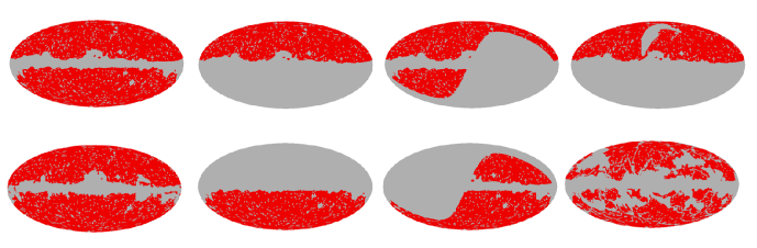
Figure 1: A representative set of global masks used on this analysis. Masked areas are in blue. From left to right and from top to bottom : (1) EBV mask with point source mask included, (2) Galactic North Mask, (3) Ecliptic North Mask, (4) Galactic North Mask with North Polar Spur(NPS) removed (5) KQ85 mask with point source mask included, (6) Galactic South Mask (7) Ecliptic South Mask, (8) For reference, this shows the effective mask that would result if all of the 33 regions were combined and the EBV mask subsequently imposed. The individual regions are shown in Fig. 2. Note that this mask has not been used for analysis.

2.4 Regions Definition

In this paper, we define a new set of regions generalising the approach from Davies et al. (2006). In this previous analysis, regions were selected on the basis that one of the three foregrounds (free-free, dust or synchrotron emission as traced by standard templates) was dominant in each region. We extend this morphological definition in Appendix B, the result of which is the set of 35 candidate regions seen in Fig. 2. For analysis purposes, the regional mask is combined with the EBV mask, and this renders two candidate regions sufficiently small that we elect to omit them, leaving 33 regions for further study. These two regions can be seen in the figure but are not enumerated. Note that region 3 contains the NPS, but we do not attempt to suppress its impact by application of the NPS mask. In addition, our analysis is largely insensitive to the WMAP haze given that the sky areas where this is most prominent are not selected by our region definition scheme. This should be of little surprise given that the definition is based on the 408 MHz data in part, and haze emission is not seen therein. Various properties of the regions are specified in Table 7.

We stress that we do not claim any absolute optimality of these regions for analysis. Indeed, they are by no means unique, and many alternate methods for regional definition are plausible. In fact, we recognise that, although we have applied a cosecant flattening to the data to allow their definition, such a flattening has not been applied in analysis and the fits may still be sensitive to the largest-scale Galactic emission as a function of latitude. Given the morphology of our regions, and the large range of latitudes that some cover (particularly towards the North Galactic pole) this could be a potential consequence of our approach. However, if there were a strong effect, it would be seen by comparing intermediate latitudes with high latitudes.

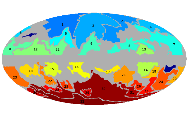
Figure 2: The set of regions defined in Appendix B. 35 candidate regions have been identified, but two (here in dark blue and not enumerated) were considered to be too small after the EBV mask has also been applied for analysis purposes. 33 regions are analysed in this paper.

3 Methods

The aim of this work is to cross-correlate datasets at different wavelengths in regions of the sky defined by the morphology of the templates described in § 2. The cross–correlation (C–C) method used here is a least–squares fit of one map to one or more templates. We perform the analysis at a resolution of 3^∘ FWHM on sky maps degraded to a HEALPix pixel resolution specified by $N_{side}=64$ rather than the more typical $1^{\circ}$ analysis seen, for example, in D06. This allows us to take account of the full covariance properties of the signal, and also provides a solution to some issues related to the the H_α data at higher resolution, as discussed further in Appendix A. In this way, we can include information about the CMB through its signal covariance rather than having to correct for it.

It should be noted that in the high signal-to-noise regime probed by WMAP7 data, the CMB covariance dominates the error budget in the fits. A different approach, as advocated for example by Finkbeiner (2004); Dobler & Finkbeiner (2008a, b), removes an estimate of the CMB signal from the data before cross-correlation. Such an internal linear combination (ILC) map typically corresponds to a linear combination of the data at the 5 WMAP frequencies. However, in principle this also correlates the fits between frequencies due to the common noise properties of the ILC map. More seriously, since the ILC contains foreground residuals, the subtraction changes the relative levels of foreground emissions at each frequency depending on the spectral characteristics of a given component. An approach to rectify this has been specified in Dobler & Finkbeiner (2008a). However, we prefer to retain the approach from D06 in this analysis.

3.1 Cross - Correlation Analysis

The cross–correlation measure, $\alpha$, between a data vector, ${\bf d}$ and a template vector ${\bf t}$ can be measured by minimising:

$$\chi^{2}=({\bf d}-\alpha{\bf t})^{T}\cdot{\bf M}^{-1}_{SN}\cdot({\bf d}-\alpha{\bf t})={\bf\tilde{d}}^{T}\cdot{\bf M}^{-1}_{SN}\cdot{\bf\tilde{d}}$$ (1)

where ${\bf M}_{SN}$ is the covariance matrix including both signal and noise for the template–corrected data vector ${\bf\tilde{d}}\equiv{\bf d}-\alpha{\bf t}$. Solving for $\alpha$ then becomes:

$$\alpha=\frac{{\bf t}^{T}\cdot{\bf M}^{-1}_{SN}\cdot{\bf d}}{{\bf t}^{T}\cdot{\bf M}^{-1}_{SN}\cdot{\bf t}}$$ (2)

To compare multiple template components ${\mathbf{t}}_{j}$, e.g., different foregrounds, to a given dataset, the problem becomes a matrix equation. In the case where we have $N$ different foreground components, we end up with the simple system of linear equations ${\bf Ax}={\bf b}$,where

$$A_{kj}=\mathbf{t}^{T}_{k}\cdot\mathbf{M}_{\textrm{SN}}^{-1}\cdot\mathbf{t}_{j},$$

$$b_{k}=\mathbf{t}^{T}_{k}\cdot\mathbf{M}_{\textrm{SN}}^{-1}\cdot\mathbf{d},$$

$$x_{k}=\alpha_{k}.$$ (3)

When only one template is present, this reduces to equation 2 above.

The signal covariance is that for theoretical CMB anisotropies, $M^{S}_{ij}=\frac{1}{4\pi}\sum^{\infty}_{\ell=0}(2\ell+1)C_{\ell}B^{2}_{\ell}B^{2}_{\ell,pix}P_{\ell}(\hat{n}_{i}\cdot\hat{n}_{j})$, where $B_{\ell}$ is the beam window function for a Gaussian beam of $3\degr$ FWHM, and $B_{\ell,pix}$ is the HEALPix window function. The power spectrum, $C_{\ell}$, is taken from the WMAP best fit $\Lambda$CDM power law spectrum (Jarosik et al., 2011). The noise covariance is determined from the uncorrelated pixel noise as specified for each pixel in the WMAP data, and subsequently convolved and degraded appropriately to match the processing of the signal. The properties of the covariance matrix were also verified against noise simulations processed in the same way as the temperature maps.

In this paper, we utilise three templates to describe the Galactic emission mechanisms, but also add a further template to describe monopole terms. Significant residual monopoles and dipoles may be present in the WMAP data, and can impact foreground studies, particularly when based on parametric approaches (see for example Eriksen et al., 2008; Dickinson et al., 2009). Here, template fitting relies on the morphological content of the data, and the effective mean emission within a given region provides no relevant information. The inclusion of a single monopole term can account for offset contributions in all templates and the WMAP data in a way that does not bias the results (Macellari et al., 2011). We follow this approach here, as indeed we did in D06. Dipole terms can be similarly treated, but are more important for the global fit studies.

4 Basic Results

At each WMAP band the emissivity of each of the 3 foreground components (free-free, dust and synchrotron) has been estimated as a ratio of template brightness; $\mu$K R^-1, $\mu$K/$\mu$K_FDS8 and $\mu$K K^-1 respectively. The analysis was a joint solution derived for all 3 components simultaneously, together with monopole and dipole terms. Results for the three templates can be found in Tables 8,9 and 10.

In Fig. 3 we provide a graphical summary of the results for both the global analyses and fits to individual regions. We present general inferences about the physical emission mechanisms below, and detailed comparisons of the fits to models in Section 5.

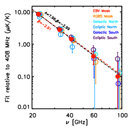
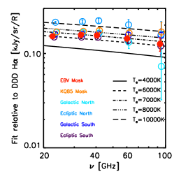
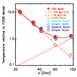
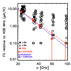
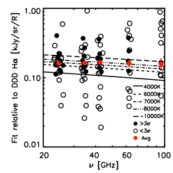
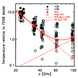
Figure 3: Summary of template fit coefficients. The top row presents results for the full-sky and individual hemispheres, the bottom row shows the values for the 33 regions (after excluding any pixels rejected by the EBV mask). For the regional plots, greater than 3-$\sigma$ detections are shown with filled black circles whilst all other values are shown by open circles. The weighted averages at each frequency of the coefficients for the 33 regions are shown the filled red circles. Left column: Synchrotron - two fits for power-law spectral models are shown; in red the fit includes the 408 MHz reference point, in blue the fit only includes the 5 WMAP frequencies. Neither model includes spectral curvature. Middle column: Free-free - the predicted coefficients (in intensity units) for different electron temperatures as given by Dickinson, Davies & Davis (2003) are shown. Right column: Dust - Straight lines show power spectra fit to the data: in black is a single power law fit to K through Q; in red, two power laws are fit, one with a fixed index of $\beta=1.55$.

4.1 Synchrotron

	Synchrotron spectral indices
Region	K/408	Ka/408	Q/408
EBV	$\bf-2.90^{+0.01}_{-0.01}$	$\bf-2.91^{+0.02}_{-0.02}$	$\bf-2.92^{+0.03}_{-0.03}$
KQ85	$\bf-2.91^{+0.01}_{-0.01}$	$\bf-2.93^{+0.02}_{-0.02}$	$\bf-2.94^{+0.03}_{-0.04}$
NPS	$\bf-3.03^{+0.03}_{-0.03}$	$-3.06^{+0.08}_{-0.12}$	$<-2.90$
GN	$\bf-2.90^{+0.01}_{-0.01}$	$\bf-2.90^{+0.02}_{-0.02}$	$\bf-2.91^{+0.04}_{-0.04}$
GNreduced	$\bf-2.88^{+0.01}_{-0.01}$	$\bf-2.88^{+0.02}_{-0.02}$	$\bf-2.88^{+0.03}_{-0.04}$
EN	$\bf-2.95^{+0.01}_{-0.01}$	$\bf-2.99^{+0.03}_{-0.03}$	$-3.04^{+0.06}_{-0.09}$
ENreduced	$\bf-2.94^{+0.01}_{-0.01}$	$\bf-2.97^{+0.03}_{-0.04}$	$-3.02^{+0.06}_{-0.09}$
GS	$\bf-2.91^{+0.01}_{-0.01}$	$\bf-2.91^{+0.02}_{-0.02}$	$\bf-2.92^{+0.04}_{-0.05}$
ES	$\bf-2.90^{+0.01}_{-0.01}$	$\bf-2.90^{+0.02}_{-0.02}$	$\bf-2.89^{+0.03}_{-0.03}$
1	$<-2.96$	$<-2.88$	$<-2.80$
2	$\bf-2.94^{+0.04}_{-0.05}$	$<-2.79$	$<-2.74$
3	$\bf-3.03^{+0.03}_{-0.03}$	$-3.04^{+0.07}_{-0.10}$	$<-2.89$
4	$<-2.77$	$<-2.60$	$<-2.50$
5	$<-2.75$	$<-2.62$	$<-2.50$
6	$-3.11^{+0.10}_{-0.16}$	$<-2.87$	$<-2.79$
7	$-3.06^{+0.09}_{-0.15}$	$<-2.84$	$<-2.78$
8	$\bf-2.86^{+0.01}_{-0.01}$	$\bf-2.88^{+0.04}_{-0.04}$	$\bf-2.89^{+0.06}_{-0.09}$
9	$-3.15^{+0.09}_{-0.13}$	$<-2.91$	$<-2.84$
10	$\bf-2.90^{+0.06}_{-0.09}$	$-2.76^{+0.08}_{-0.14}$	$-2.64^{+0.08}_{-0.14}$
11	$\bf-2.78^{+0.02}_{-0.03}$	$-2.88^{+0.08}_{-0.14}$	$<-2.76$
12	$\bf-2.92^{+0.06}_{-0.08}$	$<-2.72$	$<-2.63$
13	$<-3.00$	$<-2.93$	$<-2.85$
15	$\bf-2.84^{+0.04}_{-0.04}$	$<-2.78$	$<-2.80$
16	$\bf-2.98^{+0.03}_{-0.03}$	$-2.97^{+0.07}_{-0.09}$	$<-2.82$
17	$\bf-2.94^{+0.04}_{-0.05}$	$<-2.85$	$<-2.82$
18	$\bf-2.90^{+0.06}_{-0.07}$	$<-2.68$	$<-2.59$
19	$<-2.85$	$<-2.67$	$<-2.58$
20	$<-2.82$	$<-2.65$	$<-2.53$
21	$\bf-2.98^{+0.07}_{-0.09}$	$<-2.78$	$<-2.70$
22	$-2.98^{+0.09}_{-0.15}$	$<-2.69$	$<-2.59$
23	$<-2.94$	$<-2.87$	$<-2.81$
24	$\bf-2.80^{+0.04}_{-0.05}$	$-2.71^{+0.07}_{-0.10}$	$-2.65^{+0.08}_{-0.14}$
25	$<-2.92$	$<-2.76$	$<-2.65$
26	$-2.82^{+0.10}_{-0.16}$	$<-2.53$	$<-2.45$
27	$-2.77^{+0.08}_{-0.11}$	$<-2.51$	$<-2.42$
28	$<-2.79$	$<-2.66$	$<-2.57$
29	$-2.80^{+0.10}_{-0.17}$	$<-2.50$	$<-2.40$
30	$<-2.82$	$<-2.67$	$<-2.57$
31	$-2.87^{+0.08}_{-0.13}$	$<-2.70$	$<-2.67$
32	$\bf-2.95^{+0.04}_{-0.04}$	$-2.95^{+0.08}_{-0.14}$	$<-2.76$
33	$-2.89^{+0.08}_{-0.11}$	$<-2.62$	$<-2.52$
Average	$\bf-2.95^{+0.01}_{-0.01}$	$\bf-2.97^{+0.03}_{-0.03}$	$\bf-3.00^{+0.05}_{-0.06}$

Table 1: Synchrotron fits between 408 MHz and WMAP K-, Ka- and Q-bands for various regions of the sky. For those regions that are detected at 2-$\sigma$ significance, the fit values from Table 8 are converted into a spectral index using the usual power-law relation $\beta$ ($T_{b}\propto\nu^{\beta}$). Associated errors are determined by using the fit values plus and minus the 1$\sigma$ error bars. Otherwise, one-sided 95% confidence level upper limits on the index are quoted based on the fit value plus 1.64$\sigma$. Bold text denotes detections at 3-$\sigma$ significance or more. For the global fits, NPS – North Polar Spur, GN – Galactic North, GN_reduced – Galactic North with the NPS removed, EN – Ecliptic North, EN_reduced – Ecliptic North with the NPS removed, GS – Galactic South, ES – Ecliptic South.

As expected, the template fit coefficients between the Haslam 408 MHz data and the WMAP sky maps all fall with frequency in a manner consistent with power-law emission.

In Table 1 we define simple pairwise spectral indices between 408 MHz and the K-, Ka- and Q-bands. The global fits exhibit a typical index of order $-2.90$ at K-band, with the results from all masks slightly flatter than the value of $-3.01$ found in the D06 analysis of the WMAP first-year data for the then-preferred Kp2 sky-coverage. Analyses of the lower-frequency surveys at 408, 1420 and 2326 MHz by Giardino et al. (2002) and Platania et al. (2003) suggest a spectral index over this lower frequency range of approximately $-2.7$, thus our results support the idea of spectral steepening, continuing beyond K-band. We will consider this further in Section 5.

However, there are differences in the coefficients depending on the exact sky coverage that must reflect genuine spectral variations on the sky. The NPS is recognised to be an arc of steep spectrum emission at lower frequencies, thus it is not surprising that it is notably steeper than the rest of the high latitude sky. The spectral index value of $-3.03$ at K-band is quite consistent with the value adopted in Finkbeiner (2004) to remove the prominent emission from the WMAP data. The presence of the NPS also impacts measures of the spectral index in both the Galactic and Ecliptic northern sky, resulting in a modest steepening of the index. Interestingly, the northern Ecliptic hemisphere is notably steeper than the other hemispheres, and exhibits an increasingly steep index with frequency. Conversely, the corresponding southern hemisphere hints at spectral flattening, whereas both the north and south Galactic hemispheres are consistent with simple power-law behaviour.

From the 33 regions of interest, there are 13 regions where the synchrotron fit coefficients are detected at greater than $3\sigma$ confidence at K-band. Most of these regions include contributions close to the Galactic plane, although regions 2, 3 and 32 are mostly at high Galactic latitude. The inferred spectral indices span the range $-2.78$ to $-3.03$, inconsistent with statistical variation alone, and likely representing genuine spectral variations on the sky. We note that region 3 contains the NPS and its behaviour seems to be dominated by that component. Significant emission is detected for region 8 at K-, Ka- and Q-band. Regions 13 and 14 correspond to an area of the sky containing the Gum nebula, and show no evidence for detection of synchrotron emission, with upper limits consistent with a steep spectrum, particularly in the southern region. Interestingly, region 9 has one of the steepest spectral indices on the sky, despite the putative presence of the WMAP haze. However, the overlap between the brightest regions of the haze emission as seen in Dobler & Finkbeiner (2008a) and regions 9, 16 and 17 is very small, and unlikely to affect any studies here.

It is interesting that the spectral indices inferred from the mean of the regional fit coefficients are steeper than the typical global fit values. This trend was also seen in our previous work (D06), and may be due to a selection effect in that the regional subdivisions partly favour stronger synchrotron emission regions which may exhibit steeper spectra than normal due to synchrotron losses. In addition, evidence of spectral steepening with frequency is again generally seen although regions 10 and 24 show inconsistent behaviour with the other regions in that a flattening of the spectrum is indicated.

4.2 Free-free

In this paper, we use an H_α template as a proxy for the free-free emission. We see significant correlation between the WMAP data and the template for the global fits at all frequencies (Table 9). As with the synchrotron results, there are interesting variations depending on the exact sky coverage, with the northern Ecliptic hemisphere showing significantly enhanced amplitude, whilst the south indicates a lower emissivity. 14 individual regions are detected at 3$\sigma$ significance at K-band. Most of these regions lie close to the Galactic plane ($|b|\lesssim 20^{\circ}$).

DDD detail the relationship between the expected free-free brightness temperature and the related H_α intensity, and its dependence on both frequency and electron temperature ($T_{e}$) in the ionised medium. As can be seen from their Fig. 5, the spectral dependence of the emission shows weak curvature, but over the range of frequencies covered by WMAP a reasonable approximation is a power-law with index $-2.15$.

Inspection of the coefficients in Table 9 indicates that there are departures from this behaviour. Following Dobler & Finkbeiner (2008b) we plot these results in intensity units in Fig. 3. It should be apparent that a bump in emission is seen around 40–50 GHz for the global fits, a feature that Dobler & Finkbeiner (2008b) argue is indicative of contributions from both classical free-free emission plus a spinning dust component in the WIM. The mean spectrum of the regional fits perhaps indicates a slightly broader bump in the spectrum. However, it is also the case that there is a range of behaviour seen amongst the individual regions, some of which are consistent with emission from a single physical component only - either free-free emission or a more steeply falling spectrum as expected from spinning dust. In Section 5, we will undertake a more detailed modelling of the emission in terms of these components.

Such a feature in the spectrum of course has implications for the determination of physical parameters such as $T_{e}$. Nevertheless, we can make some general inferences, particularly by examining the K- and W-band amplitudes that are least affected by a putative WIM spinning dust component. The global fits seem to be consistent with values in the range 6000 – 8000 K, with some dependency on the exact mask used. The average free-free electron temperature inferred from the 33 regions is also in this range, although for individual regions there is a spread of values between 4000 and more than 10000 K. These values are somewhat higher than seen previously in Davies et al. (2006), and this is due to the use of 3^∘ smoothed data here, rather than the 1^∘ resolution data used earlier for reasons provided in Appendix A. It is also interesting to note that the 7000 K temperature inferred from the 31.5 GHz $COBE$-DMR data at 7^∘ resolution in Banday et al. (2003) is quite consistent with the Ka-band values determined here. Moreover, the higher values in this paper are in better agreement with the electron temperatures derived from radio recombination line studies of extended HII regions (Shaver et al., 1983; Paladini, Davies & De Zotti, 2004; Alves et al., 2011) which derive an average $T_{e}$ value of $\approx 7000$ K in the vicinity of the solar neighbourhood. There is therefore no need to invoke a large fraction of scattered H_α light to account for this discrepancy (e.g., Witt et al. 2010).

4.3 Impact of Dust Extinction

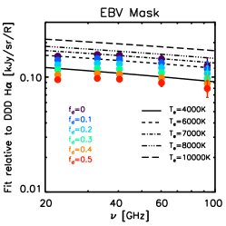
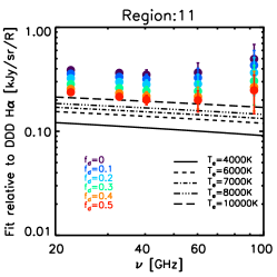
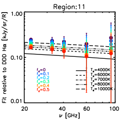
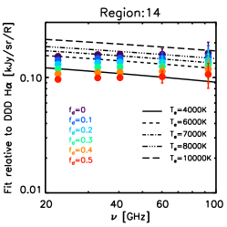
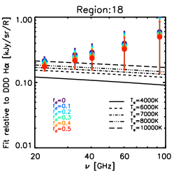
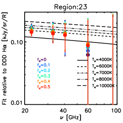
Figure 4: Dependence of the correlation coefficients between the WMAP data and the H_α template as a function of the absorption correction $f_{d}$. The union mask refers to the combination of all 33 small regions defined in this paper. Thus the results for “Union + Galactic North” refers to the inverse-noise-weighted average coefficients for the subset of regions in the northern Galactic hemisphere. The observed dependencies for regions 13, 14 and 23 are representative of that seen for all regions with a significant detection amplitude at K-band.

Bennett et al. (2003b) summarise various uncertainties in the use of the H_α template to trace free-free emission in the Galaxy. These include uncertainties in the value of the electron temperature $T_{e}$, and in the value of the dust absorption correction, specified here by the $f_{d}$ parameter. In principle, there will be variations in both throughout the Galaxy. As noted previously, DDD have determined that for local regions such as Barnard’s Arc and the Gum nebula, there is little absorption by dust, and this is the default situation that we have assumed in our analyses. However, for mid-Galactic latitudes a value $f_{d}\sim$ 0.3 is preferred, and Finkbeiner (2003) adopted the assumption that the H_α emission is co-extensive with dust emission along the line-of-sight, ie. $f_{d}\sim$ 0.5.

In this section we discuss the impact of varying $f_{d}$ on the template fit coefficients. In Fig. 4 we show this variation as a function of $f_{d}$, and compare against the behaviour expected for a range of values of $T_{e}$. In general, we expect that as the amplitude of the H_α template is corrected upwards by increasing $f_{d}$, then the fit coefficients will decrease, implying a lower value for the electron temperature. This is indeed what is seen, but the extent of the correction depends on the region of sky under consideration.

For the largest sky area that we consider, the EBV mask, the use of a template corrected absorption specified by $f_{d}=0.5$ results in coefficients consistent with values of $T_{e}$ of order 3000 K. However, assuming no dust absorption correction yields values closer to 6000 K. A similar result is seen for the southern extension of the Gum nebula (region 14). If it is indeed the case that there is no evidence for dust absorption, then a higher temperature of 6000 K is determined. Conversely, regions 15, 18 and 21 yield coefficients at K-band consistent with temperatures closer to 10000 K if no absorption correction is applied, whereas values of order 8000 K are found for $f_{d}=0.5$. Given that these regions exhibit rising spectra that may require the presence of significant emission from a spinning dust component, then the latter value would be more consistent. However, there are also regions of the sky typified by region 23, where apparently acceptable values of the electron temperature are inferred over a range of values of $f_{d}$. Indeed, it may be that the large spread in coefficients seen for the different regions reflects changes in the fraction of dust mixed with the WIM as much as variations in $T_{e}$.

It does appear, therefore, that there are a range of values for $T_{e}$ and $f_{d}$ throughout the Galaxy, and reaching conclusions about their values solely from studies of H_α correlations suffers from degeneracies between the parameters. The adoption of a value for the dust absorption correction of 0.5 in, for example, Dobler & Finkbeiner (2008b), thus seems to be associated, at least in part, with the low electron temperatures inferred. This uncertainty then has implications for modelling the emission of the diffuse component.

A more serious complication would arise if the validity of using H_α as a tracer of free-free emission were questioned. Mattila, Juvela & Lehtinen (2007) have argued that the H_α excess towards the high-latitude interstellar cloud LDN 1780 is the result of scattering of H_α photons produced elsewhere in the Galaxy by dust in the cloud. Earlier computations by Wood & Reynolds (1999) suggested that this contribution would typically be 5–20% at high-latitudes, although their model has been criticised due to the assumption of a smooth distribution of material in the ISM. Witt et al. (2010) have used an empirical relation to relate the scattered H_α intensity in the translucent cloud LDN1780 to the IRAS 100 $\mu$m diffuse background intensity and conclude that this estimate is reasonable for 50% of the high-latitude sky, but that the scattered contribution can be highly structured and result in contributions of between 25 and 50% of the observed intensity for a further 40% of this region of the sky. Such a result would clearly have implications for using an H_α template to trace free-free emission, and a complex relationship between the template and dust would arise both due to the scattering contribution and due to any dust absorption correction applied to the data. Applying a correction for the former would effectively result in an increase of the H_α-WMAP correlation coefficients and therefore of the inferred electron temperature, whereas application of the latter results in the opposite behaviour. More recently, Brandt & Draine (2011) have estimated the fraction of high-latitude H_α that is scattered to be $19\pm 4\%$, a value consistent with that proposed by Dong & Draine (2011) to reconcile the low ratio of radio free-free to H_α.

Ultimately, unravelling the degeneracy between the electron temperature, H_α scattering and dust absorption requires additional observations. Detailed RRL surveys in the Galactic plane together with radio-continuum surveys at frequencies of $\sim$5 GHz, as expected from the C-BASS (King et al., 2010) will be important in this respect.

Finally, we would like to make some remarks about region 11, the coefficients of which suggest an exceptionally high temperature of more than 25000 K. If this result were considered unphysical, then naively a value of $f_{d}=1$ would be required in order to lower the inferred temperature to the 6000 K seen in the EBV fit. In fact, a more realistic assessment of the situation is that the EBV mask is not large enough to eliminate some parts of region 11 close to the Galactic plane where the simple dust absorption correction is untrustworthy. If instead we apply the KQ85 mask before analysing the region, then for a more plausible value of $f_{d}=0.5$ the inferred electron temperature is again consistent with 6000 K.

4.4 Dust

As can be seen in the right-hand panels of Fig. 3, the template fit coefficients determined between the WMAP data and the FDS8 dust template prediction at W-band are consistent with a rising thermal dust contribution at frequencies higher than V-band, and a rising spectrum to lower frequencies below it. The latter corresponds to the now widely identified anomalous microwave emission (AME).

It appears that the FDS8 template underpredicts the W-band amplitude by approximately 30% for the global fits, consistent with the results of D06. A broad range of values for the individual regions is seen, but only three detect emission at a statistically significant level. The mean emissivity at W-band of all regions shows a more modest enhancement, but is nevertheless consistent with the FDS8 predictions, as indeed are the three significant regions.

At K-band, there are variations in the global fit amplitudes depending on sky coverage. The KQ85 mask indicates a lower emissivity compared to the EBV as might be expected. The Southern Galactic and Ecliptic hemispheres have the highest amplitudes. All coefficients are higher than those determined for the Kp2 sky coverage in D06. 26 of the individual regions detect emission at 3$\sigma$ significance or higher. The mean emission amplitude lies between that for EBV and KQ85, and again somewhat higher than in D06. The regions indicate a variation around the mean of approximately 50% of its amplitude, inconsistent with statistical errors alone and indicating genuine spatial variations in the AME emissivity.

The overall spectrum would appear to be well-described by a superposition of two power-law emissivities. The thermal dust emission described by the FDS8 model is adequately represented by an emissivity index $\beta_{d}=1.55$ over the WMAP range of frequencies. We fit the power-law AME spectrum with the thermal dust index fixed to this value, and find AME spectral indices of order $-2.7$ for both the global fits and regional mean.

Draine & Lazarian (1998a) first proposed that the AME could be explained by electric dipole radiation from rotationally excited small interstellar grains, or spinning dust. Our results have ramifications for such models of the emission. In particular, given that the spinning dust spectra typically fall off steeply with frequency beyond their peak, then it is unlikely that a single such spectrum could account adequately for the effective power-law emission. Indeed, the observed spectrum is presumably formed from a superposition of components with varying spectra as a consequence of their differing physical environments along a given line-of-sight. We will discuss detailed fits of the observed emission in Section 5, and their implications for more refined models of the AME.

5 Model Fits

In order to compare the derived template fit coefficients of a given foreground component with various theoretically motivated foreground models, we adopt the simple procedure used previously in, for example, Dobler & Finkbeiner (2008b). The model parameters of the foreground model are extracted using the least-square minimization defined as,

$$\chi^{2}=\sum_{i}\left[\frac{F(\nu_{i})-F^{M}(\nu_{i})}{\sigma(\nu_{i})}\right]^{2}\,$$

where $F(\nu_{i})$ and $\sigma(\nu_{i})$ are the observed fit coefficients and standard deviation at WMAP frequency bands and $F^{M}(\nu)$ are the fit coefficients given the foreground model. We use a Levenberg-Marquardt method to determine the coefficients, and quote the reduced chi-square for a given model fit. The degree of freedom (dof) is defined as $n-m$ where $n$ represent the number of data points to be fitted and $m$ represents the number of free parameters for a given foreground model. We note that the interpretation of such values can be problematic when the number of data points is small, as is the case here. This is compounded by the correlated errorbars that are dominated by a CMB common to all frequencies. Indeed, the model fits are only to be considered as indicative rather than definitive. A more robust approach would apply a multi-frequency analysis to account for the correlated errors at each frequency due to the dominant CMB term in the covariance matrix. This will form the basis of a future publication where models are fitted directly to the data rather than to previously derived template fit coefficients.

5.1 Spinning Dust preamble

Erickson (1957) first proposed the basic mechanism of spinning dust emission from the rotation of small dust grains with electric dipole moments. Ferrara & Dettmar (1994) later suggested that such grains in the diffuse ionised medium should exhibit significant radio emission peaking at a frequency between 10 and 100 GHz. However, it was Draine & Lazarian (1998a) that suggested such emission could explain the AME, and provided detailed computations of its spectral shape in Draine & Lazarian (1998b).

Indeed, testing for the presence of such emission requires detailed predictions of the emission spectra to compare with observations. However, given the large number of parameters in the model (Ali-Haïmoud, Hirata & Dickinson, 2009), and the fact that most lines-of-sight likely average over many emission regions, this is difficult unless specific objects are considered. Such an analysis was performed recently with early data from the Planck mission (Tauber et al., 2010), specifically for the Perseus and $\rho$-Ophiuchus regions (Planck Collaboration et al., 2011d). Thus, it is usual to adopt spectra for spinning dust in a variety of phases of the ISM, computed for ‘typical’ values of the parameters for those physical conditions. Alternatively, Gold et al. (2009) proposed a generalised analytic form for the spinning dust emission for their analysis of the WMAP 5-year data (see also Bonaldi et al. 2007). However, a fit to the exact CNM form from DL98 underestimates the emission at frequencies beyond the peak. This is problematic given that more recent calculations by Hoang, Draine & Lazarian (2010) indicate that the emission in this region may be broadened by the inclusion of additional physical processes.

We will adopt spinning dust emission templates based on the SPDUST2 code (Silsbee, Ali-Haïmoud & Hirata, 2011) for emission in the cold neutral medium (CNM), warm neutral medium (WNM), and warm ionised medium (WIM). We then allow the spectra to be shifted in both amplitude and peak frequency to fit the data, considering that this approximately mimics the effect of varying the physical parameters as actually required.

5.2 Synchrotron

The following analytic forms are used to fit the synchrotron coefficients.

• Model SI : Given the power law energy distribution of cosmic ray electrons, we assumed a power-law emissivity in terms of brightness temperature over the WMAP frequencies as

  $$T_{A}(\nu)=A_{s}\times\left(\frac{\nu}{23}\right)^{\beta_{s}}_{\text{GHz}}$$ (4)

  where $\beta_{s}$ is the spectral index and $A_{s}$ is the normalised amplitude expressed in $\mu\text{K}$ with respect to the frequency $\nu_{0}=23$ GHz.

• Model SII : A power-law emissivity is assumed to extend from 408 MHz up to and through the WMAP frequencies. Since we use the 408 MHz survey as a template for the synchrotron emission, the amplitude at the low frequency must be reproduced perfectly. This results in an effective constraint to be applied to the analytical form above, and we then fit for the spectral index $\beta_{s}$ only.

  $$T_{A}(\nu)=10^{6}\times\left(\frac{\nu}{0.408}\right)^{\beta_{s}}_{\text{GHz}}$$ (5)

• Model SIII : The cosmic ray electron energy spectrum is expected to steepen with time due to radiation energy loss. A review of cosmic-ray propagation including electrons can be found in Strong, Moskalenko & Ptuskin (2007), whilst Strong, Orlando & Jaffe (2011) directly test propagation models based on cosmic-ray and gamma-ray data against synchrotron data from 22 MHz to 94 GHz as averaged over mid-latitude regions ($10^{\circ}<\mid b\mid<45^{\circ}$). The latter analysis confirms the need for a low-energy break in the cosmic-ray electron injection spectrum to account for the steepening synchrotron spectrum. Since we do not include synchrotron information at frequencies intermediate to 408 MHz and the WMAP data, we follow the treatment of Gold et al. (2009). Specifically, the emissivity is assumed to follow a power-law from 408 MHz until K-band and then to exhibit spectral curvature as follows,

  $$T_{A}(\nu) =A_{s}\times\left(\frac{\nu}{23}\right)_{\text{GHz}}^{\beta_{s}} \nu<\nu_{\text{K}}$$

  $$=A_{s}\times\left(\frac{\nu}{23}\right)_{\text{GHz}}^{\beta_{s}+c_{s}ln(\frac{\nu}{\nu_{\text{K}}})} \nu>\nu_{\text{K}}$$

  As above, the 408 MHz point is fixed, thus $A_{s}$ can be written in terms of $\beta_{s}$, and we are left to fit this spectral index and the curvature $c_{s}$. For a WMAP frequency point, the above equation reduces to the form:

  $$T_{A}(\nu)=10^{6}\times\left(\frac{\nu}{0.408}\right)^{\beta_{s}}_{\text{GHz}}\times\left(\frac{\nu}{23}\right)^{c_{s}ln(\frac{\nu}{\nu_{K}})}_{\text{GHz}}$$ (6)

	SI			SII		SIII
Region	$A_{s}$	$\beta_{s}$	$\chi^{2}$	$\beta_{s}$	$\chi^{2}$	$\beta_{s}$	$c_{s}$	$\chi^{2}$
EBV	7.96 $\pm$ 0.18	-2.99 $\pm$ 0.14	0.047	-2.91 $\pm$ 0.01	0.106	-2.91 $\pm$ 0.01	-0.17 $\pm$ 0.28	0.011
KQ85	7.64 $\pm$ 0.20	-3.11 $\pm$ 0.19	0.246	-2.92 $\pm$ 0.01	0.470	-2.92 $\pm$ 0.01	-0.44 $\pm$ 0.39	0.071
NPS	4.68 $\pm$ 0.55	-3.43 $\pm$ 0.92	0.021	-3.05 $\pm$ 0.03	0.069	-3.04 $\pm$ 0.03	-0.91 $\pm$ 2.18	0.003
GN	8.16 $\pm$ 0.25	-2.94 $\pm$ 0.19	0.007	-2.91 $\pm$ 0.01	0.013	-2.91 $\pm$ 0.01	-0.06 $\pm$ 0.35	0.006
EN	6.41 $\pm$ 0.26	-3.55 $\pm$ 0.33	1.077	-2.97 $\pm$ 0.01	1.914	-2.96 $\pm$ 0.01	-1.38 $\pm$ 0.81	0.628
GS	7.84 $\pm$ 0.26	-2.99 $\pm$ 0.21	0.082	-2.92 $\pm$ 0.01	0.093	-2.92 $\pm$ 0.01	-0.20 $\pm$ 0.42	0.031
ES	7.95 $\pm$ 0.22	-2.74 $\pm$ 0.16	0.337	-2.91 $\pm$ 0.01	0.504	-2.91 $\pm$ 0.01	0.37 $\pm$ 0.23	0.075
2	6.82 $\pm$ 1.25	-3.05 $\pm$ 1.23	0.018	-2.95 $\pm$ 0.04	0.015	-2.95 $\pm$ 0.05	-0.34 $\pm$ 2.59	0.012
3	4.66 $\pm$ 0.53	-3.03 $\pm$ 0.76	0.006	-3.04 $\pm$ 0.03	0.005	-3.05 $\pm$ 0.03	0.08 $\pm$ 1.30	0.005
8	9.23 $\pm$ 0.53	-3.01 $\pm$ 0.38	0.002	-2.88 $\pm$ 0.01	0.037	-2.87 $\pm$ 0.01	-0.25 $\pm$ 0.72	0.005
10	7.67 $\pm$ 2.04	-0.56 $\pm$ 0.42	0.076	-2.86 $\pm$ 0.05	2.305	-2.87 $\pm$ 0.05	1.69 $\pm$ 0.28	0.700
11	12.61 $\pm$ 1.24	-4.33 $\pm$ 1.16	0.560	-2.81 $\pm$ 0.02	1.403	-2.79 $\pm$ 0.03	-3.67 $\pm$ 3.07	0.441
12	7.33 $\pm$ 1.88	-2.09 $\pm$ 1.03	0.028	-2.92 $\pm$ 0.06	0.121	-2.93 $\pm$ 0.06	1.01 $\pm$ 0.88	0.010
15	9.74 $\pm$ 1.62	-5.38 $\pm$ 2.78	1.284	-2.88 $\pm$ 0.04	1.801	-2.85 $\pm$ 0.04	-5.99 $\pm$ 7.08	1.194
16	5.88 $\pm$ 0.62	-2.96 $\pm$ 0.69	0.002	-2.99 $\pm$ 0.03	0.002	-2.99 $\pm$ 0.03	0.01 $\pm$ 1.32	0.002
17	6.42 $\pm$ 1.26	-5.08 $\pm$ 3.08	0.574	-2.98 $\pm$ 0.05	0.822	-2.95 $\pm$ 0.05	-4.99 $\pm$ 7.95	0.527
18	7.95 $\pm$ 1.96	-1.62 $\pm$ 0.77	0.070	-2.89 $\pm$ 0.05	0.373	-2.90 $\pm$ 0.06	1.26 $\pm$ 0.55	0.055
21	5.76 $\pm$ 1.69	-3.18 $\pm$ 1.99	0.001	-2.99 $\pm$ 0.07	0.003	-2.99 $\pm$ 0.07	-0.40 $\pm$ 4.20	0.001
22	5.65 $\pm$ 2.39	-1.44 $\pm$ 1.17	0.031	-2.97 $\pm$ 0.09	0.195	-2.98 $\pm$ 0.09	1.40 $\pm$ 0.83	0.038
24	11.98 $\pm$ 2.20	-1.36 $\pm$ 0.48	0.104	-2.78 $\pm$ 0.04	1.056	-2.79 $\pm$ 0.04	1.27 $\pm$ 0.35	0.231
32	6.64 $\pm$ 0.98	-2.91 $\pm$ 0.93	0.007	-2.96 $\pm$ 0.04	0.006	-2.96 $\pm$ 0.04	0.05 $\pm$ 1.63	0.007

Table 2: Model fits to the synchrotron coefficients determined between the 5 WMAP frequencies and the Haslam 408 MHz template for large sky areas (upper part of table) and for those regions that indicate a 3$\sigma$ significant amplitude at K-band (lower part). The models SI, SII and SIII are described in Section 5.2. $A_{s}$ represents the normalisation amplitude at K-band, $\beta_{s}$ the synchrotron spectral index and $c_{s}$ the spectral curvature. The key for the global fits is as for Table 1.

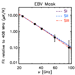
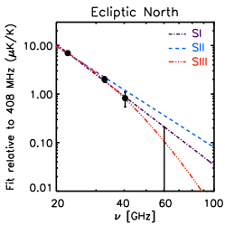
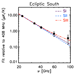
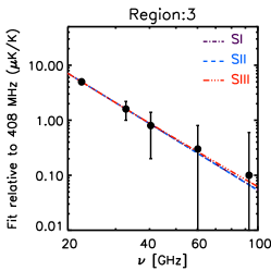
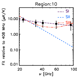
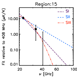
Figure 5: Synchrotron spectral fits for various regions of the sky. A comparison is made of the observed template fits amplitudes derived from the 5 WMAP frequency bands and the 408 MHz survey with the 3 models SI, SII and SIII as defined in Section 5.2. The observed spectral dependencies of regions 3, 10 and 15 are representative of those seen for all regions with a significant detection at K-band.

The results are summarised in Table 2. Fig. 5 presents a comparison of the model fits for three of the global masks, plus three of the regions that can be considered representative of the general results seen. The $\chi^{2}$ results generally should be considered indicative rather than definitive, as would be expected given the small number of data points and the comparable number of model parameters.

The synchrotron fit coefficients obtained for the global masks that include the 408 MHz datum as a reference point (model SII) indicate a typical power-law spectral index of $\beta_{s}=-2.9\pm 0.1$. Model SI fits to the 5 WMAP frequencies are generally steeper, however, only the Ecliptic North region shows evidence of such behaviour at a significant level (a 2$\sigma$ shift in the spectral index). Indeed, a model with negative spectral curvature is the best fit to the data, indicating steepening due to cosmic ray energy loss mechanisms. Curiously, the Ecliptic South indicates spectral flattening, although at much lower significance. The SII fit to the NPS region finds a spectral index $\beta_{s}=-3.05\pm 0.03$ which is steeper than the average spectral index variation over the remaining sky, as expected (Lawson et al., 1987).

For the individual regions, the results are generally similar to the global fits. The spectral behaviour is consistent with emission from power-law cosmic ray electron spectra with only hints of a steepening between 408 MHz and K-band. Region 11 might be considered to show weak evidence for negative spectral curvature. More interestingly, three regions (10, 12 and 24) indicate positive curvature that might be understood as due to the presence of multiple emission regions with varying spectral behaviour along the line-of-sight. However, region 10 has a very flat spectrum between K- and W-band that is strongly favoured over a steeper spectrum extending to 408 MHz, and perhaps even mildly inconsistent with the curvature model adopted here. Whether this indicates some problem with the analysis in this region, due to problems with the templates or cross-talk between components, is difficult to determine. It is apparent that the region lies close to the North Celestial Pole where the 408 MHz template still retains considerable striations from the original survey, whereas we certainly consider that the template fitting methodology has by now been extensively tested. However, the spectral flattening seen in other analyses is less dramatic. For example, Gold et al. (2011) find a range of values of $c_{s}$ between $\pm 0.7$ with a variance of $\sim 0.4$ for their MCMC analysis of the WMAP data combined with the 408 MHz data.

5.3 Free-free

The free-free spectral index is almost constant over the WMAP frequency range and changes only slightly with the the electron temperature. Over this frequency range, the spectral dependence of the corresponding H_α emission can then be approximated with a power-law model of fixed spectral index $-0.15$. However, Dobler & Finkbeiner (2008a) observed deviations from such power-law behaviour, which they attributed to the presence of spinning dust emission in the WIM also traced by H_α. We investigate our template fit coefficients in terms of the following three models.

• Model FI : We consider that the emission is due entirely to the free-free mechanism, ie. a power-law model emissivity with a fixed spectral index of $-0.15$ is assumed,

  $$I(\nu)=A_{f}\times\left(\frac{\nu}{23}\right)^{-0.15}_{\text{GHz}}$$ (7)

  Thus only the free-free amplitude ($A_{f}$) needs to be estimated from the template fit coefficients.
  

• Model FII : The coefficients are fitted with an empirically motivated power-law model emissivity. This is particularly illustrative as to the extent that the standard free-free emissivity index is a poor fit to the data.

  $$I(\nu)=A_{PL}\times\left(\frac{\nu}{23}\right)^{\beta_{PL}}_{\text{GHz}}$$ (8)

  In this case, both the foreground amplitude ($A_{PL}$) and spectral index ($\beta_{PL}$) are to be estimated.
  

• Model FIII : The coefficients are fitted with a combination of free-free emission and a spinning dust model computed by the SPDUST2 code (Silsbee, Ali-Haïmoud & Hirata, 2011) for typical WIM conditions. This model peaks around 30 GHz, but we allow a simple shift $\Delta\nu_{\text{WIM}}$ to be applied to the spectrum, as an approximation that represents the effect of varying the WIM physical parameters to match the model spectrum to the data.

  $$I(\nu)=A_{f}\times\left(\frac{\nu}{23}\right)^{-0.15}_{\text{GHz}}+A_{\text{WIM}}\times D_{\text{WIM}}(\nu-\Delta\nu_{\text{WIM}})$$ (9)

  Here, $D_{\text{WIM}}(\nu)$ represents the normalised spinning dust spectral model for the WIM at a given frequency. Clearly, we must now fit 3 parameters – the free-free amplitude ($A_{f}$), WIM amplitude ($A_{\text{WIM}}$ ) and WIM frequency shift ($\Delta\nu_{\text{WIM}}$). We have also considered fits of this model to the coefficients derived using the H_α after correction for dust absorption ($f_{d}=0.5$).
  

	FI		FII			FIII
Region	$A_{f}$	$\chi^{2}$	$A_{PL}$	$\beta_{PL}$	$\chi^{2}$	$A_{f}$	$A_{WIM}$	$\Delta\nu_{\text{WIM}}$	$\chi^{2}$
EBV	0.156 $\pm$ 0.001	6.374	0.153 $\pm$ 0.002	0.010 $\pm$ 0.036	1.633	0.150 $\pm$ 0.004	2.094 $\pm$ 0.429	13.575 $\pm$ 4.727	0.340
KQ85	0.166 $\pm$ 0.003	2.449	0.163 $\pm$ 0.003	0.061 $\pm$ 0.067	0.205	0.161 $\pm$ 0.004	2.822 $\pm$ 1.204	15.930 $\pm$ 6.463	0.439
GN	0.163 $\pm$ 0.002	2.057	0.161 $\pm$ 0.003	-0.073 $\pm$ 0.065	2.264	0.141 $\pm$ 0.017	3.483 $\pm$ 1.979	5.343 $\pm$ 3.317	0.704
EN	0.210 $\pm$ 0.004	2.177	0.207 $\pm$ 0.004	0.031 $\pm$ 0.070	0.730	0.203 $\pm$ 0.008	3.442 $\pm$ 1.245	14.290 $\pm$ 7.196	0.062
GS	0.156 $\pm$ 0.002	4.622	0.153 $\pm$ 0.002	0.039 $\pm$ 0.044	0.296	0.152 $\pm$ 0.002	2.386 $\pm$ 0.806	16.354 $\pm$ 4.503	1.163
ES	0.146 $\pm$ 0.001	3.499	0.144 $\pm$ 0.002	-0.003 $\pm$ 0.041	1.031	0.141 $\pm$ 0.005	1.775 $\pm$ 0.491	12.932 $\pm$ 6.538	0.202
7	0.126 $\pm$ 0.029	1.003	0.141 $\pm$ 0.030	-2.043 $\pm$ 2.257	0.601	0.000 $\pm$ 0.000	15.936 $\pm$ 3.512	0.000 $\pm$ 0.000	1.381
8	0.111 $\pm$ 0.021	0.086	0.110 $\pm$ 0.024	-0.043 $\pm$ 0.831	0.109	0.053 $\pm$ 0.152	8.168 $\pm$ 18.511	3.214 $\pm$ 10.241	0.024
9	0.162 $\pm$ 0.004	3.619	0.156 $\pm$ 0.004	0.205 $\pm$ 0.101	1.046	0.152 $\pm$ 0.006	5.470 $\pm$ 1.890	15.818 $\pm$ 5.131	0.115
11	0.388 $\pm$ 0.011	0.298	0.386 $\pm$ 0.012	-0.105 $\pm$ 0.128	0.358	0.388 $\pm$ 0.011	0.000 $\pm$ 0.000	0.000 $\pm$ 0.000	0.596
12	0.135 $\pm$ 0.034	0.731	0.150 $\pm$ 0.036	-1.693 $\pm$ 2.087	0.481	0.000 $\pm$ 0.000	17.099 $\pm$ 4.139	0.000 $\pm$ 0.000	0.909
13	0.145 $\pm$ 0.005	0.037	0.145 $\pm$ 0.006	-0.119 $\pm$ 0.169	0.039	0.137 $\pm$ 0.038	1.238 $\pm$ 4.593	4.601 $\pm$ 20.905	0.003
14	0.156 $\pm$ 0.003	2.336	0.153 $\pm$ 0.003	0.060 $\pm$ 0.066	0.096	0.152 $\pm$ 0.003	2.858 $\pm$ 1.513	17.556 $\pm$ 5.663	1.060
15	0.200 $\pm$ 0.011	0.836	0.191 $\pm$ 0.012	0.227 $\pm$ 0.192	0.051	0.192 $\pm$ 0.012	6.819 $\pm$ 6.145	20.334 $\pm$ 7.279	0.627
18	0.235 $\pm$ 0.027	0.772	0.216 $\pm$ 0.029	0.620 $\pm$ 0.358	0.018	0.219 $\pm$ 0.031	19.115 $\pm$ 17.644	21.162 $\pm$ 7.240	0.612
20	0.135 $\pm$ 0.012	1.495	0.123 $\pm$ 0.013	0.685 $\pm$ 0.276	0.116	0.127 $\pm$ 0.014	14.890 $\pm$ 9.172	23.658 $\pm$ 4.864	1.101
21	0.250 $\pm$ 0.043	1.159	0.212 $\pm$ 0.044	1.062 $\pm$ 0.411	0.014	0.222 $\pm$ 0.048	42.774 $\pm$ 29.924	23.582 $\pm$ 5.653	0.893
23	0.164 $\pm$ 0.023	0.157	0.168 $\pm$ 0.025	-0.447 $\pm$ 0.708	0.134	0.066 $\pm$ 0.170	12.174 $\pm$ 20.912	0.000 $\pm$ 0.000	0.144
24	0.118 $\pm$ 0.005	0.340	0.116 $\pm$ 0.006	0.074 $\pm$ 0.195	0.048	0.114 $\pm$ 0.015	1.977 $\pm$ 1.888	13.646 $\pm$ 21.049	0.093
32	0.164 $\pm$ 0.041	0.374	0.144 $\pm$ 0.042	0.914 $\pm$ 0.657	0.019	0.150 $\pm$ 0.046	19.687 $\pm$ 27.751	22.391 $\pm$ 10.970	0.368

Table 3: Model fits to the free-free coefficients determined between the 5 WMAP frequencies and the DDD H_α template for large sky areas (upper part of table) and for those regions that indicate a 3$\sigma$ significant amplitude at K-band (lower part). The models FI, FII and FIII are fully defined in Section 5.3. $A_{f}$ represents the normalisation amplitude of the free-free emission at K-band, $A_{PL}$ represents the normalisation amplitude for the power-law model emission at K-band, $\beta_{PL}$ the corresponding power-law spectral index, $A_{WIM}$ is the amplitude of the WIM spinning dust model in units of 10²⁰ R cm^-2, and $\Delta\nu_{\text{WIM}}$ the shift in frequency of the peak of the dust model to better the fit the data. The key for the global fits as for Table 1.

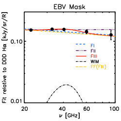
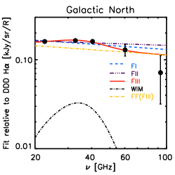
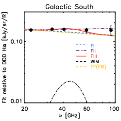
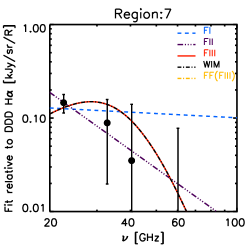
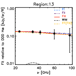
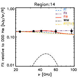
Figure 6: Free-free spectral fits for various regions of the sky. A comparison is made of the observed template fits amplitudes derived from the 5 WMAP frequency bands and the DDD H_α template with the 3 models FI, FII and FIII as defined in Section 5.3. Also shown in the plot are the separate free-free (FF) and WIM spinning dust components that constitute model FIII. The observed spectral dependencies of regions 7, 13 and 14 are representative of those seen for all regions with a significant detection at K-band.

The results are summarised in Table 3. Fig. 6 presents a comparison of the model fits for three of the global masks, plus three of the regions that can be considered representative of the general results seen.

The global fits all indicate a deviation from the free-free emission law (FI) at high significance. Unconstrained power-law fits (FII) are generally flatter, and models containing both free-free and spinning dust emission (FII) are typically preferred. For the EBV mask, the ratio of free-free to spinning dust emission (at the shifted peak frequency) is of order 7, but this drops to 4 for the Galactic North. All regional fits are consistent with a 15 GHz shift to higher frequencies of the peak intensity for the WIM spinning dust component with the exception of the Galactic North region which favours a smaller value of 5 GHz.

The fits to individual regions are generally consistent with the global mask results, and only region 9 shows a clear rejection of model FI. The typical frequency shift is again of order 15 GHz, with a larger dispersion with several regions preferring no shift at all. Of those, regions 7 and 12 can be explained by a single component - either free-free, power-law emission or spinning dust alone with no frequency shift. However, it should be noted that the H_α fit coefficients for these regions are only significant at K-band. Region 11 is consistent with free-free only emission, and yields no evidence for spinning dust, but the region itself has been flagged as anomalous as discussed previously in section 4.3.

Region 13 corresponds to the Northern Gum nebula, and is dominated by free-free emission with a small contribution from spinning dust at a lower peak frequency, $\sim 35$ GHz, than is typical. The Southern part of the nebula is contained in region 14. This is the most clearly detected structure on the sky, significant at all frequencies, as traced by the H_α template, and shows significant evidence for a spinning dust contribution with a free-free to spinning dust ratio of $\sim$ 5. Otherwise, this ratio varies considerably from region to region.

Some regions that have a rising spectrum in terms of the H_α coefficients and naturally favour models with a spinning dust contribution over pure free-free are better fitted still by a flatter/rising power-law emission model. This might be alleviated with more detailed spinning dust modelling (beyond the scope of our paper), or by including physical effects that increase the spinning dust amplitude at frequencies higher than the peak. Such modifications have been investigated by Hoang, Draine & Lazarian (2010).

The $A_{f}$ fit coefficients can, of course, be converted to estimates of the thermal electron temperature in the ionised medium. Since the global mask fits require the presence of a spinning dust component, we only consider the $T_{e}$ results from model FIII, as presented in Table 4. The table also includes results derived from fits to an H_α template corrected for dust absorption assuming $f_{d}=0.5$. We do not include the detailed coefficient results here since the interpretation presented above remains essentially unchanged, and only conclusions about $T_{e}$ are affected. The global masks are consistent with values of the electron temperature of order 6000 K without any dust absorption correction, falling to 3000 K when $f_{d}=0.5$ is assumed. These values are for guidance only – since the regions are not independent, an average is meaningless. It is interesting to note that the Ecliptic North shows an enhanced temperature some 50% higher than these typical values. Whether this reflects some property of the H_α template is difficult to say, but the coverage is dominated by measurements from WHAM data. Conversely, the Ecliptic South global fit gives a lower temperature that may also suggest issues with the template, given that it is largely comprised of the SHASSA fields. New observations from the southern extension of the WHAM survey (Haffner et al., 2010) should help resolve this issue in the near future. Nevertheless, problems may still remain near the ecliptic poles given difficulties with removing the geocoronal H_α contribution. For the individual regions (ignoring region 11 which is considered to be anomalous), we find a weighted average of $6300\pm 200$ K (dropping to 5900 K if region 11 is excluded) without a correction for dust absorption, and $2900\pm 100$ K otherwise. These values are in good agreement with the global averages as might be expected. However, note that the dispersion of values is considerably larger than the quoted uncertainty, implying true variations in temperature on the sky. Moreover, as discussed previously, it is likely that some of the dispersion seen reflects the existence of a range of values for both $T_{e}$ and $f_{d}$ throughout the Galaxy.

	Inferred $T_{e}$ (K) for model FIII
Region	$f_{d}=0.0$	$f_{d}=0.5$
EBV	5900 $\pm$ 300	2600 $\pm$ 200
KQ85	6600 $\pm$ 300	3200 $\pm$ 200
GN	5300 $\pm$ 1000	2500 $\pm$ 500
EN	9500 $\pm$ 600	5300 $\pm$ 600
GS	6000 $\pm$ 100	2600 $\pm$ 100
ES	5300 $\pm$ 300	2200 $\pm$ 200
7(a)	4400 $\pm$ 1700	5600 $\pm$ 1100
8(a)	3600 $\pm$ 1200	2300 $\pm$ 900
9	6000 $\pm$ 400	3200 $\pm$ 300
11	25500 $\pm$ 1100	11800 $\pm$ 500
12(a)	5000 $\pm$ 2100	3300 $\pm$ 1300
13	5100 $\pm$ 2200	3500 $\pm$ 1500
14	6000 $\pm$ 200	2700 $\pm$ 100
15	8600 $\pm$ 800	5900 $\pm$ 600
18	10700 $\pm$ 2300	7700 $\pm$ 1700
20	4500 $\pm$ 800	2400 $\pm$ 500
21	10900 $\pm$ 3600	4000 $\pm$ 1800
23(a)	6800 $\pm$ 1400	5400 $\pm$ 1000
24	3700 $\pm$ 600	2300 $\pm$ 700
32	5900 $\pm$ 2900	5600 $\pm$ 2500

Table 4: Inferred free-free electron temperature $T_{e}$ in Kelvins corresponding to model fit FIII with dust corrections $f_{d}=0.0$ and $0.5$. ${}^{(}a)$ These regions show an effective degeneracy between free-free only or WIM spinning dust only solutions, thus FIII solutions have no contribution from free-free emission. We have therefore used the FI results to compute $T_{e}$ in these cases.

5.4 Dust

The total dust emission is modelled as a combination of the relatively well-understood thermal dust emission and the AME. The former is assumed to have a fixed spectral index relative to the FDS8 94 GHz template over the WMAP frequency range as determined directly from the FDS8 model. We consider the following two models in order to fit the dust coefficients.

• Model DI : The dust coefficients are fitted with a combination of thermal (vibrational) dust and a power law dust-correlated AME.
  

  $$T_{A}(\nu)=A_{PLD}\times\left(\frac{\nu}{23.}\right)^{\beta_{PLD}}_{\text{GHz}}+A_{TD}\times\left(\frac{\nu}{94}\right)^{1.55}_{\text{GHz}}$$ (10)

  Three parameters – the thermal dust amplitude ($A_{TD}$), the power law dust amplitude ($A_{PLD}$) and power law dust spectral index ($\beta_{PLD}$) – are fitted to the coefficients.

• Model DII : The dust coefficients are fitted with a combination of thermal dust and two spinning dust components (CNM and WNM). The two spectra are generated using the SPDUST2 code assuming typical CNM and WNM conditions (Draine & Lazarian, 1998a). Given that both spectra peak at approximately the same frequency ($\approx 30$ GHz), and the limited number of degrees of freedom available in the fit, it is only possible to apply a frequency shift to one component in order to match observations. Hoang, Lazarian & Draine (2011) found that modifying the CNM properties to increase its peak frequency yields a closer match to the WMAP observations, and therefore we elect to allow a frequency shift of this component.
  

  $$T_{A}(\nu)=A_{\text{WNM}}\times D_{\text{WNM}}(\nu)+A_{\text{CNM}}\times D_{\text{CNM}}(\nu-\Delta\nu_{\text{CNM}})+A_{TD}\times\left(\frac{\nu}{94}\right)^{1.55}_{\text{GHz}}$$ (11)

  We fit four parameters to the template fit coefficients: the thermal dust amplitude ($A_{TD}$), the WNM amplitude ($A_{\text{WNM}}$) normalised at 23 GHz, the CNM amplitude ($A_{\text{CNM}}$) normalised at 41 GHz, and the CNM peak frequency shift ($\Delta\nu_{\text{CNM}}$).

Region	Model DI				Model DII
	$A_{PLD}$	$\beta_{PLD}$	$A_{TD}$	$\chi^{2}$	$A_{WNM}$	$A_{CNM}$	$\Delta{\nu_{\text{CNM}}}$	$A_{TD}$	$\chi^{2}$
EBV	9.15 $\pm$ 0.09	-2.74 $\pm$ 0.06	1.01 $\pm$ 0.08	1.710	9.35 $\pm$ 0.10	0.67 $\pm$ 0.09	22.42 $\pm$ 1.22	1.22 $\pm$ 0.08	0.825
KQ85	7.61 $\pm$ 0.08	-2.78 $\pm$ 0.07	1.14 $\pm$ 0.08	0.667	7.78 $\pm$ 0.09	0.53 $\pm$ 0.08	23.34 $\pm$ 1.33	1.29 $\pm$ 0.08	1.208
GN	8.91 $\pm$ 0.14	-2.86 $\pm$ 0.11	1.00 $\pm$ 0.13	0.769	9.12 $\pm$ 0.15	0.50 $\pm$ 0.14	23.35 $\pm$ 2.51	1.18 $\pm$ 0.13	0.829
EN	8.32 $\pm$ 0.13	-2.83 $\pm$ 0.11	0.99 $\pm$ 0.13	0.617	8.51 $\pm$ 0.14	0.49 $\pm$ 0.14	23.35 $\pm$ 2.42	1.16 $\pm$ 0.13	0.679
GS	9.73 $\pm$ 0.13	-2.64 $\pm$ 0.08	1.02 $\pm$ 0.13	0.699	9.93 $\pm$ 0.13	0.85 $\pm$ 0.13	21.99 $\pm$ 1.41	1.28 $\pm$ 0.12	0.114
ES	9.82 $\pm$ 0.13	-2.69 $\pm$ 0.08	0.99 $\pm$ 0.12	1.162	10.01 $\pm$ 0.13	0.78 $\pm$ 0.12	22.07 $\pm$ 1.47	1.24 $\pm$ 0.11	0.285
2	8.03 $\pm$ 1.60	-4.14 $\pm$ 2.16	0.00 $\pm$ 0.00	0.093	8.17 $\pm$ 1.63	0.00 $\pm$ 0.00	0.00 $\pm$ 0.00	0.00 $\pm$ 0.00	0.378
3	8.73 $\pm$ 0.99	-2.60 $\pm$ 0.66	2.03 $\pm$ 0.95	0.016	8.94 $\pm$ 1.04	0.88 $\pm$ 0.97	23.97 $\pm$ 8.94	2.20 $\pm$ 0.91	0.001
6	7.49 $\pm$ 2.33	-3.06 $\pm$ 2.31	0.84 $\pm$ 2.20	0.007	7.68 $\pm$ 2.44	0.17 $\pm$ 2.50	25.27 $\pm$ 100.72	0.99 $\pm$ 2.23	0.002
7	9.79 $\pm$ 0.63	-2.56 $\pm$ 0.40	1.19 $\pm$ 0.64	0.034	9.96 $\pm$ 0.67	0.98 $\pm$ 0.65	21.14 $\pm$ 6.79	1.49 $\pm$ 0.60	0.008
8	6.70 $\pm$ 0.63	-2.73 $\pm$ 0.62	1.41 $\pm$ 0.62	0.019	6.86 $\pm$ 0.66	0.56 $\pm$ 0.68	24.81 $\pm$ 8.69	1.48 $\pm$ 0.61	0.018
9	13.09 $\pm$ 0.45	-2.61 $\pm$ 0.22	1.09 $\pm$ 0.52	0.121	13.34 $\pm$ 0.48	1.20 $\pm$ 0.48	21.58 $\pm$ 3.83	1.49 $\pm$ 0.50	0.003
10	6.55 $\pm$ 0.71	-3.16 $\pm$ 0.76	0.67 $\pm$ 0.60	0.051	6.69 $\pm$ 0.74	0.11 $\pm$ 0.70	25.45 $\pm$ 44.79	0.78 $\pm$ 0.61	0.110
11	4.20 $\pm$ 0.63	-2.45 $\pm$ 0.84	0.81 $\pm$ 0.64	0.061	4.21 $\pm$ 0.86	0.44 $\pm$ 0.59	16.51 $\pm$ 25.45	1.02 $\pm$ 0.59	0.006
12	5.29 $\pm$ 0.36	-3.79 $\pm$ 0.68	0.35 $\pm$ 0.38	0.304	5.40 $\pm$ 0.37	0.00 $\pm$ 0.00	0.00 $\pm$ 0.00	0.34 $\pm$ 0.35	1.691
13	5.61 $\pm$ 0.71	-3.16 $\pm$ 0.88	0.78 $\pm$ 0.60	0.048	5.73 $\pm$ 0.75	0.09 $\pm$ 0.69	24.66 $\pm$ 62.57	0.88 $\pm$ 0.61	0.091
14	9.70 $\pm$ 0.45	-2.53 $\pm$ 0.28	1.20 $\pm$ 0.43	0.033	9.87 $\pm$ 0.48	1.03 $\pm$ 0.46	21.51 $\pm$ 4.49	1.50 $\pm$ 0.40	0.000
15	8.25 $\pm$ 0.54	-2.41 $\pm$ 0.38	1.64 $\pm$ 0.55	0.015	8.40 $\pm$ 0.58	1.06 $\pm$ 0.56	21.79 $\pm$ 5.14	1.92 $\pm$ 0.50	0.037
16	6.29 $\pm$ 0.62	-4.72 $\pm$ 1.36	0.00 $\pm$ 0.00	0.327	6.38 $\pm$ 0.63	0.00 $\pm$ 0.00	0.00 $\pm$ 0.00	0.00 $\pm$ 0.00	3.088
17	6.59 $\pm$ 1.79	-3.90 $\pm$ 2.82	0.17 $\pm$ 1.62	0.055	6.73 $\pm$ 1.83	0.00 $\pm$ 0.00	0.00 $\pm$ 0.00	0.15 $\pm$ 1.52	0.148
18	6.99 $\pm$ 0.90	-3.41 $\pm$ 1.10	0.57 $\pm$ 0.78	0.053	7.14 $\pm$ 0.91	0.00 $\pm$ 0.00	0.00 $\pm$ 0.00	0.67 $\pm$ 0.72	0.127
19	9.29 $\pm$ 1.88	-1.87 $\pm$ 0.99	2.81 $\pm$ 2.23	0.050	9.48 $\pm$ 2.01	2.19 $\pm$ 1.97	22.96 $\pm$ 7.81	3.36 $\pm$ 1.81	0.062
20	9.85 $\pm$ 0.72	-2.90 $\pm$ 0.52	0.87 $\pm$ 0.71	0.070	10.09 $\pm$ 0.76	0.45 $\pm$ 0.76	23.50 $\pm$ 14.84	1.08 $\pm$ 0.71	0.024
21	6.92 $\pm$ 0.45	-2.98 $\pm$ 0.47	0.96 $\pm$ 0.40	0.049	7.08 $\pm$ 0.47	0.28 $\pm$ 0.47	24.34 $\pm$ 12.08	1.08 $\pm$ 0.41	0.124
22	8.73 $\pm$ 0.81	-2.40 $\pm$ 0.54	1.69 $\pm$ 0.87	0.019	8.87 $\pm$ 0.87	1.08 $\pm$ 0.85	20.69 $\pm$ 8.30	2.03 $\pm$ 0.80	0.023
23	8.96 $\pm$ 0.36	-2.54 $\pm$ 0.22	1.12 $\pm$ 0.32	0.079	9.12 $\pm$ 0.38	0.95 $\pm$ 0.30	21.38 $\pm$ 3.44	1.40 $\pm$ 0.30	0.005
24	7.75 $\pm$ 0.54	-3.56 $\pm$ 0.63	0.04 $\pm$ 0.49	0.207	7.92 $\pm$ 0.55	0.00 $\pm$ 0.00	0.00 $\pm$ 0.00	0.10 $\pm$ 0.45	0.867
28	8.46 $\pm$ 1.80	-2.03 $\pm$ 1.09	2.47 $\pm$ 2.01	0.038	8.64 $\pm$ 1.91	1.73 $\pm$ 1.89	23.34 $\pm$ 9.27	2.83 $\pm$ 1.71	0.031
30	9.73 $\pm$ 3.14	-2.00 $\pm$ 1.62	2.30 $\pm$ 3.47	0.006	9.85 $\pm$ 3.36	2.09 $\pm$ 3.18	21.92 $\pm$ 14.67	2.81 $\pm$ 2.91	0.002
31	12.00 $\pm$ 3.23	-1.93 $\pm$ 1.32	2.70 $\pm$ 3.66	0.005	12.13 $\pm$ 3.46	2.67 $\pm$ 3.27	21.47 $\pm$ 12.17	3.45 $\pm$ 3.00	0.011
32	8.15 $\pm$ 0.81	-2.87 $\pm$ 0.70	0.85 $\pm$ 0.81	0.003	8.33 $\pm$ 0.85	0.53 $\pm$ 0.87	24.26 $\pm$ 12.86	0.95 $\pm$ 0.81	0.098
33	8.53 $\pm$ 1.88	-3.08 $\pm$ 1.60	0.78 $\pm$ 1.70	0.025	8.74 $\pm$ 1.99	0.12 $\pm$ 1.91	23.77 $\pm$ 135.62	0.99 $\pm$ 1.72	0.004

Table 5: Model fits to the dust coefficients determined between the 5 WMAP frequencies and the FDS8 template for large sky areas (upper part of table) and for those regions that indicate a 3$\sigma$ significant amplitude at K-band (lower part). The models DI and DII are fully defined in Section 5.4. $A_{PLD}$ and $\beta_{PLD}$ represent the normalisation amplitude at K-band and spectral index respectively of a power-law anomalous dust emission component. $A_{WNM}$ is the amplitude of the WNM spinning dust model at K-band, $A_{CNM}$ is the amplitude of the CNM spinning dust model normalised at 41 GHz, and $\Delta\nu_{CNM}$ is the shift in frequency of the peak of the CNM dust model to better the fit the data. $A_{TD}$ is the amplitude of the thermal dust emission with an assumed spectral index $\beta_{TD}=1.55$ as determined directly from the FDS8 dust model. The key for the global fits as for Table 1.

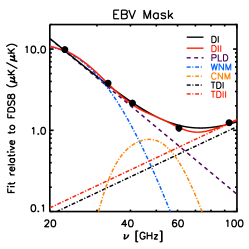
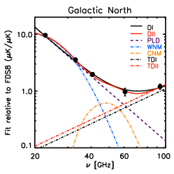
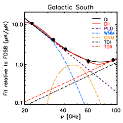
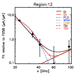
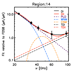
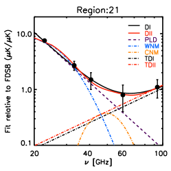
Figure 7: Dust spectral fits for various regions of the sky. A comparison is made of the observed template fit amplitudes derived from the 5 WMAP frequency bands and the FDS8 template with the 2 models DI and DII as defined in Section 5.4. Also shown in the plot are the separate power-law anomalous dust (PLD) and vibrational (thermal) dust (VD) that constitute model DI, and the cold neutral medium (CNM) and warm neutral medium (WNM) components that, together with the vibrational dust, constitute model DII. The observed spectral dependencies of regions 12, 14 and 21 are representative of those seen for all regions with a significant detection at K-band.

The results are summarised in Table 5. Fig. 7 presents a comparison of the model fits for three of the global masks, plus three of the regions that can be considered representative of the general results seen.

It should be apparent from the table that both models DI and DII provide adequate fits to the global masks. However, in order to explain the emission at V-band in terms of spinning dust models, two contributions are required in combination with an enhanced thermal dust normalisation some 20% larger than that predicted at 94 GHz by FDS8. Such models also require a shift in the peak CNM emission of $\sim$22 GHz and a ratio of WNM to CNM spinning dust emission of order 4:1. In fact, if the CNM emission were to be omitted, or the thermal dust amplitude kept at the canonical FDS8 value, then the V- and/or W-band amplitudes would be substantially underpredicted. In practise, given the low number of data points sensitive to the thermal dust emission, there is an effective degeneracy between the CNM and vibrational dust components, that may be alleviated somewhat if the spinning dust models can be enhanced in amplitude at frequencies higher than their peak. Indeed, spinning dust can contribute significantly to emission in the $\sim$60 to 90 GHz range depending on the local physical conditions. However, one might then expect to see a much flatter spectrum around the Q-, V-, and W-bands than is actually observed. It may also be that some modification of the assumed thermal dust spectral index is required.

The fits to individual regions are less informative, as expected given the lack of clear detections for the template fit coefficients at V- and W-band. Given this, the analysis might be criticised for overfitting the data points. Nevertheless, both a power-law and a WNM spinning dust component are good candidates to explain the lower frequency points. In almost all cases, a significant contribution from CNM or thermal dust emission is not required. This discrepancy between the regional fits and global analysis may simply reflect a signal-to-noise issue at higher frequencies than the former, or the fact that the latter are essentially averages over many regions which exhibit some variation in dust properties. Regions 12 and 16 are interesting in that the power-law model is clearly preferred over model DII, although the analysis is really only constrained by the data points at K- and Ka-band. For those regions in which a significant vibrational dust contribution is required, the amplitude is systematically higher than the canonical FDS8 value, although still consistent with it. However, the required DI enhancement is lower, thus the DII results more likely again point to a deficiency in the specific spinning dust models used in this analysis.

The FDS8 model value for the dust spectral index used here is quite flat, whereas early Planck papers (Planck Collaboration et al., 2011b, a) studying emission at frequencies higher than $\sim$100 GHz favour values closer to 1.8. However, Planck Collaboration et al. (2011c) suggests that the dust SED flattens in the millimetre wavelength range. At lower frequencies, there is considerable uncertainty, and detailed modelling for candidate AME regions (including Perseus and $\rho$-Ophiucus) of the foreground spectra for all components and across the Planck frequencies suggests values in the range 1.5–2 (Planck Collaboration et al., 2011d). We have repeated the calculations above but imposing a thermal dust spectral index of 1.7 on the fits. For model DI, there is a general increase in amplitude of the power-law dust component, with an associated flattening of the spectral index at levels below the 1-$\sigma$ error bar, and no impact on the thermal dust amplitude. Model DII shows similarly modest increases in the amplitudes of the two spinning dust components, with little change in the CNM peak frequency shift, and again no change in the thermal dust amplitude. However, adopting the FDS8 thermal dust model at W-band and then imposing a steeper index to lower frequencies is not self-consistent. Therefore, a more detailed treatment is required including specific modelling of all dust components combined with higher frequency measurements. An obvious potential error in our analysis is the selective use of the CNM and WNM spectra for typical conditions in those phases of the ISM. What is clear is that the frequency range of 60–100 GHz is a remarkably interesting regime for dust astrophysics.

6 Discussion

In our study of the free-free, dust and synchrotron foreground components in the WMAP data, we have selected fields based on the morphological properties of three templates that trace the emission at wavelengths where the emission mechanism is (largely) dominant, and we assume that such partitions correlate well with spectral behaviour. Each of these components has then been quantified in terms of a mean value of the emissivity in each of the 5 WMAP bands.

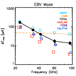
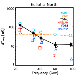
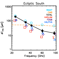
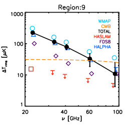
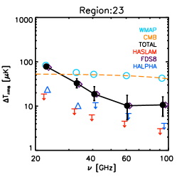
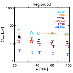
Figure 8: R.M.S amplitude in antenna temperature observed for various regions of the sky. The signal associated with the total foreground is shown as black filled circles. The synchrotron contribution traced by the Haslam template is represented by red squares, the free-free traced by the H_α template as dark blue triangles, and the dust contribution traced by the FDS8 template as purple diamonds. One-sided 95% c.l. upper limits are shown for non-detections, with the appropriate colour coding for the component represented. The r.m.s. amplitude of the uncorrected WMAP frequency maps is indicated by open light blue circles. The orange line corresponds to the CMB level estimated from the 7-year ILC map. The observed spectral shapes of regions 9, 23 and 33 are representative of those seen for all regions.

In Fig. 8, we show the r.m.s contributions of the foregrounds in antenna temperature as traced by the templates for three of the global fits and a representative set of the regional results. These values were derived from the template r.m.s values as recorded in Table 6 and scaled appropriately by the fit coefficients from our analysis. For comparison, we show the uncorrected r.m.s. amplitude at each WMAP frequency, together with an estimate of the CMB fluctuations from the ILC sky map, all determined for the same sky coverage as the foregrounds. We assume that this template based technique traces essentially all of the foreground contribution, and this may not be the case. In particular, we recognise the WMAP-haze (Finkbeiner, 2004; Dobler & Finkbeiner, 2008a) as an important exception. Nevertheless, our interpretations should remain robust.

	r.m.s amplitude
Region	408 MHz (K)	Hα (R)	FDS8 ($\mu$K)
EBV	10.91	9.30	10.21
KQ85	9.44	3.75	11.44
GN	10.74	6.18	9.79
EN	9.97	3.71	10.14
GS	11.08	11.56	10.52
ES	11.60	12.27	10.27
1	3.17	0.16	0.93
2	6.27	0.67	3.57
3	10.96	0.49	4.27
4	1.59	0.14	0.95
5	1.27	0.09	1.07
6	5.86	0.35	2.95
7	5.49	1.75	5.61
8	15.77	2.81	6.92
9	4.96	20.19	7.19
10	3.32	0.86	8.28
11	6.51	5.60	8.99
12	4.98	1.19	6.97
13	5.08	11.97	8.32
14	3.98	37.92	12.22
15	4.22	5.34	9.01
16	13.27	1.12	8.42
17	5.39	1.15	3.06
18	3.68	2.90	7.09
19	2.23	1.95	3.79
20	2.81	5.68	5.61
21	4.89	1.61	7.08
22	4.00	1.21	6.55
23	2.58	2.19	7.75
24	3.14	8.29	5.83
25	1.89	0.28	1.86
26	0.98	0.13	0.55
27	0.77	1.06	1.24
28	0.88	0.15	2.02
29	0.97	0.15	0.51
30	1.70	0.08	1.81
31	1.59	0.19	1.30
32	5.03	0.31	3.02
33	1.47	0.17	2.20

Table 6: R.m.s amplitudes of the foreground templates. These values are scaled to the WMAP frequencies using the fit coefficients in Tables 8, 9 and 10.

Note that the spectral shape of the integrated foregrounds, where determined, is relatively simple when sparsely sampled by the WMAP frequencies, but nevertheless it is interesting that a simple power-law frequency dependence, or only modest deviations therefrom, is needed to describe the emission from K- to V-band. This observation was central to the work of Park, Park & Gott (2007) in partitioning the sky to perform local CMB reconstruction.

For the EBV mask, it is clear that the foregrounds as traced by three templates are of similar amplitude at K-band, and the free-free and dust contributions remain roughly equal to V-band, whereas the synchrotron falls off more steeply. The foregrounds remain comparable to, or larger than, the CMB fluctuations to Q-band, and significant at V- and W-bands.

Comparing the total foreground contributions between the North and South Ecliptic hemispheres, it can be observed that the amplitude is higher in the South at least from K- to V-band. It also appears that the free-free component shows a particular enhancement in the South. Whether this may be connected to problems in the H_α template (see Appendix A for details) might be discussed. However, the foreground differences are interesting in the context of the hemispherical asymmetry seen in the distribution of power in the CMB in Ecliptic coordinates, as noted originally by Park (2004); Eriksen et al. (2004) and revisited many times in the literature (see Copi et al., 2010, for a review). Indeed, the r.m.s. CMB signal plotted here clearly shows this asymmetry. Specifically, if the foregrounds were underestimated in the Northern hemisphere (as might be the case for the free-free component), then correcting for this effect would only exacerbate the problem. A similar consequence results from an overestimate of the foregrounds in the South. Thus, it seems unlikely that the CMB asymmetry is connected with problems of Galactic foreground estimation, as noted before in Hansen et al. (2006).

As expected, there are also clear variations between the regions used in our study. Region 9 represents a region with strong foreground contributions at all frequencies, the dominant contribution being from the free-free emission. Region 23 is a dust dominated region, but the significance of the contamination relative to the CMB is lower, although the dust is detected clearly at all frequencies. Finally, region 33 typifies many high- and mid-latitude regions where foregrounds are only detected, if at all, at K- and possibly Ka-band. The amplitude of the 95% upper limits combined with the agreement between the uncorrected frequency maps and the CMB estimate from the ILC implies that foregrounds are essentially unimportant in these regions.

There are several interesting aspects of the study with regards to the properties of the foregrounds that should be highlighted. The synchrotron emission shows clear evidence of steepening relative to measures at GHz frequencies. There is a hint of this steepening continuing beyond K-band. The temperature of the electrons responsible for the free-free emission is now much more consistent with other indicators such as RRLs, ie. $\sim$7000 K at high latitudes. This result is in part due to an improved understanding of the H_α template. This clearly needs to be improved and will benefit greatly from the WHAM-S survey when available. However, uncertainties related to the dust absorption remain. The AME is essentially ubiquitous, comparable in amplitude to the free-free emission, and with a spectrum broader than a single component. There does appear to be an additional anomalous component correlated with the H_α emission, but there are variations in relative strength on the sky. An improved model of the AME requires an improvement in the understanding of the corresponding thermal dust contribution. Specifically, the emissivity of the thermal dust tail to low frequencies must be determined, and a detailed model of the emissivity as a function of wavelength and dust temperature needs to be derived from the data.

Finally, we note that studies of foregrounds at microwave wavelengths using the techniques in this paper are essentially limited by the quality and resolution of the available templates. A comparison of synchrotron and free-free properties over the full-sky are, at best, possible on angular scales of 1^∘ and above, given the resolutions of the 408 MHz and H_α data. Moreover, we have noted some problems with the H_α template on scales less than 3^∘. However, this should not limit the analysis of Planck data, and especially that from the high-frequency instrument (HFI) operating at frequencies above 100 GHz, which will determine the R-J tail of thermal dust emission. Similarly, data at frequencies $\sim 5-20$ GHz will help determine the complicated mix of low frequency foregrounds. For example, there could be a possible contribution from synchrotron radiation with a flatter spectral index compared to the values determined from correlations with 408 MHz data. We note that a recent study by Peel (2011) who used a 2.3 GHz survey of the southern sky found that the AME was relatively unaffected limiting the contribution of such a component to $\sim 7\,\%$ of the AME at 23 GHz.

7 Acknowledgements

Some of the results in this paper have been derived using the HEALPix package (Górski et al., 2005). We acknowledge the use of the Legacy Archive for Microwave Background Data Analysis (LAMBDA). Support for LAMBDA is provided by the NASA Office of Space Science. CD acknowledges an STFC Advanced Fellowship and ERC IRG grant under the FP7.

Appendix A H_α Templates

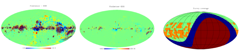
Figure 9: Left and middle: difference map between the DDD and F03 H_α templates. The F03 map has been additionally smoothed by a Gaussian beam of $(60^{2}-6^{2})^{1/2}$ degrees so that the two sky maps have a matched 1^∘ resolution. The two plots are identical except for the color scale. Right: the coverage of the different datasets used in the two templates. In light green is where both templates use WHAM data, and in red where both use SHASSA data. Orange shows where the F03 template uses VTSS data. In dark blue is the region where DDD uses WHAM data while F03 uses SHASSA.

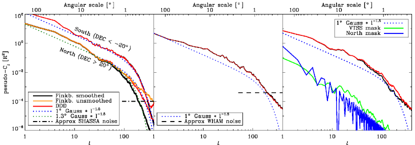
Figure 10: Pseudo-$C_{\ell}$ spectra computed from the DDD and F03 H_α templates. Left: pseudo-$C_{\ell}$ spectra of discs centered on either Celestial North or South ($|\delta|>20\degr$). Dashed lines show the Southern spectra while solid the Northern. Results from the DDD template are shown in red, those from the F03 map smoothed to 1^∘ resolution are in black, and in orange we show results from the F03 template without additional smoothing. Dotted lines give simple power law spectra smoothed with Gaussian beams of 1$\degr$ (1.3$\degr$) in blue (green) with arbitrary power law indices and amplitudes fit by eye solely for visual comparison. Middle: pseudo-$C_{\ell}$ spectra of sky regions where both F03 and DDD templates use only WHAM data. The F03 template has been smoothed as described in the text. Right: pseudo-$C_{\ell}$ spectra of sky regions where F03 uses VTSS data but DDD uses WHAM. For comparison, the pseudo-$C_{\ell}$s for the masks themselves are shown, the VTSS used for the red and black curves, and the North mask used in the top figure. The effects of the highly structured VTSS mask dominates toward high $\ell$, which makes the lower two plots difficult to compare with the top plot, where an azimuthally symmetric mask does not impact the power spectrum. But it is apparent that the differences in the north are due to the use of the VTSS data.

We have compared the DDD and Finkbeiner (2003, hereafter F03) H_α templates and performed template fits to the WMAP data using both for comparison. As in D06, there are sometimes significant differences in the resulting cross-correlation coefficients, that we previously ascribed to an inaccuracy in our knowledge of the WHAM effective beam. Here, we investigate the detailed differences between the templates themselves.

The DDD template used a combination of WHAM data in the north and SHASSA data in the south, with preference for the WHAM data down to a declination of $-10\degr$. F03 chose to use SHASSA data wherever it was available, augmented by data from the Virginia Tech Spectral-line survey (hereafter VTSS, Dennison, Simonetti & Topasna, 1998), a complementary narrow-band imaging survey which covers the northern sky for $\delta\geq-15^{\circ}$, and has an angular resolution of 1.6 arc minute. The SHASSA data were processed differently, and different methods used to adjust the resolutions of these datasets for consistency and merging. The DDD template claims a nominal resolution of 1$\degr$ FWHM, while the F03 template has a stated resolution of 6$\arcmin$.

Fig. 9 shows the differences between the two maps on two different color scales to bring out the small and large amplitude differences. Clearly, the processing differences result in maps that differ at the roughly 1 Rayleigh (R) level over large regions of the sky, and of more than 20 R level near very bright regions, although the latter are generally excluded by our EBV and KQ85 masks.

To investigate the properties of these templates further, we have computed pseudo-C_ℓ power spectra in the Celestial North and South where the DDD template uses exclusively WHAM or SHASSA data, respectively. The results are shown in Fig. 10. The noise properties of the maps are difficult to quantify because many components can contribute, including stellar residuals that will dominate. However, the instrumental thermal noise is approximately known. For the WHAM survey, the noise level varies over the sky but is typically 0.02 R, whereas for SHASSA the corresponding amplitude is $\sim$ 0.01 R. These values are overplotted in the figure. In the case of the DDD template, no additional smoothing has been applied, but for the F03 map we have smoothed the data from the stated resolution of $6\arcmin$ to a $1^{\circ}$ effective FWHM. It is interesting to note the asymmetry in amplitudes between the two hemispheres. For comparison, we overplot power laws (with index and amplitudes chosen by eye to roughly match) as smoothed with a Gaussian beam of FWHM $1^{\circ}$. Both templates appear to have a roughly $1^{\circ}$ resolution in the South, where both use SHASSA data. The DDD template in the North, where only WHAM data are used, is also roughly consistent with $1^{\circ}$ resolution, although deviations are seen, as perhaps might be expected due to WHAM’s tophat rather than Gaussian beam profile. However, the F03 template (black) does not appear to match the intended $1^{\circ}$ resolution in this region, where it uses a mix of both WHAM and VTSS data. Rather, the resolution is apparently lower, roughly following a beam of $1.3^{\circ}$ instead. This implies that the F03 template is inconsistent with the claimed $6\arcmin$ resolution and instead exhibits more complex properties over a range of angular scales. This would appear to demonstrate the difficulties in combining and using inhomogeneous data sets.

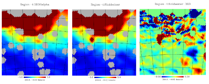
Figure 11: Comparison between the (left) DDD and (centre) F03 H_α templates at 1^∘ resolution, for Region 4 of D06. Right: the difference in structure between the two templates.

Of central importance to this paper, however, is the impact of the observed differences in the templates on our template fits. We have, therefore, performed analyses of a set of 1000 simulations, where we use one template to generate a sky with CMB plus all foregrounds, and then we fit both the correct H_α template and the alternate template to the data. In many regions the cross–correlation coefficients are the same, but in equally many regions systematic differences arise due to even small differences in the templates. In some cases, it is clear where the difference in results likely originates; in region 4 taken from D06 for example, there is an obvious bright spot in the F03 template that is much fainter in the DDD relative to the surrounding structure (see Fig. 11). In other cases, the cause of the difference in results is not apparent among low-level template differences. Moreover, we have found such behaviour not only in regions where the data used in the two H_α templates are different (e.g. VTSS versus SHASSA) but also in regions where the data should be consistent with each other (e.g. the common sky area covered by the SHASSA survey), implying that even relatively small differences in the sky map processing can affect the results in such small regions.

With regards to the data, we find that the mean template fit coefficient to the WMAP K-band data for the 33 regions is $1.01\pm 0.02$ for the DDD template and $8.06\pm 0.05$ for the F03 template (in appropriate units). Indeed, the former results by region are systematically lower than the latter. However, assuming that the F03 results are more correct simply because the results are closer to what we expect (based on idealised properties of the WIM such as an electron temperature of $\sim 8000$ K) is unwise. In the Davies et al. 2006 paper, partly because of the unexpectedly low cross–correlation coefficients, we applied a small additional smoothing to the WHAM regions. This smoothing was an attempt to make up the difference between a $1^{\circ}$ top-hat and a $1^{\circ}$ Gaussian, yet it appears from Fig. 10 that this additional smoothing was not appropriate.

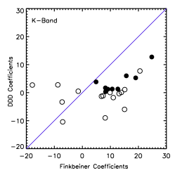
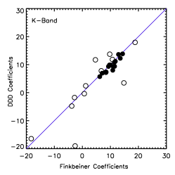
Figure 12: Comparison of the free-free fit coefficients determined between the WMAP K-band data and the DDD and F03 templates at 1^∘ (left panel) and 3^∘ (right panel) resolution.

Nevertheless, it is in smoothing that we find a solution to the issues observed here. After convolving the templates and WMAP data to an effective $3^{\circ}$ resolution, then we find statistically consistent results between the two templates – for example, coefficients of 9.92$\pm$ 0.13 and 10.28$\pm$ 0.13 for the DDD and F03 templates, respectively.

The difference in results between the two templates at $1^{\circ}$ resolution seems to be particularly difficult to reconcile with the power spectrum plots. One would at least expect good agreement in the regions where both templates use only WHAM or SHASSA data. Figs 12 & 13 are therefore quite informative in this respect. It should be clear that the two templates are generally very consistent, although there are more outliers at $1^{\circ}$ resolution. We therefore postulate that it is the nature of the estimator $\alpha=t^{T}M^{-1}d/t^{T}M^{-1}t$ (see Section 3) that amplifies the differences in the templates, as the denominator is sensitive to the square of the template. Though the numerator is roughly the same using both templates, the denominator differs significantly and drives the difference in $\alpha$. At $3^{\circ}$ resolution, the differences are suppressed sufficiently to allow excellent consistency between the results derived with either template.

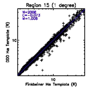
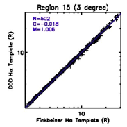
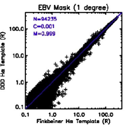
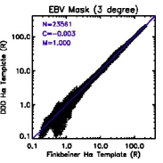
Figure 13: Correlation between the DDD and F03 template maps at 1^∘ and 3^∘ resolution for region 15 (left panels) or the EBV mask (right panels). The thick blue line represents the best fit regression with slope M and intercept C for the number of pixels N. Clearly the scatter of the correlation plot decreases with 3^∘ smoothing.

Though we cannot make a case for the superiority of one template over the other, we choose to utilise the DDD template since it was explicitly constructed to have a uniform resolution over the sky, consistent with the analysis above. Moreover, we wish to emphasise that, in neither case do we consider that the templates are invalid as proxies for the Galactic free-free emission in their higher resolution forms, but that care must be taken as to the properties of the data in local regions. This is particularly important given the subtle interaction between the structure in the data and $\chi^{2}$ type estimators as employed in our analysis.

Appendix B Constructing a regional definition mask

The Davies et al. (2006) regions were selected on the basis that one of the three principal and well-known Galactic foregrounds (free-free, dust or synchrotron emission) was dominant in each region. The regions were selected well away from the Galactic plane where the foregrounds are inevitably confused. In this paper, we extend the analysis by defining regions over a larger fraction of the high latitude sky, and making more extensive use of the template morphology to achieve this. Our approach is also intended to allow a focus on localised areas of the sky where foreground spectral variations may be traced. To achieve this, we recognise that the overall Galactic emission even to high latitudes can generally be well described by a cosecant law of emission (Bennett et al., 2003b), with the possible exception of the 408 MHz emission. Nevertheless, we wish to adopt a uniform processing of the templates. Therefore, by normalising the template emission by a cosecant term, we essentially flatten the structure and enhance local features. We impose a 5^∘ Galactic cut on the templates given that this region will be excluded by our EBV and KQ85 masks in any case, and to avoid the cosecant term causing problems. We then subdivide each template on the basis of intensity, a criterion which, at least in the case of thermal dust emission (Miville-Deschênes et al., 2007), associates variations in the physical properties of the foregrounds with mean brightness. This is then the basis for further processing to select the individual regions. The exact algorithm to define our regions of interest is as follows.

(I)

Consider the three external foreground templates for synchrotron S (408 MHz), free-free F (H_α) and dust D (FDS8) as smoothed to $3^{\circ}$ beam resolution. Denote the emission at a given pixel of component $k$ (S,F,or D) by $T^{k}(\hat{n})$.

(II)

To remove the effect of the line-of-sight depth, we apply a sine modulation to each external template, which is defined as,

$$T^{k}_{\mathrm{sin}}(\hat{n})=\begin{cases}T^{k}(\hat{n})\times\text{sin}\ |b|&\text{if}\quad|b|>5\\ 0&\text{if}\quad|b|<5\end{cases}$$ (12)

where ‘$b$’ represents the Galactic latitude of the given position of the sky defined by $\hat{n}$ , $T^{k}$ and $T^{k}_{\mathrm{sin}}$ represents the external template and the modulated template, respectively. We do not include the $\pm 5^{\circ}$ latitude range above and below the Galactic plane. Each modulated template has a characteristic behaviour which helps to define the morphology of the regions of interest.

(III)

Sort the pixels in each template by temperature such that

$$T_{\mathrm{sin}}^{k}(\hat{n}_{i})<T_{\mathrm{sin}}^{k}(\hat{n}_{i+1})$$ (13)

and then define ten intervals, each with a tenth of the ordered pixels. I.e. for each template, we define the set of pixels

$$\mathbb{S}_{j}^{k}=\{\hat{n}_{i}\}\quad\text{s.t.}\quad 0.1\,N\,(j-1)<i<=0.1\,N\,j$$

$$\qquad\text{where}\quad 1<=j<=10$$ (14)

This effectively divides the sky into ten roughly isotemperature regions of equal total area. We can create a map, $I^{k}(\hat{n})$, of these sets by assigning the pixels the dummy temperature value of $j$ that labels the set, $\mathbb{S}_{j}^{k}$, to which the pixel belongs. These maps are shown in the first row of Fig. 14 for the three templates. Where the map has a value of 10, for example, the pixel in the sine-modulated template map has a temperature in the top 10% of the sky emission.

(IV)

This isotemperature contour map for each template has distinct features and can be used to isolate morphologically interesting regions. We visit each pixel and determine in which template $I^{k}(\hat{n}_{i})$ is maximum and then define a new region map, $R(\hat{n})$ as follows:

$$R(\hat{n}_{i})=a\ \textbf{max}\{I^{k}(\hat{n}_{i})\}$$

$$\qquad\text{where}\quad a=\begin{cases}10&\text{if}\quad\textbf{max}\{I^{k}\}=I^{S}\\ 100&\text{if}\quad\textbf{max}\{I^{k}\}=I^{D}\\ 1000&\text{if}\quad\textbf{max}\{I^{k}\}=I^{F}\end{cases}$$ (15)

This map is shown with various color scalings in the 2nd row of Fig. 14. Levels 10-100 correspond to synchrotron regions, 100-1000 are dust, and 1000-10000 are H_α.

(V)

The new combined map $R(\hat{n})$ has up to ten regions for each template, and these are reduced by a factor of two into 15 (non-contiguous) regions simply by merging regions of similar temperature. This is shown in the left-hand plot of the last row of Fig. 14. Lastly, the discontinuous regions with the same value label are then split, while very small regions are either clumped together or omitted, leaving a total of 35 new regions. The resultant map is shown in lower-right of the figure. Table 7 summarises some useful quantities that describe the regions on the sky.

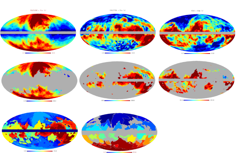
Figure 14: Definition of the new regions as described in § 2.4. Top row: the sine-modulated external synchrotron, free-free and dust templates at $3^{\circ}$ resolution, each rescaled into ten roughly isotemperature regions of equal area. Second row: regions of the sky where where each modulated template is considered morphologically dominant. Last row: the left-hand plot shows the merged map from combining and maps from the middle row. The central plot defines 35 regions constructed from the merged maps. These cover almost the whole sky excluding the $\pm 5^{\circ}$ close to the Galactic plane and some areas where the method resulted in many very small regions that are difficult to merge meaningfully. Note that two of the regions are eventually excluded from analysis when the KQ85 mask is also imposed on the sky.

Region	No. of Pixels (in $N_{side}=64$ map)		Angular Coordinates		Centroid of Region
	Default	Surviving EBV mask	$l$ (in degrees)	$b$ (in degrees)	$l,b$ (in degrees)
1	2047	1877	41∘.5 to 178∘.5	32∘.8 to 88∘.5	(95∘.0, 62∘.2)
2	1611	1433	190∘.7 to 353∘.7	25∘.3 to 87∘.8	(302∘.2, 59∘.2)
3	2825	2508	286∘.9 to 60∘.9	15∘.7 to 88∘.5	(8∘.1, 58∘.3)
4	673	590	180∘.8 to 250∘.1	37∘.9 to 67∘.9	(202∘.1, 55∘.5)
5	168	145	166∘.8 to 179∘.3	35∘.0 to 55∘.9	(174∘.3, 45∘.2)
6	670	585	39∘.4 to 95∘.6	17∘.6 to 52∘.0	(67∘.6, 33∘.2)
7	1624	1507	181∘.4 to 251∘.0	6∘.0 to 56∘.6	(208∘.5, 30∘.4)
8	1026	920	239∘.1 to 333∘.3	8∘.4 to 34∘.2	(287∘.6, 22∘.3)
9	775	260	345∘.9 to 31∘.6	6∘.0 to 41∘.8	(7∘.7, 20∘.9)
10	702	575	128∘.7 to 179∘.3	6∘.0 to 34∘.2	(160∘.4, 18∘.9)
11	696	594	55∘.5 to 111∘.1	6∘.0 to 35∘.0	(75∘.7, 18∘.2)
12	1093	279	79∘.5 to 158∘.9	6∘.0 to 33∘.5	(121∘.0, 14∘.2)
13	421	373	243∘.3 to 277∘.0	6∘.0 to 25∘.3	(260∘.8, 13∘.9)
14	704	551	234∘.1 to 277∘.0	-28∘.6 to -6∘.0	(257∘.5,-14∘.8)
15	598	502	66∘.1 to 99∘.8	-28∘.0 to -6∘.0	(84∘.6,-16∘.6)
16	597	479	9∘.1 to 53∘.4	-30∘.7 to -6∘.0	(31∘.3,-17∘.2)
17	290	269	308∘.7 to 358∘.6	-24∘.0 to -10∘.8	(330∘.2,-18∘.0)
18	627	573	109∘.7 to 149∘.1	-30∘.7 to -9∘.0	(130∘.0,-18∘.9)
19	330	275	229∘.9 to 258∘.7	-30∘.7 to -10∘.2	(238∘.8,-22∘.5)
20	286	135	181∘.4 to 192∘.7	-39∘.5 to -12∘.6	(186∘.2,-26∘.1)
21	899	703	276∘.3 to 319∘.2	-44∘.2 to -10∘.8	(297∘.7,-27∘.5)
22	392	354	87∘.2 to 111∘.1	-41∘.8 to -6∘.0	(101∘.2,-29∘.2)
23	862	496	148∘.4 to 179∘.3	-45∘.8 to -12∘.6	(166∘.8,-28∘.6)
24	918	812	180∘.8 to 228∘.5	-51∘.3 to -12∘.6	(208∘.0,-34∘.4)
25	242	213	54∘.5 to 77∘.9	-49∘.7 to -34∘.2	(66∘.0,-43∘.5)
26	258	231	235∘.2 to 272∘.2	-52∘.0 to -34∘.2	(255∘.2,-44∘.4)
27	395	348	197∘.4 to 239∘.1	-61∘.2 to -30∘.0	(225∘.1,-46∘.7)
28	180	160	87∘.3 to 123∘.9	-55∘.1 to -42∘.6	(106∘.5,-50∘.2)
29	159	144	7∘.9 to 35∘.8	-63∘.4 to -50∘.5	(19∘.8,-56∘.8)
30	195	182	158∘.1 to 179∘.1	-64∘.9 to -48∘.1	(168∘.7,-56∘.9)
31	579	523	181∘.0 to 305∘.2	-67∘.2 to -38∘.7	(250∘.2,-59∘.9)
32	3988	3607	181∘.2 to 148∘.6	-76∘.8 to -18∘.2	(357∘.3,-67∘.5)
33	1507	1363	182∘.6 to 178∘.5	-89∘.3 to -4∘5.0	(109∘.1,-82∘.4)

Table 7: Definition of regions for the template fit analysis. The number of pixels contained in the region by default, and after application of the EBV mask are shown, together with the range of latitude and longitude values spanning a given region, and the angular coordinates of the region centroid.

Appendix C Full Fit Results

Tables 8, 9 & 10 list the solutions for all 33 regions, for the template fit coefficients of the three Galactic foreground components of synchrotron, free-free and dust emission respectively. Discussions of these basic results can be found in Section 4, and model fits to the coefficients are detailed and discussed in Section 5.

	Synchrotron
Region	K	Ka	Q	V	W
EBV	8.53 ±0.20	2.83 ±0.20	1.45 ±0.19	0.42 ±0.19	0.10 ±0.17
KQ85	8.20 ±0.23	2.63 ±0.23	1.32 ±0.23	0.28 ±0.22	-0.02 ±0.19
NPS	5.06 ±0.62	1.48±0.61	0.63 ±0.60	0.08 ±0.58	-0.02 ±0.52
GN	8.73 ±0.28	2.92 ±0.28	1.53 ±0.27	0.49 ±0.26	0.13 ±0.24
GNreduced	9.46 ±0.31	3.26 ±0.30	1.77 ±0.30	0.64 ±0.29	0.22 ±0.26
EN	6.94 ±0.29	2.00 ±0.28	0.82 ±0.28	-0.06 ±0.27	-0.28 ±0.24
ENreduced	7.38 ±0.32	2.19 ±0.31	0.93 ±0.31	-0.01 ±0.30	-0.27 ±0.26
GS	8.39 ±0.29	2.81 ±0.28	1.43 ±0.28	0.36 ±0.27	0.06 ±0.24
ES	8.49 ±0.25	2.96 ±0.25	1.65 ±0.24	0.67 ±0.23	0.35 ±0.21
1	3.7 ±1.9	0.1 ±1.9	-0.5 ±1.8	-0.8 ±1.8	-0.9 ±1.6
2	7.3 ±1.4	2.5 ±1.4	1.1 ±1.4	0.3 ±1.3	-0.1 ±1.2
3	5.0 ±0.6	1.6 ±0.6	0.8 ±0.6	0.3 ±0.5	0.1 ±0.5
4	7.7 ±4.2	4.2 ±4.1	3.4 ±4.0	2.2 ±3.9	2.0 ±3.5
5	5.3 ±6.3	0.1 ±6.2	-0.0 ±6.0	-0.9 ±5.9	-1.8 ±5.3
6	3.7 ±1.7	0.6 ±1.7	-0.1 ±1.7	-0.5 ±1.6	-0.7 ±1.4
7	4.5 ±2.0	0.6 ±2.0	-0.4 ±1.9	-1.0 ±1.9	-1.2 ±1.7
8	9.9 ±0.6	3.2 ±0.6	1.7 ±0.6	0.5 ±0.5	0.1 ±0.5
9	3.1 ±1.3	0.7 ±1.3	0.1 ±1.2	-0.4 ±1.2	-0.6 ±1.1
10	8.4 ±2.5	5.5 ±2.5	5.2 ±2.4	4.6 ±2.3	3.9 ±2.1
11	13.9 ±1.4	3.2 ±1.4	0.8 ±1.4	-0.7 ±1.3	-1.2 ±1.2
12	7.8 ±2.1	3.2 ±2.1	2.2 ±2.0	1.1 ±1.9	0.8 ±1.7
13	2.6 ±1.9	-0.5 ±1.9	-1.1 ±1.9	-1.2 ±1.8	-1.3 ±1.6
14	-2.3 ±2.1	-3.2 ±2.1	-3.0 ±2.1	-2.2 ±2.0	-1.6 ±1.8
15	11.0 ±1.8	2.1 ±1.7	-0.3 ±1.7	-1.8 ±1.6	-2.2 ±1.5
16	6.3 ±0.7	2.1 ±0.7	1.1 ±0.7	0.3 ±0.7	0.1 ±0.6
17	7.2 ±1.4	1.4 ±1.4	0.1 ±1.4	-1.1 ±1.3	-1.1 ±1.2
18	8.5 ±2.2	4.0 ±2.2	3.0 ±2.2	1.7 ±2.1	1.5 ±1.8
19	2.3 ±5.0	-0.2 ±4.9	-0.9 ±4.8	-2.7 ±4.7	-2.3 ±4.2
20	4.9 ±4.2	2.1 ±4.1	2.0 ±4.1	1.1 ±3.9	0.7 ±3.5
21	6.2 ±1.9	1.9 ±1.8	1.0 ±1.8	0.2 ±1.7	-0.0 ±1.5
22	6.1 ±2.7	2.9 ±2.7	2.3 ±2.6	1.6 ±2.5	1.2 ±2.3
23	2.6 ±2.9	-1.2 ±2.8	-2.1 ±2.8	-2.6 ±2.7	-2.7 ±2.4
24	12.8 ±2.5	6.8 ±2.4	5.0 ±2.4	3.5 ±2.3	2.6 ±2.1
25	2.0 ±3.6	-0.3 ±3.5	-0.5 ±3.5	-1.0 ±3.4	-0.9 ±3.0
26	12.0 ±5.7	5.4 ±5.7	3.9 ±5.4	2.9 ±5.3	2.6 ±4.8
27	14.5 ±5.3	7.8 ±5.2	6.3 ±5.1	4.3 ±4.9	3.8 ±4.4
28	2.8 ±6.3	-1.6 ±6.2	-2.6 ±6.1	-4.0 ±5.9	-3.5 ±5.3
29	13.0 ±6.3	7.0 ±6.2	5.7 ±6.1	4.2 ±5.9	3.1 ±5.3
30	2.3 ±5.9	-1.3 ±5.8	-2.1 ±5.7	-2.4 ±5.4	-2.4 ±4.8
31	9.7 ±3.8	0.8 ±3.8	-1.5 ±3.7	-2.8 ±3.6	-2.8 ±3.2
32	7.1 ±1.1	2.4 ±1.1	1.3 ±1.1	0.3 ±1.0	0.2 ±0.9
33	8.9 ±3.1	5.1 ±3.1	4.0 ±3.0	3.1 ±2.9	2.4 ±2.6
Average	6.92 ±0.26	2.11 ±0.26	1.00 ±0.25	0.15 ±0.24	-0.08 ±0.22

Table 8: Template fit coefficients between the WMAP data and the Haslam et al. (1982) 408 MHz data, used as a proxy for Galactic emission due to synchrotron radiation, in units of $\mathrm{\mu K\ K^{-1}_{408~{}MHz}}$. Results are provided for the global regions defined in Section 2.3 and for the 33 sky regions defined in Section 2.4. Monopole and dipole terms are also fitted simultaneously. For the global fits, NPS – North Polar Spur, GN – Galactic North, GN_reduced – Galactic North with the NPS removed, EN – Ecliptic North, EN_reduced – Ecliptic North with the NPS removed, GS – Galactic South, ES – Ecliptic South. The average of the 33 regions is also tabulated for convenience.

	Free-Free
Region	K	Ka	Q	V	W
EBV	9.80 ±0.10	4.78 ±0.09	3.11 ±0.09	1.29 ±0.09	0.48 ±0.08
KQ85	10.43 ±0.20	5.14 ±0.20	3.40 ±0.19	1.45 ±0.19	0.62 ±0.17
NPS	20.99 ±12.11	11.61±11.94	10.35 ±11.74	7.14 ±11.33	5.29 ±10.14
GN	10.31 ±0.18	4.99 ±0.18	3.20 ±0.17	1.16 ±0.17	0.27 ±0.15
GNreduced	10.27 ±0.18	4.97 ±0.18	3.18 ±0.17	1.15 ±0.17	0.26 ±0.15
EN	13.22 ±0.26	6.52 ±0.26	4.32 ±0.25	1.76 ±0.24	0.59 ±0.22
ENreduced	13.12 ±0.26	6.48 ±0.26	4.29 ±0.25	1.75 ±0.24	0.58 ±0.22
GS	9.81 ±0.12	4.79 ±0.12	3.13 ±0.12	1.37 ±0.11	0.57 ±0.10
ES	9.22 ±0.11	4.47 ±0.11	2.89 ±0.10	1.20 ±0.10	0.44 ±0.09
1	-16.4 ±15.6	-15.4 ±15.4	-15.1 ±15.0	-14.9 ±14.7	-13.9 ±13.3
2	11.2 ±5.4	7.2 ±5.3	6.7 ±5.2	4.3 ±5.0	3.3 ±4.4
3	11.8 ±7.7	4.1 ±7.6	2.8 ±7.5	-0.4 ±7.2	-1.4 ±6.5
4	17.9 ±23.8	8.2 ±23.5	3.7 ±23.0	-1.2 ±22.2	-4.3 ±19.9
5	62.3 ±45.0	63.8 ±44.4	65.4 ±43.2	65.0 ±42.3	60.1 ±38.2
6	13.7 ±9.4	9.0 ±9.3	6.6 ±9.0	5.0 ±8.7	4.2 ±7.9
7	9.4 ±2.1	2.7 ±2.1	0.7 ±2.1	-1.4 ±2.1	-2.0 ±1.9
8	6.9 ±1.6	3.8 ±1.5	2.2 ±1.5	0.6 ±1.5	-0.1 ±1.3
9	9.9 ±0.3	5.3 ±0.3	3.7 ±0.3	1.5 ±0.3	0.4 ±0.3
10	-1.8 ±5.5	-4.5 ±5.4	-6.2 ±5.3	-6.5 ±5.2	-5.8 ±4.6
11	25.0 ±0.8	11.1 ±0.8	7.0 ±0.8	3.3 ±0.8	1.9 ±0.7
11 (KQ85)	15.8 ±1.3	7.1 ±1.3	4.4 ±1.3	1.8 ±1.3	1.0 ±1.1
12	9.9 ±2.5	3.3 ±2.4	1.0 ±2.4	-1.3 ±2.3	-1.9 ±2.1
13	9.3 ±0.4	4.3 ±0.4	2.7 ±0.4	1.1 ±0.4	0.4 ±0.3
14	9.8 ±0.2	4.8 ±0.2	3.2 ±0.2	1.4 ±0.2	0.6 ±0.1
15	12.3 ±0.8	6.2 ±0.7	4.3 ±0.7	2.1 ±0.7	1.2 ±0.6
16	7.3 ±5.2	3.8 ±5.1	2.3 ±5.0	0.3 ±4.8	0.2 ±4.3
17	-0.4 ±6.0	0.8 ±5.9	0.7 ±5.8	0.4 ±5.6	-0.3 ±5.0
18	13.8 ±2.0	8.1 ±2.0	5.8 ±2.0	3.6 ±1.9	2.2 ±1.7
19	5.7 ±2.6	2.9 ±2.6	1.4 ±2.5	0.0 ±2.5	-0.4 ±2.2
20	8.0 ±0.9	4.4 ±0.9	3.6 ±0.9	2.2 ±0.9	1.5 ±0.8
21	13.6 ±3.2	8.9 ±3.1	7.6 ±3.0	5.3 ±2.9	3.8 ±2.6
22	7.8 ±5.8	1.6 ±5.7	0.4 ±5.6	-1.5 ±5.4	-2.7 ±4.9
23	10.8 ±1.7	4.7 ±1.6	2.8 ±1.6	0.6 ±1.6	-0.4 ±1.4
24	7.4 ±0.4	3.7 ±0.4	2.4 ±0.4	1.0 ±0.4	0.5 ±0.4
25	2.4 ±13.2	1.2 ±13.0	-1.1 ±12.8	-1.6 ±12.3	-3.1 ±11.0
26	11.7 ±22.5	0.1 ±22.1	-3.4 ±21.3	-8.2 ±20.8	-5.4 ±18.7
27	-4.8 ±6.2	-7.8 ±6.1	-8.5 ±6.0	-9.2 ±5.8	-9.1 ±5.2
28	-25.7 ±44.5	-30.0 ±43.9	-30.8 ±43.0	-30.3 ±41.8	-33.9 ±37.7
29	-42.4 ±23.4	-40.6 ±23.0	-35.0 ±22.6	-35.1 ±22.2	-34.3 ±20.2
30	36.6 ±48.8	27.6 ±48.2	23.3 ±47.2	18.0 ±46.5	10.3 ±42.4
31	-19.0 ±17.4	-27.9 ±17.1	-36.1 ±16.7	-33.0 ±16.1	-27.3 ±14.4
32	9.3 ±3.0	5.9 ±3.0	4.4 ±2.9	3.1 ±2.9	2.4 ±2.6
33	3.5 ±14.9	-1.2 ±14.7	-1.3 ±14.5	-3.0 ±13.9	-3.5 ±12.4
Average	9.92 ±0.13	4.88 ±0.13	3.23 ±0.13	1.42 ±0.12	0.58 ±0.11
(a)	9.54 ±0.13	4.72 ±0.13	3.14 ±0.13	1.37 ±0.12	0.55 ±0.11
(b)	9.60 ±0.13	4.74 ±0.13	3.15 ±0.13	1.38 ±0.12	0.56 ±0.11

Table 9: Template fit coefficients between the WMAP data and DDD H_α data, used as a proxy for Galactic emission due to free-free radiation, in units of $\mathrm{\mu K\ R^{-1}}$. Details as per Table 8. Note that, as described in Section 4.3, region 11 shows evidence of anomalous behaviour in terms of its correlation with the H_α template. We therefore additionally show the corresponding result when the KQ85 mask is imposed instead of the EBV mask. The average of the 33 regions is also tabulated for convenience. (a) is a variant on this in which we completely exclude the region 11 contribution; (b) includes the region 11 (KQ85) values instead of the standard ones.

	Dust
Region	K	Ka	Q	V	W
EBV	9.84 ±0.10	3.80 ±0.10	2.16 ±0.10	1.07 ±0.09	1.24 ±0.08
KQ85	8.23 ±0.09	3.15 ±0.09	1.85 ±0.09	1.06 ±0.08	1.31 ±0.08
NPS	8.58 ±1.57	3.16±1.54	1.75 ±1.52	1.02 ±1.46	1.61 ±1.30
GN	9.61 ±0.16	3.57 ±0.16	1.97 ±0.15	0.97 ±0.15	1.20 ±0.13
GNreduced	9.55 ±0.16	3.55 ±0.16	1.96 ±0.15	0.96 ±0.15	1.20 ±0.13
EN	8.97 ±0.15	3.36 ±0.15	1.88 ±0.15	0.96 ±0.14	1.18 ±0.13
ENreduced	8.85 ±0.15	3.30 ±0.15	1.86 ±0.15	0.95 ±0.14	1.17 ±0.13
GS	10.44 ±0.14	4.14 ±0.14	2.40 ±0.14	1.20 ±0.13	1.29 ±0.12
ES	10.53 ±0.14	4.12 ±0.13	2.34 ±0.13	1.13 ±0.13	1.26 ±0.11
1	10.1 ±3.4	4.2 ±3.4	2.7 ±3.3	1.2 ±3.2	1.6 ±2.9
2	8.8 ±1.8	2.2 ±1.8	0.5 ±1.8	-0.4 ±1.7	-0.2 ±1.5
3	9.5 ±1.1	3.9 ±1.0	2.5 ±1.0	1.9 ±1.0	2.2 ±0.9
4	6.6 ±5.2	3.6 ±5.2	3.2 ±5.1	2.9 ±4.9	3.2 ±4.3
5	5.1 ±9.3	1.9 ±9.1	0.5 ±8.9	0.7 ±8.7	1.4 ±7.8
6	8.1 ±2.6	2.9 ±2.6	1.4 ±2.5	0.7 ±2.4	1.0 ±2.2
7	10.5 ±0.7	4.3 ±0.7	2.6 ±0.7	1.3 ±0.7	1.5 ±0.6
8	7.3 ±0.7	2.8 ±0.7	1.8 ±0.7	1.3 ±0.6	1.5 ±0.6
9	14.0 ±0.5	5.6 ±0.5	3.2 ±0.5	1.5 ±0.5	1.5 ±0.5
10	7.1 ±0.8	2.4 ±0.7	1.2 ±0.7	0.5 ±0.7	0.8 ±0.6
11	4.5 ±0.7	2.1 ±0.7	1.2 ±0.6	0.7 ±0.6	1.0 ±0.6
12	5.8 ±0.4	1.6 ±0.4	0.6 ±0.4	0.1 ±0.4	0.5 ±0.4
13	6.1 ±0.8	2.1 ±0.7	1.1 ±0.7	0.5 ±0.7	0.9 ±0.6
14	10.4 ±0.5	4.3 ±0.5	2.6 ±0.5	1.4 ±0.5	1.5 ±0.4
15	8.9 ±0.6	3.9 ±0.6	2.5 ±0.6	1.7 ±0.6	1.9 ±0.5
16	7.0 ±0.7	1.4 ±0.7	0.2 ±0.7	-0.4 ±0.7	-0.0 ±0.6
17	7.2 ±2.0	2.0 ±2.0	0.5 ±2.0	-0.2 ±1.9	0.4 ±1.7
18	7.6 ±1.0	2.4 ±1.0	1.0 ±1.0	0.4 ±0.9	0.7 ±0.8
19	10.1 ±2.1	5.1 ±2.1	3.9 ±2.1	3.5 ±2.0	3.3 ±1.8
20	10.6 ±0.8	3.9 ±0.8	2.0 ±0.8	0.9 ±0.8	1.1 ±0.7
21	7.5 ±0.5	2.7 ±0.5	1.5 ±0.5	0.8 ±0.4	1.1 ±0.4
22	9.4 ±0.9	4.2 ±0.9	2.6 ±0.9	1.7 ±0.9	2.0 ±0.8
23	9.6 ±0.4	4.0 ±0.4	2.4 ±0.3	1.3 ±0.3	1.4 ±0.3
24	8.4 ±0.6	2.4 ±0.6	0.9 ±0.6	-0.0 ±0.6	0.2 ±0.5
25	4.9 ±2.2	0.4 ±2.1	-0.5 ±2.1	-1.2 ±2.0	-0.9 ±1.8
26	4.4 ±7.1	3.8 ±7.0	3.4 ±6.7	3.6 ±6.7	2.9 ±6.0
27	12.5 ±4.4	6.3 ±4.3	4.8 ±4.2	3.9 ±4.1	3.8 ±3.7
28	9.2 ±2.0	4.4 ±2.0	3.3 ±2.0	2.9 ±1.9	2.8 ±1.7
29	6.3 ±13.4	-1.1 ±13.2	-5.3 ±13.0	-5.3 ±12.6	-5.3 ±11.3
30	10.5 ±3.5	5.0 ±3.5	3.9 ±3.4	2.8 ±3.3	2.8 ±2.9
31	12.9 ±3.6	6.4 ±3.6	4.8 ±3.5	3.5 ±3.4	3.4 ±3.0
32	8.8 ±0.9	3.1 ±0.9	1.9 ±0.9	0.9 ±0.9	1.0 ±0.8
33	9.2 ±2.1	3.3 ±2.0	1.5 ±2.0	0.6 ±1.9	1.0 ±1.7
Average	8.62 ±0.14	3.24 ±0.14	1.81 ±0.14	0.93 ±0.13	1.13 ±0.12

Table 10: Template fit coefficients between the WMAP data and the FDS model 8 data, used as a proxy for Galactic emission due to dust radiative processes, in units of $\mathrm{\mu K\ \mu K^{-1}_{FDS8}}$. Details as per Table 8.

References

- Ali-Haïmoud, Hirata & Dickinson (2009) Ali-Haïmoud Y., Hirata C. M., Dickinson C., 2009, MNRAS, 395, 1055
- Alves et al. (2011) Alves M. I. R., Davies R. D., Dickinson C., Calabretta M., Davis R., Staveley-Smith L., 2011, ArXiv e-prints
- Banday et al. (2003) Banday A. J., Dickinson C., Davies R. D., Davis R. J., Górski K. M., 2003, MNRAS, 345, 897
- Bennett et al. (2003a) Bennett C. L. et al., 2003a, ApJS, 148, 1
- Bennett et al. (2003b) —, 2003b, ApJS, 148, 97
- Bonaldi et al. (2007) Bonaldi A., Ricciardi S., Leach S., Stivoli F., Baccigalupi C., de Zotti G., 2007, MNRAS, 382, 1791
- Brandt & Draine (2011) Brandt T. D., Draine B. T., 2011, ArXiv e-prints
- Copi et al. (2010) Copi C. J., Huterer D., Schwarz D. J., Starkman G. D., 2010, Advances in Astronomy, 2010
- Davies et al. (2006) Davies R. D., Dickinson C., Banday A. J., Jaffe T. R., Górski K. M., Davis R. J., 2006, MNRAS, 370, 1125
- de Oliveira-Costa et al. (2004) de Oliveira-Costa A., Tegmark M., Davies R. D., Gutiérrez C. M., Lasenby A. N., Rebolo R., Watson R. A., 2004, ApJL, 606, L89
- Dennison, Simonetti & Topasna (1998) Dennison B., Simonetti J. H., Topasna G. A., 1998, PASA, 15, 147
- Dickinson, Davies & Davis (2003) Dickinson C., Davies R. D., Davis R. J., 2003, MNRAS, 341, 369
- Dickinson et al. (2009) Dickinson C. et al., 2009, ApJ, 705, 1607
- Dobler, Draine & Finkbeiner (2009) Dobler G., Draine B., Finkbeiner D. P., 2009, ApJ, 699, 1374
- Dobler & Finkbeiner (2008a) Dobler G., Finkbeiner D. P., 2008a, ApJ, 680, 1222
- Dobler & Finkbeiner (2008b) —, 2008b, ApJ, 680, 1235
- Dobler et al. (2010) Dobler G., Finkbeiner D. P., Cholis I., Slatyer T., Weiner N., 2010, ApJ, 717, 825
- Dong & Draine (2011) Dong R., Draine B. T., 2011, ApJ, 727, 35
- Draine & Lazarian (1998a) Draine B. T., Lazarian A., 1998a, ApJL, 494, L19+
- Draine & Lazarian (1998b) —, 1998b, ApJ, 508, 157
- Erickson (1957) Erickson W. C., 1957, ApJ, 126, 480
- Eriksen et al. (2008) Eriksen H. K., Dickinson C., Jewell J. B., Banday A. J., Górski K. M., Lawrence C. R., 2008, ApJL, 672, L87
- Eriksen et al. (2004) Eriksen H. K., Hansen F. K., Banday A. J., Górski K. M., Lilje P. B., 2004, ApJ, 605, 14
- Ferrara & Dettmar (1994) Ferrara A., Dettmar R.-J., 1994, ApJ, 427, 155
- Finkbeiner (2003) Finkbeiner D. P., 2003, ApJS, 146, 407
- Finkbeiner (2004) —, 2004, ApJ, 614, 186
- Finkbeiner, Davis & Schlegel (1999) Finkbeiner D. P., Davis M., Schlegel D. J., 1999, ApJ, 524, 867
- Gaustad et al. (2001) Gaustad J. E., McCullough P. R., Rosing W., Van Buren D., 2001, PASP, 113, 1326
- Giardino et al. (2002) Giardino G., Banday A. J., Górski K. M., Bennett K., Jonas J. L., Tauber J., 2002, AAP, 387, 82
- Gold et al. (2009) Gold B. et al., 2009, ApJS, 180, 265
- Gold et al. (2011) —, 2011, ApJS, 192, 15
- Górski et al. (2005) Górski K. M., Hivon E., Banday A. J., Wandelt B. D., Hansen F. K., Reinecke M., Bartelmann M., 2005, ApJ, 622, 759
- Haffner (1999) Haffner L. M., 1999, PhD thesis, The University of Wisconsin - Madison
- Haffner et al. (2010) Haffner L. M. et al., 2010, in Astronomical Society of the Pacific Conference Series, Vol. 438, Astronomical Society of the Pacific Conference Series, R. Kothes, T. L. Landecker, & A. G. Willis, ed., p. 388
- Hansen et al. (2006) Hansen F. K., Banday A. J., Eriksen H. K., Górski K. M., Lilje P. B., 2006, ApJ, 648, 784
- Haslam et al. (1982) Haslam C. G. T., Salter C. J., Stoffel H., Wilson W. E., 1982, A&AS, 47, 1
- Hoang, Draine & Lazarian (2010) Hoang T., Draine B. T., Lazarian A., 2010, ApJ, 715, 1462
- Hoang, Lazarian & Draine (2011) Hoang T., Lazarian A., Draine B. T., 2011, ArXiv e-prints
- Jarosik et al. (2011) Jarosik N. et al., 2011, ApJS, 192, 14
- King et al. (2010) King O. G. et al., 2010, in Society of Photo-Optical Instrumentation Engineers (SPIE) Conference Series, Vol. 7741, Society of Photo-Optical Instrumentation Engineers (SPIE) Conference Series
- Kogut et al. (1996) Kogut A., Banday A. J., Bennett C. L., Gorski K. M., Hinshaw G., Reach W. T., 1996, ApJ, 460, 1
- Lagache (2003) Lagache G., 2003, AAP, 405, 813
- Lawson et al. (1987) Lawson K. D., Mayer C. J., Osborne J. L., Parkinson M. L., 1987, MNRAS, 225, 307
- Leitch et al. (1997) Leitch E. M., Readhead A. C. S., Pearson T. J., Myers S. T., 1997, ApJL, 486, L23+
- Macellari et al. (2011) Macellari N., Pierpaoli E., Dickinson C., Vaillancourt J. E., 2011, MNRAS, 1674
- Mattila, Juvela & Lehtinen (2007) Mattila K., Juvela M., Lehtinen K., 2007, ApJL, 654, L131
- Miville-Deschênes et al. (2007) Miville-Deschênes M., Lagache G., Boulanger F., Puget J., 2007, AAP, 469, 595
- Paladini, Davies & De Zotti (2004) Paladini R., Davies R. D., De Zotti G., 2004, MNRAS, 347, 237
- Park (2004) Park C.-G., 2004, MNRAS, 349, 313
- Park, Park & Gott (2007) Park C.-G., Park C., Gott, III J. R., 2007, ApJ, 660, 959
- Patanchon et al. (2005) Patanchon G., Cardoso J., Delabrouille J., Vielva P., 2005, MNRAS, 364, 1185
- Peel (2011) Peel, 2011
- Planck Collaboration et al. (2011a) Planck Collaboration et al., 2011a, ArXiv e-prints
- Planck Collaboration et al. (2011b) —, 2011b, ArXiv e-prints
- Planck Collaboration et al. (2011c) —, 2011c, ArXiv e-prints
- Planck Collaboration et al. (2011d) —, 2011d, ArXiv e-prints
- Platania et al. (2003) Platania P., Burigana C., Maino D., Caserini E., Bersanelli M., Cappellini B., Mennella A., 2003, AAP, 410, 847
- Reich & Reich (1988) Reich P., Reich W., 1988, A&AS, 74, 7
- Reynolds et al. (1998) Reynolds R. J., Tufte S. L., Haffner L. M., Jaehnig K., Percival J. W., 1998, PASA, 15, 14
- Schlegel, Finkbeiner & Davis (1998) Schlegel D. J., Finkbeiner D. P., Davis M., 1998, ApJ, 500, 525
- Shaver et al. (1983) Shaver P. A., McGee R. X., Newton L. M., Danks A. C., Pottasch S. R., 1983, MNRAS, 204, 53
- Silsbee, Ali-Haïmoud & Hirata (2011) Silsbee K., Ali-Haïmoud Y., Hirata C. M., 2011, MNRAS, 411, 2750
- Strong, Moskalenko & Ptuskin (2007) Strong A. W., Moskalenko I. V., Ptuskin V. S., 2007, Annual Review of Nuclear and Particle Science, 57, 285
- Strong, Orlando & Jaffe (2011) Strong A. W., Orlando E., Jaffe T. R., 2011, AAP, 534, A54+
- Tauber et al. (2010) Tauber J. A. et al., 2010, AAP, 520, A1
- Witt et al. (2010) Witt A. N., Gold B., Barnes, III F. S., DeRoo C. T., Vijh U. P., Madsen G. J., 2010, ApJ, 724, 1551
- Wood & Reynolds (1999) Wood K., Reynolds R. J., 1999, ApJ, 525, 799
- Ysard, Miville-Deschênes & Verstraete (2010) Ysard N., Miville-Deschênes M. A., Verstraete L., 2010, AAP, 509, L1+