Capture of Irregular Satellites via Binary Planetesimal Exchange Reactions in Migrating Planetary Systems

Abstract

By logging encounters between planetesimals and planets we compute the distribution of encounters in a numerically integrated two planet system that is migrating due to interactions with an exterior planetesimal belt. Capture of an irregular satellite in orbit about a planet through an exchange reaction with a binary planetesimal is only likely when the binary planetesimal undergoes a slow and close encounter with the planet. In our simulations we find that close and slow encounters between planetesimals and a planet primarily occur with the outermost and not innermost planet. Taking care to consider where a planet orbit crossing binary planetesimal would first be tidally disrupted, we estimate the probability of both tidal disruption and irregular satellite capture. We estimate that the probability that the secondary of a binary planetesimal is captured and becomes an irregular satellite about a Neptune mass outer planet is about 1/100 for binaries with masses and separations similar to transneptunian planetesimal binaries. If young exoplanetary debris disks host a binary planetesimal population then outwards migrating outer planets should host captured irregular satellite populations. We discuss interpretation of emission associated with the exoplanet Fomalhaut b in terms of collisional evolution of a captured irregular satellite population that is replenished due to planetary migration.

1 Introduction

The majority of irregular satellites about the gas giant planets in our Solar system are in eccentric and high inclination orbits suggesting that likely originated in heliocentric orbit and were later captured into orbit within a planet’s Hill sphere (see the review by Jewitt & Haghighipour 2007). Irregular satellite populations could have at one time been a source of heavy dust production (Bottke et al., 2010). If irregular satellite populations exist in distant planetary systems then exoplanets could be discovered by detecting scattered stellar light from their associated dust clouds (Kennedy & Wyatt, 2011). The color of the visible light from the detected object, Fomalhaut b, in orbit about the nearby star Fomalhaut, is consistent with that of reflected light from the star (Kalas et al., 2008) and so does not originate from the planet itself but could arise from a planetary ring system (as discussed by Kalas et al. 2008), dust cloud associated with irregular satellites (as proposed by Kennedy & Wyatt 2011) or circumplanetary disk akin to the birth site of the Galilean satellites (e.g., as explored by Canup & Ward 2002).

We focus on extrasolar planets that are in proximity to a debris disk as this disk could host planetesimals that could be captured by the planets in the system, becoming irregular satellites. Neither the Fomalhaut system or the HR8799 system are likely to have strongly scattered or thick planetesimal disks, the Fomalhaut system (Kalas et al., 2005, 2008) because the disk is thin (with disk aspect ratio only $h/r\sim 0.013$ (Quillen et al., 2007), and the HR8799 system (Marois et al., 2010) because the planets are closely spaced and the time until the planet’s cross each others orbits is probably short Gozdziewski & Migaszewski 2009; Fabrycky & Murray-Clay 2010; Moore & Quillen 2011) implying that the planets have not yet experienced close encounters. The Fomalhaut and HR8799 systems can be considered to be analogs to our solar system prior to the late heavy bombardment epoch of our solar system that involved close approaches between the giant planets (the ‘Nice’ model; Tsiganis et al. 2005) and subsequent scattering of the planetesimal disk.

In our Solar system, the irregular satellites were likely captured during planet/planet close approaches during the late heavy bombardment era (Nesvorny et al., 2007). However, the recent discovery of a large transneptunian binary population (Noll et al., 2008) has motivated study of the exchange reaction mechanism for irregular satellite capture (Agnor & Hamilton, 2006; Vokrouhlicky et al., 2008; Philpott et al., 2010; Nogueira et al., 2011). Irregular satellites in orbit around the giant planets prior to the epoch of late-heavy bombardment were likely lost during close approaches between planets (Nesvorny et al., 2007). Little is known about possible irregular satellite populations that could have existed prior to the late heavy bombardment era.

Both exoplanets Fomalhaut b and HR8799 b are located just interior to dusty disks that are generated from collisions of planetesimals and so are called debris disks (Marsh et al., 2005; Su et al., 2009). Planetesimals originating from these disks can be scattered by the outer planet into orbits that cross the orbits of interior planets. The interaction between planetesimals and planets allows the outer planet to migrate outwards into the planetesimal disk via the exchange of angular momentum between planets and planetesimals (Fernandez & Ip, 1984; Ida et al., 2000). As the outermost planet migrates outwards the population of planet crossing planetesimals can be continually replenished.

Kennedy & Wyatt (2011) showed that a dust producing irregular satellite population could be long lived, however they did not explore mechanisms for irregular satellite capture about exoplanets. If the planetesimal disks in these systems contain binary planetesimals, then the exchange reaction mechanism for irregular satellite capture (Agnor & Hamilton, 2006) is a viable mechanism for the capture of irregular satellites about planets from the population of planet-orbit crossing planetesimals. Currently, it is estimated that binaries account for 30% of transneptunian or Kuiper belt objects (KBOs) with inclinations $<5^{\circ}$, and $\sim 5$% of the rest of the KBOs (Noll et al., 2008). If binary planetesimals are common in extrasolar planetesimal disks then the migration of an outer planet into a planetesimal disk would cause binary planetesimals to cross the orbits of giant planets in the system, facilitating the capture of irregular satellites.

A planetesimal binary is disrupted inside the Hill sphere of a planet when the distance to the planet is sufficiently small that the planet’s tidal force overcomes the gravitational attraction of the binary. The disruption can leave an object in a bound orbit around the planet if the velocity of the binary components is sufficiently large and oriented so as to decrease the energy of the lower mass planetesimal when the binary is disrupted (Agnor & Hamilton, 2006; Vokrouhlicky et al., 2008). The probability of irregular satellite capture via binary exchanges depends both on the statistics of close approaches and their energies (Vokrouhlicky et al., 2008; Philpott et al., 2010; Nogueira et al., 2011). In this paper we consider the statistics of close approaches between planetesimals and planets in systems containing two migrating planets. Our goal is to better understand mechanisms for irregular satellite capture that might operate in young exoplanetary systems and prior to the epoch of late heavy bombardment in our Solar system.

2 Close encounter distribution for a migrating two planet system

We numerically study systems containing two planets that are in proximity to a planetesimal disk that is exterior to the two planets. We restrict our study to low eccentricity and low inclination systems. We first discuss our numerical integrations. We compute the distribution of the first close encounter that would disrupt a planetesimal binary. We then consider the velocity distribution of these encounters.

2.1 Numerical Integrations

We have modified the hybrid symplectic integrator QYMSYM (Moore & Quillen, 2011) to record properties of all particles that approach within a Hill radius of a planet. The integrator runs at two levels, an outer level where all particles are integrated with a symplectic integrator with a fixed timestep, $\tau$. When a particle, or particles pass within a planet’s Hill radius the encounter is integrated more carefully with an adaptive stepsize N-body integrator. Here we use the word encounter to denote a trajectory that passes within the Hill radius of a planet, not a collision with a planet. For every particle that passes within a planet’s Hill radius in each larger timestep, $\tau$, we use the adaptive step-size finer integration to record the minimum distance to the planet, and at that location we record the relative energy per unit mass

$$E_{p}={({\bf v-v}_{p})^{2}\over 2}-{GM_{p}\over|{\bf r-r}_{p}|},$$ (1)

where ${\bf v},{\bf v}_{p}$ are the velocities of particle and planet, ${\bf r},{\bf r}_{p}$ are the positions of particle and planet, respectively, and $M_{p}$ is the mass of the planet. For $E_{p}>0$ we compute a velocity

$$V_{\infty}\equiv\sqrt{2E_{p}}$$ (2)

corresponding to the velocity of the particle distant from the planet and with respect to the planet, were the particle and planet isolated and not orbiting the central star. This velocity can be used to estimate the probability that an exchange reaction with a binary planetesimal can occur leaving behind a bound satellite (e.g, Vokrouhlicky et al. 2008) though a more accurate calculation uses the Jacobi constant (Philpott et al., 2010) or directly integrates orbits of all four bodies (Nogueira et al., 2011). Here we do not integrate the four body problem for a planetesimal binary moving in the gravitational field of a planet in orbit about a star. However we do integrate the trajectories of single planetesimals in the gravitational field a planet in orbit about a star and using these trajectories we estimate the probability that a binary would disrupt near the planet.

We work in units of the mass of the central star $M_{*}$, with distance given in units of the initial semi-major axis of the innermost planet, $a_{1}$, and time in units of the initial orbital period of the innermost planet. The masses of the planets are $M_{1},M_{2}$ and semi-major axes $a_{1},a_{2}$. The initial semi-major axes of the planets are $a_{1}=1$ and $a_{2}=1.4$. The initial planet inclinations and eccentricities were set to zero. The initial mean anomaly of the two planets were randomly chosen.

The planetesimal disk properties are identical for all integrations. The initial planetesimal disk is comprised of $N=8192$ objects of mass $m=10^{-7}$ that are distributed between semi-major axes of $a_{min}=1.6$ and $a_{max}=2.5$. The distribution of planetesimal semi-major axes is flat with probability independent of $a$ within $a_{min}$ and $a_{max}$. The initial eccentricity and inclination distributions were chosen using Rayleigh distributions with the mean eccentricity $\bar{e}$ equivalent to twice the mean value of the inclination $\bar{i}$ and $\bar{i}=0.01$. The initial orbital angles (mean anomalies, longitudes of pericenter and longitudes of the ascending node) were randomly chosen. The total mass of the disk is nearly $10^{-3}$ and large enough that the outer planet can migrate a substantial distance through the disk in a few thousand orbits making it feasible to run a number of similar integrations.

Our integrations primarily have inner planet with $M_{1}=10^{-3}$ or $M_{1}=10^{-4}$, however a few were done with intermediate or larger masses. The properties of the numerical integrations are summarized in Table 1. Each simulation was integrated for at least $P=1900$ orbits with orbital periods are measured in units of the inner planet’s initial orbital period. The outer planet migrated outwards in all simulations, however, in some simulations (those with low mass outer planets) the outer planet first migrated outwards and then reversed direction. As a consequence we consider the statistics of encounters only during the portion of the integration when the outer planet migrated outwards. The length of time used to measure properties of encounters is also reported in Table 1 in orbital periods of the innermost planet. Final positions of the planets $a_{1,f}$ and $a_{2,f}$ and the total number of orbit crossing planetesimals, $N_{c}$, are also listed in Table 1. The change in total energy due to numerical integration errors at the end of the integrations was $|\Delta E/E_{0}|\la 10^{-4}$ where $E_{0}$ is the initial energy (see Moore & Quillen 2011 for a discussion about the accuracy of this integrator). The simulations were run using NVIDIA graphics cards from the GT200 architecture (the Quadro FX5800, or the GTX 285) or using Fermi Class Tesla C2050 cards from the GF100 architecture. All of these are capable of computing in double precision.

Table 1: Integrations

$M_{1}$	$M_{2}$	$P$	$a_{1,f}$	$a_{2,f}$	$N_{c}$	$\log_{10}P_{1}$	$\log_{10}P_{2}$
(1)	(2)	(3)	(4)	(5)	(6)	(7)	(8)
$10^{-3}$	$5\times 10^{-5}$	1200	0.99	2.3	5345	-4.43	-1.20
$10^{-3}$	$7\times 10^{-5}$	1500	0.98	2.3	6042	-3.58	-1.26
$10^{-3}$	$10^{-4}$	1910	0.97	2.3	6728	-3.83	-1.31
$10^{-3}$	$3\times 10^{-4}$	1910	0.93	1.9	5234	-3.94	-1.53
$10^{-3}$	$4\times 10^{-4}$	1910	0.92	1.8	4700	-3.53	-1.58
$10^{-3}$	$6\times 10^{-4}$	1910	0.90	1.7	4494	-3.57	-1.66
$10^{-3}$	$7\times 10^{-4}$	1910	0.89	1.7	4738	-3.47	-1.72
$10^{-3}$	$8\times 10^{-4}$	1910	0.88	1.7	5108	-3.33	-1.76
$10^{-3}$	$10^{-3}$	1910	0.88	1.6	4617	-2.87	-1.84
$10^{-4}$	$2\times 10^{-5}$	1400	1.0	2.2	4732	-3.76	-1.36
$10^{-4}$	$3\times 10^{-5}$	1500	1.0	2.2	5310	-3.99	-1.32
$10^{-4}$	$5\times 10^{-5}$	1910	1.0	2.2	3628	-4.12	-1.22
$10^{-4}$	$10^{-4}$	1910	1.0	1.8	3316	-3.78	-1.34
$8\times 10^{-4}$	$8\times 10^{-5}$	1500	0.98	2.3	6031	-3.80	-1.27
$2\times 10^{-3}$	$2\times 10^{-4}$	1910	0.94	2.2	6174	-3.54	-1.47
$3\times 10^{-4}$	$9\times 10^{-5}$	1910	0.98	2.2	5625	-4.06	-1.30
$6\times 10^{-4}$	$9\times 10^{-5}$	1910	0.98	2.3	6182	-3.83	-1.30

This table lists properties of each numerical integration. First and second columns give the masses of the planets in units of the stellar mass; $M_{1}$, $M_{2}$. The time $P$ in orbital periods of the innermost planet (based on its initial orbital period) used to compute statistical properties of encounters are listed in column 3. The semi-major axes of the planets after $P$ orbital periods are listed as $a_{1,f},a_{2,f}$ (columns 4,5). The total number of unique planet orbit crossing planetesimals identified is listed in column 6. Column 7 shows the log of the probability that the inner planet would capture the secondary of a planetesimal binary due to a binary exchange reaction for a binary that disrupts at a normalized tidal disruption radius $R_{td}=0.1$ (as discussed in section 3). This probability is given for planetesimal binary with a primary of radius $s_{1}=100$ km but can be scaled to other planetesimal binaries using factors given in equation 29. The normalized disruption radius, $R_{td}$ is defined in equation 4. Column 8 lists the log of a similar probability but for the outer planet. The probabilities of capture have been estimated from the encounter distributions in the simulations and using equation (29).

Planetesimals originating in the outer disk are first scattered by the outer planet. Afterwards they can cross the orbits of both planets. The interaction between planetesimals and planets allows the outer planet to migrate outwards into the planetesimal disk via the exchange of angular momentum between planets and planetesimals (Fernandez & Ip, 1984). While planetesimals are scattered by planets they can have pericenter near that of a planet’s semi-major axis. On a plot of semi-major axis versus eccentricity these can be seen as scattering surfaces associated with each planet, as seen in previous integrations of planet migration (e.g., Kirsh et al. 2009). To illustrate this, Figure 1 shows the semi-major axis and eccentricity distribution at the end of the integration with $M_{1}=10^{-3}$ and $M_{2}=10^{-4}$. At this time approximately half of the planetesimals have experienced encounters with a planet. The other integrations look similar but with different fractions of particles in each scattering surface and differing numbers of particles in between the planets in orbits that cross the orbits of the two planets.

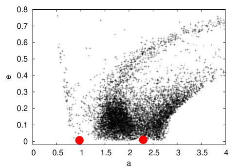
Figure 1: Semi-major axis and eccentricities of particles at the end of the integration with planet masses $M_{1}=10^{-3}$ and $M_{2}=10^{-4}$. Solid circles are the planets. Scattering surfaces are seen for both planets at eccentricities setting pericenters and apocenters near the planets. The outer planet has migrated more than half way through the planetesimal disk.

2.2 Trajectories of planet crossing particles

Because we have logged all particle/planet encounters during the integrations we can examine trajectories of individual particles. In Figure 2 we show an example of the trajectory of a disk particle from the simulation with $M_{1}=10^{-3}$ and $M_{2}=3\times 10^{-4}$ that was ejected near the end of the simulation. We identify ejected particles based on their energies (computed with respect to the central star); those with positive energy have been ejected from the system. In this figure we show the particle’s semi-major axis, $a$, pericenter, $q$, and apocenter, $Q$, as a function of time. We also show simultaneously distance between particle and each planet and the velocity $V_{\infty}$ computed with equation (2) as described above. Encounters are only logged when a particle passes within a Hill radius of a planet so $V_{\infty}$ and $r$ are only plotted during encounters.

When the particle first crosses the orbit of the outer planet it is in a low eccentricity orbit. The velocity of the particle with respect to the planet is not large and so encounters can be gravitationally focused. We see in Figure 2 that a slow and close approach to the outer planet happens before close approaches to the inner planet. The eccentricity of the particle must increase before its orbit can cross those of both planets. The velocity difference between particle and planet is larger when there is a large difference between particle and planet semi-major axis and eccentricity. The inner planet is larger than the outer one in this integration and so the inner planet exchanges more energy with the particle. The trajectory shows a series of distant approaches to the inner planet that slowly increase the energy of the particle. Ejection is not due to a single close encounter with the inner planet. If this particle were a binary planetesimal then it would likely disrupt during one of the slow and close approaches with the outer planet just after it becomes orbit crossing rather than later on when its semi-major axis is high and the relative velocity between planets and particle higher. The trajectory shown in Figure 2 also illustrates that the order of close encounters with the planets is important. A fast but close encounter could disrupt a binary without allowing a capture to take place, hence both the order of encounters and the velocities of disrupting encounters must be taken into account to predict the probability of satellite capture. In the next subsection we compute histograms of disruption locations and velocities during disruption for each planet.

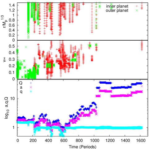
Figure 2: Evolution of a planetary orbit crossing particle. Bottom: We show the log of the semi-major axis (purple crosses), pericenter (light blue stars) and apocenter (dark blue plus signs) as a function of time for a particle that was eventually ejected in the integration with planet masses $M_{1}=10^{-3}$ and $M_{2}=3\times 10^{-4}$. Changes in particle semi-major axes and eccentricity are caused by close encounters with planets. Middle: The velocity with respect to each planet during close encounters. Green points show velocities for encounters with the outer planet and red points show those for the inner planet. We note that early encounters with the outermost planet tend to have the lowest relative velocities. Top: the distance between the object and planet divided by the planet mass to the third power during close encounters. Green points show distances to the outer planet and red points show those to the inner planet. The closest approach at $t\sim 200$ occurs early in the simulation and with the outer planet. This approach also is slow and so could allow the secondary of a binary planetesimal to be captured into orbit about the outer planet during binary disruption. The order of the encounters can be important as an early fast close encounter can disrupt a binary making subsequent irregular satellite capture impossible even if the individual planetesimals later on experience slower encounters.

2.3 Histograms of disruption locations

A planetesimal binary composed of two masses $m_{1},m_{2}$ and separation $a_{B}$ in the vicinity of a planet with mass $M_{p}$ disrupts at a tidal disruption radius

$$r_{td}\sim a_{B}\left({3M_{p}\over m_{1}+m_{2}}\right)^{1/3}$$ (3)

(e.g., Agnor & Hamilton 2006). A planetesimal binary that becomes planet orbit crossing will be disrupted the first time it comes within a tidal disruption radius of a planet. Previous studies have measured distributions of closest approaches in different contexts (Levison & Duncan, 1997; Vokrouhlicky et al., 2008) but have not measured the distribution of disruption radii that depend on both planet mass and the order of close approaches for the idealized migrating system studied here.

A binary disrupts if it passes within its tidal disruption radius of a planet (equation 3). The ratio, $r_{td}/M_{p}^{1/3}$, only depends on binary properties (its separation and total mass). For each encounter that approaches within a radius $r_{td}$ of a planet with mass $M_{p}$ we compute the normalized disruption distance

$$R_{td}={r_{td}\over a_{1,init}}\left({M_{*}\over M_{p}}\right)^{1/3}$$ (4)

where $a_{1,init}$ is the initial semi-major axis of the inner planet. A binary that disrupts at $R_{td}$ has $R_{td}={a_{B}\over a_{1,init}}\left({3M_{*}\over m_{1}+m_{2}}\right)^{1/3}$ only dependent on binary properties. This is why we will measure encounter distances in units of $R_{td}$.

We now consider the range of possible values for $R_{td}$. The planet’s Hill radius is

$$r_{Hp}\equiv a_{p}\left({M_{p}\over 3M_{*}}\right)^{1/3}.$$ (5)

The normalized disruption distance, $R_{td}$, differs from $r_{td}/r_{Hp}$ by a ratio of planet semi-major axes. However since we expect the ratio of planet semi-major axes is of order unity the maximum value of $R_{td}$ is approximately 1. The minimum value of $R_{td}$ occurs when a binary has separation, $a_{B}$, approximately equivalent to the radius of its more massive body. This gives a limit

$$R_{td}\la 10^{-3}\left({\rho\over 1~{}{\rm g~{}cm}^{-3}}\right)^{-{1\over 3}}\left({M_{*}\over M_{\odot}}\right)^{1\over 3}\left({a_{1,init}\over 10~{}{\rm AU}}\right)^{-1}$$ (6)

where $\rho$ is the density of the planetesimals. The range of allowed values for $R_{td}$ sets the range covered by the $x$-axes of our subsequent figures.

For each planet, we count the number of particles that pass within a given disruption radius. At each disruption distance each orbit crossing particle is only counted once. A particle is counted at a disruption distance for the planet that it first approaches within this distance. The result is two histograms (one for each planet) that are functions of $R_{td}$ and that can be used to predict the disruption radius for binaries of a given mass and separation and to predict the planet that is responsible for the disruption. The resulting histograms for simulations with $M_{1}=10^{-3}$ and $M_{2}=\{0.5,1,3,$ and $10\}\times 10^{-4}$ are shown in Figure 3. In these simulations about half of the simulated planetesimals have passed within the Hill radius of a planet. The histograms are normalized by the number of planet orbit crossing particles, $N_{c}$, with this quantity listed for each simulation in Table (1).

Because each particle is only counted one (at each disruption radius) we can determine which planet causes the disruption for each type of binary. Wide and low mass binaries are disrupted at large disruption radii whereas tight and massive binaries disrupted at smaller disruption radii. In Figure 3 we see that wide binaries are most likely to tidally disrupt near the outer planet. For simulations with similar planet masses, tightly bound binaries are more likely to be disrupted by the inner planet. More binaries are disrupted at each disruption radius when the planets are more massive. The difference between the fraction disrupted by the outer planet and that disrupted by the inner planet is largest when the planet mass ratio is large. We expect that an outer planet would have a much richer irregular satellite population than an inner but more massive planet.

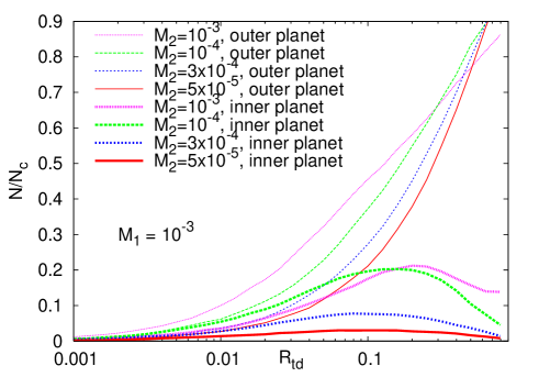
Figure 3: The fraction of orbit crossing particles ($y$-axis) that pass within a disruption distance of $R_{td}$ ($x$-axis) as defined by equation (4) of each planet for four simulations each containing two planets. The properties of the binary (mass and separation) determine the radius at which it would disrupt or $R_{td}$. Four simulations are shown here and all have inner planet with mass $M_{1}=10^{-3}$. The outer planet mass is $M_{2}=0.5,1,3$ or $10\times 10^{-4}$ depending upon the simulation. The top four and thin curves show fractions of particles that approach the outer planets in simulations (from top to bottom) for simulations with $M_{2}=0.5,1,3$ and $10\times 10^{-4}$. The bottom four and thicker curves show fractions for the inner planet for the same simulations. Simulations are labelled by the mass of the outer planet. At each tidal disruption distance, each particle is only counted once and for the planet at which it first approaches within the disruption distance. Weakly bound binaries are preferentially disrupted by the outer planet (high curves on the right hand side of the plot). The difference between the fraction disrupted by the outer planet and disrupted by the inner planet increases as a function of the ratio of inner to outer planet mass.

2.4 Velocity Distributions

During tidal disruption the probability that the secondary of the planetesimal binary is left bound to the planet depends on the incoming velocity of the binary (Agnor & Hamilton, 2006). The secondary is more likely to be captured into orbit if the incoming velocity is low. For 5 different disruption radii we plot in Figure 4 velocity distributions of the disrupting encounters for each of the two planets for the simulation with $M_{1}=10^{-3}$ and $M_{2}=10^{-4}$ (which is also displayed as one of the pairs of curves in Figure 3). The histograms give the fraction of particles with each $V_{\infty}$ value (with $V_{\infty}$ computed using equation 2). These plots have been normalized so that at each disruption radius the sum of the integrated velocity distributions for the two planets is 1. The curves have been smoothed and particles with computed negative $E_{p}$ neglected from the histograms. During encounters some particles have computed negative $E_{p}$ and appear to be bound when they are not because the motion of the planet with respect to the central star has been neglected in the computation of $E_{p}$.

We see in Figure 4 that the velocity distributions differ for each planet with the mean of the distributions significantly higher for the inner planet than the outer planet. Low velocity encounters are much more likely with the outer planet than the inner planet. Tight binaries can be disrupted by the inner planet but have sufficiently high velocities that the capture of the secondary into orbit around the planet is unlikely. The curves associated with the outer planet are higher at zero velocity than those for the inner planet implying that orbit crossing planetesimal binaries are more likely to leave a bound object around the outer planet even if they are more likely to be disrupted by the inner planet. In the next section we estimate the probability of irregular satellite capture based on the low velocity region of these distributions for our different numerical integrations.

Figure 4: Velocity histograms for the simulation with planets $M_{1}=10^{-3}$ and $M_{2}=10^{-4}$ that is also displayed in Figure 3. For 5 different disruption radii ($R_{td}$) we plot the distributions of incoming velocities, $V_{\infty}$, for disrupting close encounters for each planet. The disruption radii are labelled in the key on the upper right. Thick lines correspond to the velocity distributions for the inner planet and thin lines for those of the outer planet. Velocities are in units of the inner planet’s initial circular velocity. The top dotted curve is that for the inner planet and $R_{td}=0.3$ and the bottom solid curve is that for the outer planet and $R_{td}=0.3$. Encounters with the outer planet are more likely to have lower encounter velocities than the inner planet, consequently the outer planet is more likely to capture a secondary during tidal disruption of a planetesimal binary.

As seen from Table 1 for most of our integrations the outer planet migrates a substantial way through the planetesimal disk. By dividing integrations into different time intervals and comparing the distributions based on encounters in these intervals we have checked that the distributions based on the encounters (as shown in Figures 3, 4 and subsequent figures) are not strongly dependent upon time. At the beginning of the integrations the outer planet is near the inner edge of the planetesimal disk. We have found that as long as this edge is sufficiently close to the outer planet to allow migration to take place during the integration, the encounter distributions are insensitive to the disk edge location. We attempted to determine if the distributions were sensitive to disk mass by increasing or decreasing the mass of the planetesimals. However we cannot significantly increase the number of disk particles without increasing the length of computation time. If we significantly decrease the disk or planet masses then planet migration can be extremely slow. Each simulation took a few days to run, consequently we were effectively limited to a narrow region of parameter space in both planet and disk masses. We compromised by fixing the disk mass and then choosing only simulations in which the outer planet migrated a significant distance through the disk.

3 Exchange reactions

We now consider the properties of a planetesimal binary distribution that could lead to capture of an irregular satellite population in a migrating planetary system. We consider a planetesimal binary composed of two masses $m_{1},m_{2}$ and separation, $a_{B}$, in the vicinity of a planet. During tidal disruption in a planet’s tidal gravitational field, the change in velocity of the smaller body, $m_{2}$, due to the orbital speed about the binary’s center of mass

$$\Delta v_{2}\approx{m_{1}\over m_{1}+m_{2}}\sqrt{G(m_{1}+m_{2})\over a_{B}}={m_{1}\over m_{1}+m_{2}}v_{B}$$ (7)

(following Agnor & Hamilton 2006) where the binary internal velocity

$$v_{B}\equiv\sqrt{G(m_{1}+m_{2})\over a_{B}}.$$ (8)

To enable capture, the difference in energy due to the velocity change must exceed the initial energy of the object or $m_{2}V_{\infty}^{2}/2$ where $V_{\infty}$ approximates the velocity (with respect to the planet) before the planet enters the planet’s Hill sphere (equation 2). This condition is easiest to satisfy for the secondary rather than the primary (e.g., Gould & Quillen 2003) hence that is the situation we focus on here.

We define the Hill radius of the binary at its birth semi-major axis $a_{birth}$,

$$r_{HB}\equiv a_{birth}\left({m_{1}+m_{2}\over 3M_{*}}\right)^{1/3}.$$ (9)

The ratio of the tidal disruption radius to the planet’s Hill radius

$${r_{td}\over r_{Hp}}\sim\left({a_{B}\over r_{HB}}\right)\left({a_{birth}\over a_{p}}\right)3^{1/3}$$ (10)

where $a_{p}$ is the semi-major axis of the planet. A binary cannot have a separation larger than its own Hill radius. The above equation implies that the disruption location in units of a planet’s Hill radius primarily depends on the binary separation in units of its own Hill radius. As mentioned in section 2.3, $R_{td}$ differs from $r_{td}/r_{Hp}$ by a factor of planet radii. Thus the normalized disruption radius $R_{td}$ given as the $x$-axis in Figure 3 is approximately the ratio of the binary’s Hill radius to that of the planet. Transneptunian binaries tend to have separations of order $a_{B}/r_{HB}\sim 0.01$ (range 0.002-0.03) (Grundy et al., 2011) and so would disrupt at radius (from the planet) of about 0.01 a giant planet’s Hill radius or with $R_{td}$ of order 0.01.

As the capture probability also depends on the binary’s internal circular velocity, $v_{B}$, (see equation 7) it is useful to consider the maximum and minimum values for this velocity. The binary must be bound so that $a_{B}<r_{HB}$ leading to a minimum binary internal velocity

$${v_{B}\over v_{KB}} \ga 3^{1\over 6}\left(m_{1}+m_{2}\over M_{*}\right)^{1\over 3}$$

$$\ga 10^{-4}\left({s_{1}\over 100{\rm km}}\right)\left({\rho\over 1{\rm g~{}cm}^{-3}}\right)^{1\over 3}\left({M_{*}\over M_{\odot}}\right)^{-{1\over 3}}(1+q_{b})^{1\over 3},$$

where $v_{KB}$ is the Keplerian circular velocity at the binary’s semi-major axis (around the star) and $q_{b}\equiv m_{2}/m_{1}$ is the binary mass ratio. The above is equivalent to requiring $v_{B}>v_{HB}$ where the Hill velocity $v_{HB}=\Omega_{K}r_{HB}$ and $\Omega_{K}$ is the Keplerian angular rotation rate (or mean motion around the star) at the binary’s semi-major axis. When the two planetesimals are nearly touching the binary has a maximum internal velocity of

$${v_{B}\over v_{KB}} \la \sqrt{\rho s_{1}^{2}a\over M_{*}}$$

$$\la 0.003\left({\rho\over 1{\rm g~{}cm}^{-3}}\right)^{1\over 2}\left({M_{*}\over M_{\odot}}\right)^{-{1\over 2}}$$

$$\times\left({a\over 10{\rm AU}}\right)^{1\over 2}\left({s_{1}\over 100{\rm km}}\right).$$

The range of binary internal velocities is restricted by these two limits and is not large. The maximum is larger when the binary in the outskirts of a planetary system as is true for transneptunian binaries.

3.1 Estimating the Probability of Irregular Satellite Capture

In the above section we showed that a binary planetesimal disrupts at a distance from a planet in Hill radii that is primarily dependent on the binary separation in units of its own Hill radius (equation 10). A planetesimal binary could be tidally disrupted but both objects will remain unbound unless the disruption event removes sufficient energy that one of the objects becomes bound to the planet. We now consider the probability that the secondary (from the binary) is captured as a function of the binary’s incoming velocity, $V_{\infty}$, with respect to the planet. We will derive a limit on $V_{\infty}$ that allows a capture to take place. Using this limit we will use our simulations (in which we measure $V_{\infty}$ for close approaches) to estimate the probability that the secondary of a binary planetesimal can be captured into planetary orbit.

The energy per unit mass of a binary approaching a planet

$$E_{0}\approx{V_{\infty}^{2}\over 2},$$ (13)

where we have only taken into account the gravitational field of the planet and neglected that from the star. At the tidal radius, $r_{td}$, the energy per unit mass can be written

$$E_{0}={{\bf v}(r_{td})^{2}\over 2}-{GM_{p}\over r_{td}},$$ (14)

where ${\bf v}(r_{td})$ is the velocity of the orbit at disruption. For the secondary, $m_{2}$, of the binary to become bound to the planet, the change in velocity during disruption must remove sufficient energy that the energy, $E$, becomes negative. The change in energy due to a velocity kick at $r_{td}$ caused by disruption

$$\Delta E={({\bf v}(r_{td})+\Delta{\bf v}_{2})^{2}\over 2}-{v(r_{td})^{2}\over 2}={\bf v}(r_{td})\cdot\Delta{\bf v}_{2}+{(\Delta v_{2})^{2}\over 2}$$ (15)

with $|\Delta v_{2}|$ given by equation (7) and $\Delta E\ga V_{\infty}^{2}/2$ required for capture. Let the angle between the two vectors ${\bf v}(r_{td})$ and $\Delta{\bf v}_{2}$ be $\theta_{v}$. Using the previous equation and this angle, for capture we require that

$$|\Delta v_{2}||v(r_{td})|\cos\theta_{v}+{(\Delta v_{2})^{2}\over 2}\ga{V_{\infty}^{2}\over 2}.$$ (16)

Because the incoming binary is not bound to the planet, the orbital velocity at the moment of tidal disruption, $v(r_{td})$, must always exceed the escape velocity at $r_{td}$. The escape velocity at the tidal disruption radius is

$$v_{escape}(r_{td})=\sqrt{2GM_{p}\over r_{td}}=v_{B}2^{1\over 2}\left({M_{p}\over m_{1}+m_{2}}\right)^{1\over 3}.$$ (17)

We can consider two limits. When the orbit is nearly parabolic, the orbit speed at disruption $v(r_{td})$ is approximately equal to the escape velocity $v(r_{td})=\sqrt{2GM_{p}\over r_{td}}$. If the orbit is highly hyperbolic then $v(r_{td})$ is approximately equal to $V_{\infty}$. The gravitational focusing factor

$$A_{f}=\sqrt{2GM_{p}\over r_{td}V_{\infty}^{2}}={v_{escape}(r_{td})\over V_{\infty}}={v_{B}\over V_{\infty}}2^{1\over 2}\left({M_{p}\over m_{1}+m_{2}}\right)^{1\over 3}$$ (18)

determines the regime; when this factor is low ($A_{f}<1$) the orbit is highly hyperbolic.

It is useful to compare the escape velocity at the tidal disruption radius to the velocity kick $\Delta v_{2}$. Using equations (17) and (7) the ratio

$${v_{escape}(r_{td})\over\Delta v_{2}}=2^{1\over 2}3^{-{1\over 6}}\left({M_{p}\over m_{1}+m_{2}}\right)^{1\over 3}\left({m_{1}+m_{2}\over m_{1}}\right).$$ (19)

Since we expect nearly equal mass binaries the above ratio should exceed 1. As $v_{escape}(r_{td})$ is a lower bound on the orbit velocity at disruption (and $v_{escape}(r_{td}>\Delta v_{2}$) we find that the first term in equation (16) should dominate the second term. Dropping the second term in equation (16) we can approximate the condition for capture as

$$\cos\theta_{v}\ga{V_{\infty}^{2}\over 2v(r_{td})\Delta v_{2}}.$$ (20)

Assuming a random distribution of binary orientations, we can integrate the fraction of the spherical angle that satisfies the above condition (equation 20). We can consider a critical angle, $\theta_{c}$, that is the value of $\theta_{v}$ that gives equality in equation (20). Integrating over solid angle (assuming that all binary orientations equally probable) the probability of capture, $p_{c}$, depends on this critical angle, $\theta_{c}$, with

$$p_{c}\sim{\sin\theta_{c}\over 2}$$ (21)

Using equation (20) the strongly hyperbolic orbit ($A_{f}<1$ and $v(r_{td})\sim V_{\infty}$) gives for capture

$$\cos\theta_{c}\sim{V_{\infty}\over 2\Delta v_{2}}\sim{V_{\infty}\over v_{B}}{m_{1}+m_{2}\over 2m_{1}}.$$ (22)

The nearly parabolic orbit ($A_{f}>1$ and $v(r_{td})\sim v_{escape}(r_{td})$) gives

$$\cos\theta_{c} \sim {V_{\infty}^{2}\over 2v_{escape}(r_{td})\Delta v_{2}}$$ (23)

$$\sim \left({V_{\infty}\over v_{B}}\right)^{2}\left({m_{1}+m_{2}\over 2^{3\over 2}m_{1}}\right)\left({m_{1}+m_{2}\over M_{p}}\right)^{1\over 3}.$$

Note that $\cos\theta_{c}$ is at maximum 1 if the right hand side of either the previous two expressions exceeds 1. Both of these expressions primarily depend on the ratio $V_{\infty}/v_{B}$. Capture is only likely if $\cos\theta_{c}$ is less than 1 and so can only take place if $V_{\infty}/v_{B}$ is small. Since $V_{\infty}/v_{B}$ must be small then $A_{f}\propto v_{B}/V_{\infty}$ must be large (see equation 18) implying that the encounter must be nearly parabolic for capture to take place. This means we can use equation (23) and ignore equation (22). Furthermore the probability drops from 0.5 to 0 over a very small range of values for $V_{\infty}$ and mass ratio $M_{p}/(m_{1}+m_{2})$. We can estimate the condition for capture based on setting the equation (23) to 1 and determining how $V_{\infty}$ depends the properties of the binary at this this dividing line. Setting $\cos\theta_{c}=1$ and inverting equation (23) we find that capture of the secondary during tidal disruption is likely (and has a probability of about 1/2) when

$${V_{\infty}\over v_{B}}\la\left({M_{p}\over m_{1}+m_{2}}\right)^{1\over 6}(1+q_{b})^{-{1\over 2}}2^{3\over 4}$$ (24)

and is nearly zero otherwise. Here the binary mass ratio $q_{b}\equiv m_{2}/m_{1}$. While tidal disruption only depends on radius (from the planet) in units of Hill radii, we see here that the probability of capture also depends on $V_{\infty}/v_{B}$. As more compact and massive binaries have larger orbital velocities they are more likely to leave the secondary as an irregular satellite during a close approach (as previously discussed by Agnor & Hamilton 2006; Philpott et al. 2010). Here we have a quantitative, though approximate condition on $V_{\infty}/v_{B}$ allowing capture which we can use to estimate capture probabilities from the encounter velocity distributions measured in our simulations.

In our integrations we measure velocities in units of the Keplerian rotation velocity (about the star) of the inner planet ($v_{K1}$), hence it is useful to write our condition for capture (equation 24) in terms of $V_{\infty}/v_{K1}$ or

$${V_{\infty}\over v_{K1}}\la\left({M_{p}\over m_{1}+m_{2}}\right)^{1\over 6}\left({(m_{1}+m_{2})\over M_{*}}{a_{1,init}\over a_{B}}\right)^{1\over 2}(1+q_{b})^{-{1\over 2}}2^{3\over 4}$$ (25)

Rather than describe binaries as a function of mass, $m_{1}+m_{2}$, and separation, $a_{B}$, we can describe a binary in terms of its mass and the normalized tidal disruption ratio $R_{td}$ (defined in equation 4). The condition for capture in equation (24) or (25) becomes

$${V_{\infty}\over v_{K1}} \la \left({a_{1,init}\over r_{td}}{M_{p}^{1/3}\over M_{*}^{1/3}}\right)^{{1\over 2}}\left({M_{p}\over M_{*}}\right)^{1\over 6}\left({m_{1}+m_{2}\over M_{*}}\right)^{1\over 6}$$ (27)

$$\times(1+q_{b})^{-{1\over 2}}2^{3\over 4}3^{1\over 6}$$

$$\sim 0.02\left({R_{td}\over 0.1}\right)^{-{1\over 2}}\left({M_{p}/M_{*}\over 10^{-3}}\right)^{1\over 6}\left({\rho\over 1~{}{\rm g~{}cm}^{-3}}\right)^{1\over 6}$$

$$\times\left({s_{1}\over 100~{}{\rm km}}\right)^{1\over 2}\left({M_{*}\over M_{\odot}}\right)^{-{1\over 3}}(1+q_{b})^{-{1\over 3}}.$$

We have estimated that the probability of capture is about 1/2 when the incoming velocity, $V_{\infty}$, is less than the expression we give in equation (27). Our numerically measured distributions of $V_{\infty}$ can now be used to estimate the probability that a distribution of planetesimals will leave behind some captured secondaries. Because only the lowest velocity encounters are relevant we can take the velocity distributions measured from the simulated encounters, shown in Figure 4, and focus on only the number of encounters with incoming velocity near zero. Figure 5 plots the fraction of encounters $N(R_{td})/N_{c}$ passing within a disruption distance that have $V_{\infty}$ within 0 to 0.05 (the value in units of the innermost planet’s Keplerian velocity) for the same simulations shown in Figure 3.

The fraction of encounters with velocities below that given by equation (27) can be estimated by multiplying our numerically measured fraction $N(R_{td})/N_{c}$ integrated over values of $V_{\infty}\in[0,0.05]$ by the factor

$$f={0.02\over 0.05}\left({R_{td}\over 0.1}\right)^{-{1\over 2}}\left({M_{p}/M_{*}\over 10^{-3}}\right)^{1\over 6}.$$ (28)

Here the factor of 0.02, and $R_{td}^{-1/2}M_{p}^{1/6}$ are those in equation (27). We convert this normalized fraction to a probability of irregular satellite capture using an additional factor of 1/2 since the probability of capture is at most 1/2. Thus the probability of a planetesimal capture (based on our numerically measured low velocity fraction of planetary encounters) is

$$P_{cap}(s_{1},R_{td}) \sim 0.2\left.{N(R_{td})\over N_{c}}\right|_{V_{\infty}=0}^{0.05}\left({R_{td}\over 0.1}\right)^{-{1\over 2}}\left({M_{p}/M_{*}\over 10^{-3}}\right)^{1\over 6}$$ (29)

$$\times\left({\rho\over 1~{}{\rm g~{}cm}^{-3}}\right)^{1\over 6}\left({M_{*}\over M_{\odot}}\right)^{-{1\over 3}}$$

$$\times\left({s_{1}\over 100~{}{\rm km}}\right)^{1\over 2}(1+q_{b})^{-{1\over 3}}.$$

To estimate the capture probability we have used a fixed range for $V_{\infty}$ and corrected for the width of this range (rather than integrating to the limit given in equation 27) so that at least a few dozen particles are counted at low $V_{\infty}$ for all planets in all integrations. As the velocity distribution decreases with increasing $V_{\infty}$ for the outer planet and vice versa for the inner planet (see Figure 4) we have somewhat (but not significantly) underestimated the capture probability for the inner planet and overestimated it for the inner planet.

We show in Figure 6 the probability of capture of the secondary by each planet, for a primary planetesimal radius $s_{1}=100$ km and low binary mass ratio, $q_{b}$, and for the same simulations shown in Figure 3 and 5. For other values of stellar mass, $M_{*}$, planetesimal density, $\rho$, binary mass ratio, $q_{b}$, and planetesimal primary radius, $s_{1}$, the probability can be adjusted using scaling given in equation (29).

A comparison between Figures 5 and 6 shows that the probability of capture is reduced from that computed with a fixed velocity range for more weakly bound binaries (larger $R_{td}$). This follows as more weakly bound binaries have lower internal rotational velocities and so cannot exchange as much kinetic energy during disruption as more tightly bound binaries. We see from Figure 6 that the probability of capture about the outer planet is only weakly dependent on the mass of the outer planet. However, the contrast between the capture probability for the outer and inner planet is higher when the planet mass ratio is larger. When the ratio of the planet masses $M_{2}/M_{1}$ is low, the capture probability for weakly bound binaries (large $R_{td}$) is higher than for $M_{2}/M_{1}\sim 1$. This is counter-intuitive as it suggests that additional weakly bound binaries are captured by the inner planet when the outer planet is more massive. The probability of capture by the outer planet is remarkably insensitive to the ratio of the planet masses. However it would be non-trivial to predict the shape of these probability curves and how they depend on planet masses and ratios.

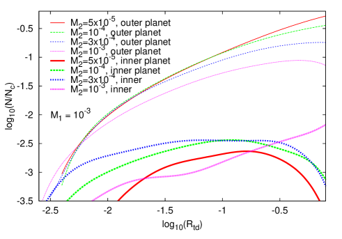
Figure 5: Fraction of integrated particles with incoming velocity $V_{\infty}$ between 0 and 0.05 (in units of the inner planet’s Keplerian velocity) for the integrations shown in Figure 3 as a function of different normalized binary disruption radii, $R_{td}$. The curves have been normalized by the number of orbit crossing particles in the simulation, $N_{c}$. Thick lines correspond to the encounters with inner planets and thin lines to those with the outer planets. In all cases slow encounters are more likely with the outer planet and so this planet is more likely than the inner planet to capture satellites through binary planetesimal exchange reactions.

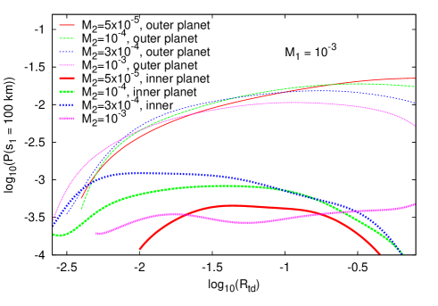
Figure 6: The probability that a binary with primary radius $s_{1}=100$ km would leave its secondary captured as a function of normalized tidal disruption radius, $R_{td}$, for the integrations shown in Figures 3 and 5. Using equation (29) the capture probably can be adjusted for different binary planetesimal masses, mass ratios and densities. The probabilities have been calculated from the fraction of integrated planetesimals approaching planets at low velocities and using factors given in equation (28). Thick lines correspond to probabilities for the inner planets and thin lines to those for the outer planets. In all cases the outer planet is more likely to capture satellites than the inner planet. The probability that the outer planet captures a 100 km radius planetesimal from a binary with a tidal disruption radius $r_{td}/r_{Hp}$ in the range 0.01 to 0.1 is about 1/100.

Our estimated capture probability $\sim 1\%$ is consistent with that estimated by Nogueira et al. (2011) for the capture of Triton via binary exchange reactions during Neptune’s slow migration outwards following close encounters by the giant planets within the context of the “Nice” model. But as shown here only the outermost planet would tend to capture satellites during this slow period of migration, so other scenarios are required to account for the similarity of the irregular satellite populations of the giant planets (Jewitt & Haghighipour, 2007) and so the majority of irregular satellites in our Solar system.

If dust associated with a satellite population is detected in the vicinity of an outer exoplanet but there is no inner planet detected, then it would be helpful if the ratio of satellite capture probabilies could be used to place limits on the planet masses. In Figure 7 using different simulations we plot the ratio of the capture probability for the outer planet and that of the inner planet as a function of the outer planet’s mass. The capture probabilities are those at a disruption radius $R_{td}=0.1$ and for primary planetesimal radius $s_{1}=100~{}$km and are listed for the different simulations in Table 1. Figure 7 shows that the difference in capture probabilities is sensitive to the outer planet mass with lower mass outer planets preferentially capturing more bodies. However, the ratio of capture probabilities appears to be fairly insensitive to the inner planet mass. We note that the two planet masses were necessarily constrained to be in a narrow range because of numerical limitations (we did not want to integrate more than a few thousand orbits). More diverse and challenging simulations would be needed to determine if constraints on planet masses could be based on captured satellite populations. For the range covered by our simulations the ratio is about two orders of magnitude suggesting that outer planets would preferentially be detected from dust associated with an irregular satellite population.

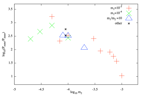
Figure 7: The ratio of the satellite capture probability of the outer planet divided by that of the inner planet ($y$-axis) is shown as a function of outer planet mass ($x$-axis) on a log scale. Points for each simulation are taken from Table 1. For most situations the ratio of capture probabilities is two orders of magnitude suggesting that outer planets would preferentially be detected from dust associated with an irregular satellite population.

4 Collisional evolution of a population of captured irregular satellites

Planetesimals captured into planetary orbit contribute to a dust producing collisional cascade if they collide with other irregular satellites or other objects passing within the Hill radius of the planet. Kennedy & Wyatt (2011) primarily considered the evolution of a primordial irregular satellite population. However if a planet migrates outwards then the irregular satellite population can be replenished by recently captured satellites. The proximity of Fomalhaut’s dust disk to Fomalhaut b suggests that this planet could be migrating outwards. If so the planetesimal disk can provide a continuing source of irregular captured satellites around Fomalhaut b. The rate that irregular satellites are captured can be described as a mass rate, $\dot{M}_{s}$, the mass in irregular satellites captured per unit time. The total rate is integrated over the planetesimal distribution, however because the planetesimal mass distribution is likely dominated by the most massive objects it is simpler to approximate the rate by only considering the massive binary population;

$$\dot{M}_{s}\sim\dot{m}_{o}f_{B}q_{typ}P_{typ}$$ (30)

where $f_{B}$ is the fraction of mass in massive binaries with typical separations, $a_{B,typ}$, mass ratios, $q_{typ}$, and typical total mass, $m_{typ}$. Here $P_{typ}$ is the probability that a binary with these properties would be disrupted and leave a bound satellite around the outer planet. The mass rate $\dot{m}_{o}$ is the mass of planetesimals from the disk that is launched per unit time into orbits that cross the planets. This rate is determined by the migration rate of the outer planet or

$$\dot{m}_{o}=2\pi a_{p}\Sigma_{d}\dot{a}_{p}\sim M_{disk}{a_{p}\over w_{disk}}{\dot{a}_{p}\over a_{p}}$$ (31)

where $a_{p}$ is the semi-major axis of the outer planet that is migrating at a rate $\dot{a}_{p}$ into a planetesimal disk of surface density $\Sigma_{d}$. The planetesimal disk has mass $M_{disk}\sim 2\pi a_{p}w_{disk}\Sigma_{d}$ where $w_{disk}$ is the width of the planetesimal belt. In the case of a single planet embedded in a disk (Ida et al., 2000; Kirsh et al., 2009), when there is adequate disk material to maintain migration then the migration rate is independent of the planet mass with

$${\dot{a}_{p,single}P\over a_{p}}\approx{4\pi\Sigma a_{p}^{2}\over M_{*}}\sim 2{M_{disk}\over M_{*}}{a_{p}\over w_{disk}}$$ (32)

where $P$ is the orbital period of the planet. We can describe planet migration rates in terms of this fiducial value and using a unitless parameter $\eta_{mig}$ with $\dot{a}_{p}\equiv\eta_{mig}\dot{a}_{p,single}$. For comparison, in our integrations the outer planets have migration rates ranging from $\eta_{mig}\sim$ 0.2 – 1.5.

Combining equations (30, 31, 32) we find

$${\dot{M}_{s}P\over M_{p}} \sim \left(M_{disk}\over M_{p}\right)^{2}\left(a_{p}\over w_{disk}\right)^{2}\left(M_{p}\over M_{*}\right)2\eta_{mig}q_{typ}f_{B}P_{typ}$$

$$\sim 10^{-6}\left({M_{disk}/M_{p}\over 0.1}\right)^{2}\left({w_{disk}/a_{p}\over 0.2}\right)^{-2}$$

$$\times\left({M_{p}/M_{*}\over 10^{-3}}\right)\eta_{mig}q_{typ}\left({f_{B}\over 0.3}\right)\left({P_{typ}\over 0.01}\right).$$

where we have chosen the fraction of mass in binaries, $f_{B}$, appropriate for the low inclination transneptunian objects (Noll et al., 2008). Because the capture probability depends on the binary velocity (that has only a narrow range) low mass objects are unlikely to be captured. The above mass rate then represents few and rare events occurring over a moderate time period. As discussed by previous studies (Estrada & Mosqueira, 2006; Philpott et al., 2010; Bottke et al., 2010) a system with only a few irregular satellites could still experience significant collisional evolution.

We can consider a steady state where the captured massive irregular satellites drive a collisional cascade in the vicinity of the planet with a dust production and mass loss rate $\dot{M}_{d}$ equivalent to the rate that mass is gained into the planet’s Hill radius via capture of satellites; $\dot{M}_{d}=\dot{M}_{s}$.

The dust production rate can be estimated from the opacity of the small dust particles in the system, $\tau_{d}$ with radius $s_{d}\sim 10\mu$m. Smaller dust particles are removed from the system due to radiation pressure or PR drag (see discussion by Kennedy & Wyatt 2011). The rate of collisions is $\sim\tau_{d}\Omega$ and so the dust production rate

$$\dot{M}_{d}\sim\rho_{d}s_{d}r_{c}^{2}\tau_{d}^{2}\Omega(r_{c})$$ (34)

where $r_{c}$ the radius of the dust cloud and the dust has density $\rho_{d}$. The luminosity of the dust cloud in units of the stellar luminosity depends on the opacity and size of the cloud

$${L_{d}\over L_{*}}\sim{\tau_{d}r_{c}^{2}Q_{a}\over 4a_{p}^{2}}$$ (35)

where $Q_{a}$ is the albedo. The luminosity ratio is an observable quantity and so relevant for the discussion of emission from Fomalhaut b.

Inside the Hill radius of a planet we can describe radii in units of the Hill radius $\xi\equiv r/r_{H}$. The angular rotation rate $\Omega(r)/\Omega_{K}=\xi^{-3/2}$ where $\Omega_{K}$ is that of the planet in orbit about the star. We define $\xi_{c}\equiv r_{c}/r_{H}$ as the irregular satellite cloud radius in units of the planet’s Hill radius. The luminosity ratio and dust production rate can be written

$$\dot{M}_{d} \sim \rho_{d}s_{d}\tau_{d}^{2}\xi_{c}^{1/2}\mu^{2/3}a_{p}^{2}\Omega_{K}$$

$$\sim 3\times 10^{-4}{M_{\oplus}\over{\rm Myr}}\left({\xi_{c}\over 0.2}\right)^{{1\over 2}}\left({M_{p}/M_{*}\over 10^{-3}}\right)^{{2\over 3}}\left({\tau_{d}\over 0.01}\right)^{2}$$

$$\times\left({\rho_{d}\over 1{\rm g~{}cm}^{-3}}\right)\left({s_{d}\over 10\mu{\rm m}}\right)\left({a_{p}\over 10AU}\right)^{1\over 2}\left({M_{*}\over M_{\odot}}\right)^{1\over 2}$$

where $\mu=M_{p}/M_{*}$ and

$${L_{d}\over L_{*}} \sim {\tau_{d}\xi_{c}^{2}\mu^{2/3}Q_{a}\over 4\times 3^{2/3}}$$

$$\sim 5\times 10^{-8}\left({\tau_{d}\over 0.01}\right)\left({\xi_{c}\over 0.2}\right)^{{2}}\left({M_{p}/M_{*}\over 10^{-3}}\right)^{{2\over 3}}\left({Q_{a}\over 0.1}\right).$$

Here we have chosen parameters ($\tau_{d},Q_{a},\xi_{c},M_{p}$) based on previous scenarios that account for Fomalhaut b’s emission (Kalas et al., 2008; Kennedy & Wyatt, 2011).

So as to compare to a planet migration rate we show the dust production rate in units of the planet’s mass and orbital period, $P$,

$${\dot{M}_{d}\over M_{p}P^{-1}} \sim 2\pi\rho_{d}s_{d}\tau_{d}^{2}\xi_{c}^{1/2}\mu^{2/3}a_{p}^{2}M_{p}^{-1}$$

$$\sim 3\times 10^{-9}\left({\xi_{c}\over 0.2}\right)^{{1\over 2}}\left({M_{p}/M_{*}\over 10^{-3}}\right)^{-{1\over 3}}\left({\tau_{d}\over 0.01}\right)^{2}$$

$$\left({\rho_{d}\over 1{\rm g~{}cm}^{-3}}\right)\left({s_{d}\over 10\mu{\rm m}}\right)\left({a_{p}\over 100AU}\right)^{2}\left({M_{*}\over M_{\odot}}\right)^{-{2\over 3}}.$$

We can compare the rate that mass is captured into planetary orbit (equation 4) with the dust production rate (equation 4). The above extremely modest dust production rate is below the mass that could be captured in irregular satellites. A collisional cascade could be maintained if even a small fraction of orbit crossing planetesimals are captured into an irregular satellite population as the outer planet migrates outwards. If the collision rate and opacity becomes high then small objects could be re-accreted onto larger ones. At a sufficiently high opacity a dense and thin ring system could form.

As discussed by Kennedy & Wyatt (2011) there is only a small range of parameter space for possible irregular satellite clouds that could account for the optical emission in the vicinity of Fomalhaut b. Here we find that this constraint might relaxed if the cloud is replenished by incoming captured satellites. These would have to be fairly massive (and so rare) to be captured, however their lifetime depends not only the timescale that they collide with other object bound objects but also with the time it takes them to collide with the population of orbit crossing planetesimals (including planetesimals that are not binaries). As the planet migrates outwards the irregular satellite population would build up until there is a balance between mass acquired by the system (in the form of captured objects that are then fragmented by collisions with either each other or external objects) and mass lost that is either removed from the system by radiation forces, or accreted back onto other objects. If the opacity is sufficiently high then debris could coalesce into a ring.

5 Discussion and Summary

Using numerical integrations of planets interacting with a planetesimal belt we have explored the statistics of close encounters of planetesimals with planets during planetary migration. We have focused exclusively on the problem of a two planet system in proximity to a cold (in terms of velocity dispersion) planetesimal belt exterior to both planets that induces planetary migration. If the planetesimal belt contains binary planetesimals then close encounters with planets can disrupt these binaries. To predict the location of tidal disruption (at what radius and which planet), we have taken into account the order of close encounters with planets. We find that the velocity distribution (for velocities with respect to the planet) of tidally disrupting encounters differs for the two planets. Lower velocity encounters are only likely with the outer planet. As a consequence we predict that the probability that irregular satellites are captured due to binary exchange reactions is higher, by about two orders of magnitude, with an outer planet than an inner one. We estimate that planetesimal binaries similar to those in the Kuiper belt would have a probability of about 1/100 of disrupting and leaving a bound object about an outer migrating planet. Our numerical estimate is consistent with that recently estimated by Nogueira et al. (2011) for the capture of Triton into orbit about Neptune. In migrating systems we infer that only the outer planet could gain a significant population of captured irregular satellites and other scenarios would be needed to account for irregular satellite populations around inner giant planets. We note that the simulations considered here were restricted by numerical considerations to a narrow range of planet and disk masses, only considered cold and exterior planetesimal disks, only considered two giant planet systems and situations lacking planetary encounters. Future studies can expand the types of systems numerically integrated to predict the probability of satellite capture for more diverse systems.

We estimate that the tidal disruption radius in units of the planet’s Hill radius is approximately set by the binary separation in units of its own Hill radius. Thus if optical emission from exoplanets is associated with a dust cloud generated by irregular satellites, as explored by Kennedy & Wyatt (2011), then there is a relation between the size of the dust cloud, the planet mass and the properties of the primordial binary planetesimal population. We estimate that capture is allowed only if the incoming binary velocity, with respect to the planet is only a few times the velocity of the binary orbit prior to disruption. We have used this estimate and our numerically measured encounter distributions to estimate the probability that the secondary of a binary planetesimal could be captured into orbit about a planet. To improve upon our derived capture probabilities it is likely that the four body problem (binary planetesimal encounter with a planet in orbit about a star) must be integrated.

Kennedy & Wyatt (2011) suggested that irregular satellites can be captured if Fomalhaut b crosses into the planetesimal belt. Here we explore a related scenario. We consider Fomalhaut b not crossing into the planetesimal belt, but migrating outwards and capturing planetesimals due to binary exchange reactions with binaries that have been perturbed into planet orbit crossing trajectories. A crude estimate of the mass in irregular satellites captured per unit time suggests that the mass captured per unit time could be larger than the estimated dust production rate if a collisional cascade operates among the irregular satellite population. Consequently there could be sufficient mass captured as irregular satellites to fuel such a collisional cascade. In a migration scenario, we find that the outer planet is likely to gain two orders of magnitude more irregular satellites than inner planets. It is tempting to consider this scenario as accounting for the detection of Fomalhaut b but not other, possibly more massive planets that could exist interior to it in the system (Kenworthy et al., 2009). Further study is needed to determine whether a migration scenario for Fomalhaut b that included irregular satellite capture would be consistent with the $\sim 0.1$ eccentricity of the dust ring and planet and the location and shape of the ring edge.

Acknowledgements. This work was in part supported by NSF through award AST-0907841. We thank NVIDIA for gift of graphics cards. We thank Scott Gaudi for interesting comments.

References

- Agnor & Hamilton (2006) Agnor, C. B. & Hamilton, D. P. 2006, Nature, 441, 192
- Bottke et al. (2010) Bottke, W. F., Nesvorny, D., Vokrouhlicky, D., & Morbidelli, A. 2010, AJ, 139, 994
- Canup & Ward (2002) Canup, R. M.. & Ward, W. R. 2002, AJ, 124, 3404
- Estrada & Mosqueira (2006) Estrada, P. R., & Mosqueira, I. 2006, Icarus, 181, 496
- Fabrycky & Murray-Clay (2010) Fabrycky, D. C., & Murray-Clay, R. A. 2010, ApJ, 710, 1408
- Fernandez & Ip (1984) Fernandez, J. A., & Ip, W.-H. 1984 , Icarus, 58, 109
- Gozdziewski & Migaszewski (2009) Gozdziewski, K., & Migaszewski, C. 2009, MNRAS, 397, 16
- Grundy et al. (2011) Grundy, W. M., Noll, K. S., Nimmo, F., Roe, H. G., Buie, M. W., Porter, S. B., Benecchi, S. D., Stephens, D. C., Levison, H. F., & Stansberry, J. A. 2011, Icarus, 213, 678
- Gould & Quillen (2003) Gould, A., & Quillen, A. C. 2003, ApJ, 592, 935
- Ida et al. (2000) Ida, S., Bryden, G., Lin, D.N.C., & Tanaka, H., 2000, ApJ, 534, 428
- Jewitt & Haghighipour (2007) Jewitt, D., & Haghighipour, N. 2007, Annu. Rev. Astron. Astrophys., 45, 261
- Kalas et al. (2005) Kalas, P., Graham, J. R. & Clampin, M. 2005, Nature 435, 1067
- Kalas et al. (2008) Kalas, P. et al. 2008, Science, 322, 1345
- Kennedy & Wyatt (2011) Kennedy, G. M., & Wyatt, M. C. 2011, MNRAS, 412, 2137
- Kenworthy et al. (2009) Kenworthy, M. A., Mamajek, E. E., Hinz, P. M., Meyer, M. R., Heinze, A. N., Miller, D. L., Sivanandam, S., & Freed, M. 2009, ApJ, 697, 1928
- Kirsh et al. (2009) Kirsh, D.R., Duncan, M., Brasser, R., & Levison, H.F. 2009, Icarus, 199, 197
- Levison & Duncan (1997) Levison, H. L., & Duncan, M. J. 1997, Icarus, 127, 13
- Marsh et al. (2005) Marsh, K. A., Velusamy, T., Dowell, C. D., Grogan, K., & Beichman, C. A. 2005ApJ…620L..47M
- Marois et al. (2010) Marois, C., Zuckerman, B., Konopacky, Q. M., MacIntosh, B., & Barman, T. 2010, Nature, 468, 7327, 1080
- Moore & Quillen (2011) Moore, A., & Quillen, A. C. 2011, New Astronomy, 16, 445
- Nesvorny et al. (2007) Nesvorny, D., Vokrouhlicky, D., & Morbidelli, A. 2007, ApJ, 133, 1962
- Noll et al. (2008) Noll, K.S., Grundy, W.M., Stephens, D.C., Levison, H.F., Kern, S.D., 2008, Icarus, 194, 758
- Nogueira et al. (2011) Nogueira, E., Brasser, R., & Gomes, R. 2011, Icarus, 214, 113
- Philpott et al. (2010) Philpott, C. M., Hamilton, D. P., & Agnor, C. B. 2010, Icarus, 208, 824
- Quillen et al. (2007) Quillen, A. C., Morbidelli, A., & Moore, A. 2007, MNRAS, 380, 1642
- Su et al. (2009) Su, K. Y. L., Rieke, G. H., Stapelfeldt, K. R., Malhotra, R., Bryden, G., Smith, P. S., Misselt, K. A., Moro-Martin, A., & Williams, J. P. 2009, ApJ, 705, 314
- Tsiganis et al. (2005) Tsiganis, K., Gomes, R., Morbidelli, A., & Levison, H. F. 2005, Nature, 435, 459
- Vokrouhlicky et al. (2008) Vokrouhlicky, D., Nesvorny, D. & and Levison, H. F. 2008, AJ, 136, 1463