Creating atom-number states around tapered optical fibres by loading from an optical lattice

Abstract

We describe theoretically a setup in which a tapered optical nanofibre is introduced into an optical lattice potential for cold atoms. Firstly, we consider the disturbance to the geometry of the lattice potential due to scattering of the lattice lasers from the dielectric fibre surface and show that the resulting distortion to the lattice can be minimized by placing the fibre at an appropriate position in the lattice. We then calculate the modifications of the local potentials that are achievable by transmitting off-resonant light through the fibre. The availability of such a technique holds the potential to deterministically create and address small well-defined samples of atoms in the evanescent field of the tapered nanofibre.

I Introduction

During the last two decades, advances in the cooling and trapping of atoms and ions has assisted in the creation of clean and highly controllable systems, in which fundamental quantum mechanical experiments can be carried out with very low levels of noise. This has led to several breakthrough successes in the quest for implementing ideas of quantum information processing (QIP) Stolze:08 , high-precision atomic clocks Wilpers:04 and quantum metrology Ye:08 .

For neutral atoms optical lattices have been important and hold a great deal of promise in this area. The high degree of control one has over the laser parameters has allowed for the execution of many seminal experiments in these periodic systems. In particular, by controlling the amplitude of the lasers one can adjust the trapping depth, which can act as a switch between regimes in which the dynamics are controlled either by tunnelling between different lattice sites or by interactions between the atoms. This has led to the celebrated observation of the superfluid-Mott insulator transition, in which a state with one atom per lattice site can be created Jaksch:98 ; Greiner:02 .

States which have a well-defined number of particles, so-called atomic Fock states, are currently of large interest in physics. Their sub-Poissonian number statistics is valuable for applications in atom-metrology, quantum information processing and has merit for investigating the foundation of quantum mechanics as well. Several ground-breaking experiments have recently reported the creation of such states Chuu:05 ; Esteve:08 ; Itah:10 and a significant amount of theoretical work has been devoted to their characterization Sokolovski:11 ; Pons:11 . Knowing the exact number of atoms a priori in each run of the experiment is still a difficult task, and techniques which can deterministically create a desired atom number are under vigorous development.

Here we present a near-field optics approach to creating such definite atom-number states and propose the use of the evanescent field of an optical fibre as a tool for manipulating the optical lattice potential locally (see Fig. 1). While standard optical fibres have a diameter of several hundred $\mu$m, recent progress in tapering techniques allows for the creation of fibres of subwavelength diameter Morrissey:09 and even down to 50 nmTong:03 . A significant amount of the intensity in these fibres is carried in their evanescent field and can therefore be used to create an optical potential for ultracold atoms. In this work we will examine the effects of introducing a sub-micrometer fibre into an optical lattice and demonstrate the possibility of deterministically creating states of fixed particle number using appropriately chosen fields inside the fibre.

The paper is organized as follows: in Sec. II we will present a short review of the potential forces relating to optical lattices and sub-micrometer diameter, single-mode silica fibres. We then discuss the modifications of an optical lattice potential due to effects from light scattering on a fibre in Sec. III and examine several achievable potential geometries resulting from the combination of the lattice potential and the evanescent field potentials in Sec. IV. The resulting atomic state is discussed in Sec. V and we finally conclude in Sec. VI.

II Potential Forces

II.1 Optical Lattices

To understand the influence the introduction of the fibre into an optical lattice has, let us first briefly review the optical potentials associated with optical lattices and nano-fibres. Optical lattices exist by today in many laboratories and represent periodic arrays of micro-traps generated by the dipole force of a standing wave laser light field Jaksch:98 ; Greiner:02 ; Bloch:08 . A variety of trapping geometries are achievable, with the most common being rectangular Greiner:02 or triangular Becker:09 .

The simplest case of an optical lattice trapping potential is given by a one-dimensional model, in which two counter-propagating laser beams interfere. This results in a standing wave for the optical intensity given by

$$I(z)=I_{0}\sin^{2}(kz)\;,$$ (1)

where $k=2\pi/\lambda$ is the free space wave number of the laser light, $I_{0}$ is the maximum intensity of the laser beam and the periodicity is given by $\lambda/2$. The spatially varying ac Stark shift then forms a potential for the induced dipole moment, ${\bf p}$, of the atom given by

$$U_{\text{dip}}=-\frac{1}{2}\langle{\bf p\cdot E}\rangle=-\frac{1}{2\epsilon_{0}c}\Re(\alpha)I$$ (2)

where $\epsilon_{0}$ is the vacuum permittivity, $c$ the speed of light and $\alpha(\omega_{L})$ the optical polarizability, which depends on the frequency of the laser field, ${\bf E}$. Its real part is given by Jackson

$$\alpha(\omega)=2\pi\epsilon_{0}c^{3}\sum_{j}\frac{g_{j}}{g_{a}}\frac{\gamma_{ja}(1-\frac{\omega^{2}}{\omega_{ja}^{2}})}{(\omega_{ja}^{2}-\omega^{2})^{2}+\gamma_{ja}^{2}\omega^{2}},$$ (3)

where the $g_{j}$ and $g_{a}$ are the statistical weights of the excited and ground states, respectively, the $\omega_{ja}$ are the transition frequencies and the $\gamma_{ja}$ are the emission transition probabilities SANS . Depending on the detuning of the laser beam, the atoms can be forced to gather at the nodes or anti-nodes of the laser intensity pattern by using light blue-detuned ${(\omega_{L}>\omega_{0})}$ or red-detuned ${(\omega_{L}<\omega_{0}})$ with respect to the chosen transition $\omega$, respectively.

By introducing pairs of counterpropagating lasers in the remaining directions of space, higher dimensional lattices can be created. The interference terms between the laser fields in the different directions can be eliminated by choosing perpendicular polarization vectors of the two laser fields, which for a two-dimensional setup results in an intensity pattern represented by the sums of purely sinusoidal orthogonal fields (see Fig. 1)

$$I(x,y)=I_{0}\left[\sin^{2}(kx)+\sin^{2}(ky)\right]\;.$$ (4)

Throughout this paper we will consider this type of two-dimensional optical lattice, however a generalization to three dimensional, layered lattices is straightforward. We will also assume that every beam is independent and not created through retroreflection.

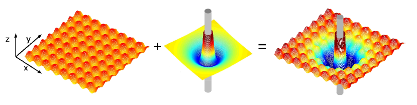
Figure 1: (Color online) Schematic showing a typical optical potential geometry resulting from the combination of an optical lattice potential and a trapping potential around an optical nano-fibre.

Optical Lattices typically have lattice constants in the range of $400$ nm to $650$ nm and we will consider a lattice with a trapping wavelength $\lambda/2=527$ nm. We choose the lattice to be loaded with ¹³³Cs atoms, which localize in the high field regions.

II.2 Sub-wavelength diameter optical fibres

Recent developments in tapered, dielectric fibre technology have made it possible to produce fibres with radii, $a$, as low as a few hundred nanometres Tong:03 . In such fibres the core has vanished and they can be described by one large refractive index step between the remaining cladding, $n_{1}(\omega)$, and the outside vacuum, $n_{2}$. An interesting consequence of the subwavelength nature of the diameter is that the majority of the field will be guided in the evanescent field on the fibre’s surface. It therefore becomes accessible to atoms in the fibre’s vicinity and light blue-detuned with respect to the atoms transition frequency will create a repulsive force preventing the atoms from coming too close to the fibre which is at room-temperature. At the same time red-detuned light will result in an attractive force and a combination of both fields was suggested by Le Kien et al. LeKien:04 as a way of creating a trapping potential around the fibre. This was experimentally observed in Vetsch:09 .

Let us briefly review the description of such a potential, following closely LeKien:04 . We consider two frequencies, $\omega_{r}$ and $\omega_{b}$, where the indices correspond to the red- and blue-detuned fields, respectively. They are chosen such that the single mode condition

$$V_{i}\equiv k_{i}a\sqrt{n_{1}^{2}(\omega)-n_{2}^{2}}<2.405\;,$$ (5)

is fulfilled Sellmeier and both light fields are in the fundamental mode HE₁₁. The intensity distribution of the evanescent fields depends on the polarization of the input fields and here we choose circular polarization for both beams to achieve angular symmetry Yariv:85 ; LeKien:04:2 . In cylindrical co-ordinates $\{r,\phi,\theta\}$, the time-averaged intensity outside the fibre is then given by

$$|E_{i}|^{2}=\epsilon_{i}^{2}\left[K_{0}^{2}(q_{i}r)+w_{i}K_{1}^{2}(q_{i}r)+f_{i}K_{2}^{2}(q_{i}r)\right].$$ (6)

Here the $K_{n}$ are the modified Bessel functions of the second kind and $\epsilon_{i}$ is the strength of the electric field. The decay of the fields from the surface of the fibre is characterized by $q_{i}$, which is the reciprocal of the decay length $\Lambda_{i}$ and given by

$$q_{i}=\sqrt{\beta_{i}^{2}-{n_{2}}^{2}{k_{i}}^{2}},$$ (7)

where $\beta$ is the longitudinal propagation constant of the mode Yariv:85 . Finally, the pre-factors are given by LeKien:04:2

$$w_{i} =\frac{2{q_{i}}^{2}}{\beta^{2}_{i}(1-s_{i})^{2}}\;,$$ (8)

$$f_{i} =\frac{(1+s_{i})^{2}}{(1-s_{i})^{2}}\;,$$ (9)

with $s$ defined as

$$s_{i}=\frac{\left(\frac{1}{q_{i}^{2}a^{2}}+\frac{1}{h_{i}^{2}a^{2}}\right)}{\left[\frac{J_{1}^{\prime}(h_{i}a)}{h_{i}aJ_{1}(h_{i}a)}+\frac{K_{1}^{\prime}(q_{i}a)}{q_{i}aK_{1}(q_{i}a)}\right]}\;,$$ (10)

and $h_{i}=(n_{1}^{2}k_{i}^{2}-\beta_{i}^{2})^{\frac{1}{2}}$. The combined optical potential around the fibre for a blue- and a red-detuned field is therefore given by (see Fig. 1)

$$U(r)= \frac{|\alpha_{b}|\varepsilon_{b}^{2}}{4}|\left[K_{0}^{2}(q_{b}r)+w_{b}K_{1}^{2}(q_{b}r)+f_{b}K_{2}^{2}(q_{b}r)\right]$$

$$-\frac{|\alpha_{r}|\varepsilon_{r}^{2}}{4}|\left[K_{0}^{2}(q_{r}r)+w_{r}K_{1}^{2}(q_{r}r)+f_{r}K_{2}^{2}(q_{r}r)\right]\;,$$ (11)

where the factors in front of the mode-structure terms are directly proportional to the powers of the individual light fields, $P_{r}$ and $P_{b}$.

II.3 Van der Waals interaction

Finally we need to take into account the van der Waals attraction between the atoms and the fibre. The classical van der Waals potential felt by an atom near the surface of a dielectric fibre of infinite length is given by Boustimi:02

$$V(r)=\frac{\hbar}{4\pi^{3}\epsilon_{0}}\sum_{n=-\infty}^{\infty} \int_{0}^{\infty}dk[k^{2}K_{n}^{{}^{\prime}}(kr)+(k^{2}+\frac{n^{2}}{r^{2}})K_{n}^{2}(kr)]$$

$$\times\int_{0}^{\infty}\!d\xi\;\alpha(i\xi)G_{n}(i\xi)\;,$$ (12)

where

$$G_{n}(\omega)=\frac{[\epsilon(\omega)-\epsilon_{0}]I_{n}(ka)I_{n}^{\prime}(ka)}{\epsilon_{0}I_{n}(ka)K_{n}^{\prime}(ka)-\epsilon(\omega)I_{n}^{\prime}(ka)K_{n}(ka)}\;.$$ (13)

Here the $I_{n}(x)$ and $K_{n}(x)$ are the modified Bessel function of the first and second kind, respectively. It should be noted that this approximation neglects the resonant frequencies of silica. However, as these are substantially different and weaker than those of Cs atoms, this is justified LeKien:04 .

A detailed analysis of expression (12) was carried out by Le Kien et al. LeKien:04 , who found that for atoms close to the surface the van der Waals potential tends to the same values as that for a flat surface. The latter has the simple and well known form

$$V_{\text{flat}}= -\frac{C_{3}}{(r-a)^{3}}\;,$$ (14)

$$C_{3}= \frac{\hbar}{16\pi^{2}\epsilon_{0}}\int_{0}^{\infty}\!d\xi\;\alpha(i\xi)[\frac{\epsilon(i\xi)-\epsilon_{0}}{\epsilon(i\xi)+\epsilon_{0}}]\;.$$ (15)

The ground state Caesium atom has its dominant ($D_{2}$) line at 852 nm, which gives a van der Waals constant of $C_{3}=2\pi\cdot 1.56$kHz $\mu$m³ Lauraspaper and this value will be used throughout this paper. In the following we will also use the simplified expression (14) whenever justified while making sure the full expression gives identical results.

III Scattering at the fibre

When a fibre is introduced in a position perpendicular to the transverse plane of a two-dimensional optical lattice, the four incident beams will be scattered from the cylindrical surface and distort the regularity of the lattice. To describe this we approximate the fibre by an infinite cylinder of radius $a=150$ nm oriented orthogonally to the lattice vectors and assume that the waves undergo a linear scattering process Kerker:69 . In cylindrical co-ordinates the four incident waves of the conventional lattice have the form of plane waves

$$\textbf{E}_{I}(\theta_{j})=\textbf{E}_{0}\exp\left[ikr\cos(\theta-\theta_{j})\right],$$ (16)

coming from the angles $\theta_{j}=0,\pi/2,\pi,3\pi/2$ and the total lattice field is that given by

$$E_{I}=\sqrt{\left(\textbf{E}_{I}(0)+\textbf{E}_{I}(\pi)\right)^{2}+\left(\textbf{E}_{I}\left(\frac{\pi}{2}\right)+\textbf{E}_{I}\left(\frac{3\pi}{2}\right)\right)^{2}}.$$ (17)

Assuming that the beams along the $\pi/2$-direction are polarized parallel to the cylinder axis and the ones along the $\pi$-direction orthogonal, the scattered field can be written as in Jones:73 , where the respective polarizations are contained in $E_{0}$.

$$E^{\parallel}_{S}=E_{0}\sum_{n=0}^{\infty}\Bigg{[} i^{n}a_{n}H_{n}^{(1)}(kr)\cos\left(n\left(\theta+\frac{\pi}{2}\right)\right)$$

$$+i^{n}a_{n}H_{n}^{(1)}(kr)\cos\left(n\left(\theta+\frac{3\pi}{2}\right)\right)\Bigg{]}$$ (18)

$$E^{\perp}_{S}=\frac{E_{0}}{kr}\sum_{n=0}^{\infty}\Bigg{[} i^{n}b_{n}H_{n}^{(1)}(kr)\cos(n\theta)$$

$$+i^{n}b_{n}H_{n}^{(1)}(kr)\cos(n(\theta+\pi))\Bigg{]}$$ (19)

where the $H_{n}^{(1)}$ are Hankel functions of the first kind and the scattering coefficients are given by

$$a_{n} =\frac{J_{n}(\alpha)J^{\prime}_{n}(m\alpha)-mJ_{n}(m\alpha)J^{\prime}_{n}(\alpha)}{H_{n}^{(2)}(\alpha)J^{\prime}_{n}(m\alpha)-mJ_{n}(m\alpha)H_{n}^{(2)^{\prime}}(\alpha)}\;,$$ (20)

$$b_{n} =\frac{mJ_{n}(\alpha)J^{\prime}_{n}(m\alpha)-J_{n}(m\alpha)J^{\prime}_{n}(\alpha)}{mH_{n}^{(2)}(\alpha)J^{\prime}_{n}(m\alpha)-J_{n}(m\alpha)H_{n}^{(2)^{\prime}}(\alpha)}\;.$$ (21)

From this the complete field follows as

$$E_{\text{tot}}=\sqrt{\left(E^{\parallel}_{I}+E^{\parallel}_{S}\right)^{2}+\left(E^{\perp}_{I}+E^{\perp}_{S}\right)^{2}}\;.$$ (22)

Here we note that all of the square plots in this paper span an area of 4.2 $\mu$m $\times$ 4.2 $\mu$m. This 4.2 $\mu$m corresponds to approximately four optical lattice wavelengths and thus an eight by eight grid of traps. The optical intensity in the vicinity of a fibre of radius $a=150$ nm for a lattice constant of $\lambda/2=527$ nm is shown in Figs. 2 (a) and (c). One can see that if the fibre is located at a minimum of the optical intensity (Fig. 2(a)), the lattice structure is almost unaffected. Positioning the fibre at an optical intensity maximum on the other hand (Fig. 2(c)) leads to noticeable disturbances, which, nevertheless, leave the basic lattice structure intact. Clearly larger fibres will lead to more scattering, however the numbers chosen here are well in reach of experimental possibilities.

In general the scattered radiation propagates as a cylindrical wave and its intensity falls off as the inverse power of the radial distance. Since the energy flow is only in the planes of constant $z$, the scattered radiation corresponding to a particular incident ray will be observed only in that plane which contains the incident ray and no scattering into other layers of a three-dimensional lattice occurs.

The overall potential seen by the atoms must include the van der Waals potential and Figs. 2(b) and (d) show that the lattice sites most affected by the scattering are also strongly affected by the van der Waals potential (Note that the Cs atoms we are considering here are high field seekers). It is clear that in a shallower lattice the effect of the van der Waals attraction will be more severe on a larger range and we will show in the next section that the introduction of a repulsive blue field can be a useful tool for counteracting this effect.

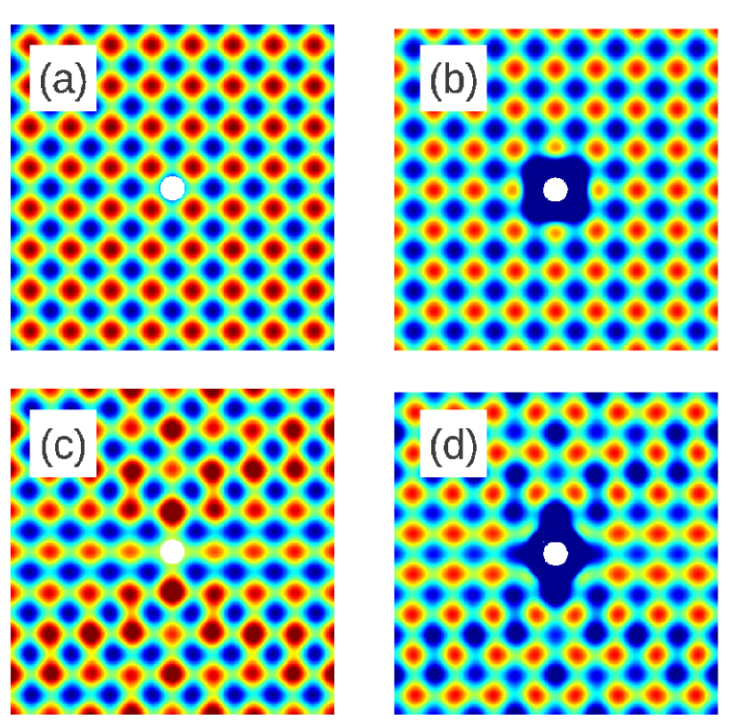
Figure 2: (Color online)(a) Lattice intensity including the scattering of the light on the fibre when the fibre is placed at an intensity minimum of the lattice. (b) van der Waals potential and optical lattice potential which includes the scattered lattice field. (c) and (d) show the same for a fibre placed at a lattice intensity maximum. Each plot spans an area of 4.2 $\mu$m $\times$ 4.2 $\mu$m and the lattice depth is 60 E_R. A colour scale has been used which varies from blue to red where the blue areas correspond to minima and red areas to maxima.

IV Adding fibre potentials

IV.1 Compensating the van der Waals potential

In order to minimize the disturbance of the lattice due to the van der Waals potential, we will study the possibility of compensating the attractive potential with a repulsive one from a blue-detuned optical field. The joint potential is simply given by adding the blue part of eq. (11) to the van der Waals expression of eq. (14)

$$U_{c}(r)= \frac{|\alpha_{b}|\varepsilon_{b}^{2}}{4}\left[K_{0}^{2}(q_{b}r)+w_{b}K_{1}^{2}(q_{b}r)+f_{b}K_{2}^{2}(q_{b}r)\right]$$

$$-\frac{C_{3}}{(r-a)^{3}}.$$ (23)

Since the modified Bessel functions have an exponentially decaying form it is not possible to perfectly compensate the van der Waals potential at all distances from the fibre. However, the discrepancy is weaker at larger distances, which allows the reduction of the radius in which the attractive potential is significant. In Figs. 3 and 4 we show the potential for the two different positions of the fibre for different intensities of the blue beam. One can clearly see that in both cases it is possible to achieve a situation in which almost all lattice sites close to the fibre are still intact (central panel). This is important for the construction of a well-defined Mott insulator state around the fibre, which is a prerequisite to loading the fibre potential with a well-defined particle number. While the exact number of restored lattice sites also depends on the lattice depth, the graphs show typical achievable experimental values. For very small distances from the fibre surface, the attractive van der Waals potential will always be stronger than the compensating optical field and tunnelling will become an important loss factor at longer times.

Let us also remark that with such a localized potential it is possible to remove atoms from specific lattice sites by using the fibre as a dark absorber Morrissey:09 . Used in conjunction with existing ideas involving optical conveyor belts Schrader:01 this simple setup could be an effective method of removing entire rows or patterns of atoms.

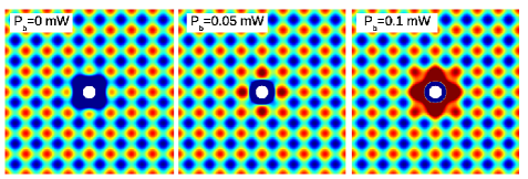
Figure 3: (Color online) Combined potentials (van der Waals, blue-detuned evanescent field and optical lattice) for a fibre placed at a minimum of the lattice intensity. The wavelength of the evanescent field is $\lambda_{b}=700$ nm and its power is increased through $P_{b}=$0, 0.05 and 0.10 mW from left to right. The lattice depth is chosen to be $=60E_{\text{rec}}$.

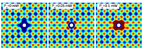
Figure 4: (Color online) Same as Fig. 3 with the fibre placed at a maximum of intensity of the lattice. Each plot spans an area of 4.2 $\mu$m $\times$ 4.2 $\mu$m.

IV.2 Loading the fibre potential

In the following we will consider the situation where an attractive, red-detuned field is added to the fibre as well. This will allow for the creation of a circular potential minimum around the fibre, deep enough to trap ultracold atoms. Recent experiments have demonstrated this by stochastically trapping atoms from a surrounding thermal or condensed cloud Vetsch:09 . Since in our situation the environment around the fibre is given by the well ordered optical lattice, a controlled melting of the lattice by the evanescent field will transfer a controllable number of atoms from the individual lattice sites into the fibre potential. The resulting state is therefore highly number squeezed and can be used in applications in quantum information or metrology Esteve:08 ; delcampo .

We study this process by assuming a realistic experimental situation of a Mott insulator made from Cs atoms with a resonant transition at $\lambda_{0}=852$ nm CesiumMott . For the two light fields in the fibre we consider a blue-detuned field at a wavelength of $\lambda_{b}=700$ nm and the red-detuned at $\lambda_{r}=980$ nm. The detunings of the fibre fields from the dominant line of the atom are then given by $\frac{\Delta_{b}}{2\pi}=-46$ THz and $\frac{\Delta_{r}}{2\pi}=76$ THz and with a fibre radius of $150$ nm, the evanescent decay lengths corresponding to the blue and red fields are $\Lambda_{b}=0.36~{}\mu$m and $\Lambda_{r}=1.83~{}\mu$m. The two-dimensional optical lattice we consider has a depth 60$E_{R}$.

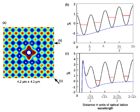
Figure 5: (Color online) (a) The black solid line represents the resulting two-dimensional potential geometry if the red and blue detuned beams in the fibre are switched on for $P_{b}=0.12$ mW and $P_{r}=0.036$ mW. The lattice sites for which the energy is lowered such that the residing atoms will be trapped in the fibre potential after the optical lattice is switched off are marked with a cross. (b) and (c) cut through the potential at the lines indicated in (a). The relevant on-site energies are indicated as well and the dotted blue line indicates the potential after the optical lattice is switched off. The fact that the fibre potential does not always meet exactly the zero points of the overall potential before switch-off is due to phase shifting of the optical lattice after scattering on the fibre.

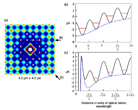
Figure 6: (Color online) Same as Fig. 5, but for higher powers of the evanescent fields, $P_{b}=0.17$ mW and $P_{r}=0.082$ mW. A larger number of atoms will be trapped after the optical lattice is switched off.

Two typical examples of resulting trapping geometries, when all potentials are taken into account, are shown in Figs. 5 and 6 for a fibre located at an intensity minimum. Since we assume the fibre to be initially dark, the lattice sites which are visible closest to the fibre in Figs. 5(c) and 6(c) are actually empty due to being within the radius of the surface’s van der Waals potential. For all other sites in the vicinity of the fibre one can clearly see that the addition of the red and blue fields allows for the lowering of the on-site energies. Therefore, as the asymptotic potential of the evanescent field goes to zero and since there is no local maximum in the fibre potential, a sudden switch off of the optical lattice will leave all atoms with centre-of-mass energies $<0$ trapped in the fibre potential alone. In the example shown in Fig. 5, where $P_{b}=0.12$ mW and $P_{r}=0.036$ mW, one finds that this condition is fulfilled for 8 lattice sites. Increasing the evanescent fields to $P_{b}=0.17$ mW and $P_{r}=0.082$ mW (see Fig. 6) the radius of the evanescent field increases and careful examination shows that 20 sites are reached. Note that, due to the rectangular geometry of the considered lattice, only certain atom numbers can be achieved and realistic parameters limit this technique to samples of only a few tens. If the switch-off process of the optical lattice is done on a time-scale shorter than the typical atom tunnelling time in an optical lattice (which is of the order of several milliseconds Greiner:02 ), no other atoms will have been able to join the well-defined sample.

The state created in this sudden-switch off procedure is a highly excited, out-of-equilibrium state in the final potential and subsequent cooling is necessary to prevent further atom loss due to scattering and thermalisation. While a detailed calculation of these effects go beyond the scope of this work, loss through re-thermalisation can be minimised by applying a Feshbach resonance while carrying out this process and subsequently adiabatically lowering the fibre potential while switching the interaction back on Alt:03 .

It is also worth pointing out that in both examples above the presence of the repulsive blue field ensures the existence of a repulsive wall between the fibre and the atoms, thereby preventing direct atom loss through the room temperature object. However, the power in the blue detuned field does not correspond to the same field strength that optimally cancels the effects of the van der Waals potential, as discussed in the previous chapter. It is rather necessary to over-compensate the van der Waals potential and recreate the trapping minimum using the red-detuned field. In the next section we will discuss the nature of the atomic state created in the fibre potential.

V Atomic State

Let us finally briefly characterise the atomic many-body state that can be created by the procedure above and focus in particular on the nature of the correlations in the sample. For this we first consider the effective dimensionality of the ground state of the potential around the fibre after the optical lattice is switched off. Since the size of the radial ground state of the potential will be much smaller than the curved, azimuthal one, we can assume an approximate separation of the wavefunction in the two directions. This allows us to describe the spectrum in the azimuthal direction by a free-space periodic potential with the well known spectrum $E_{n}^{a}=(n^{2}\hbar^{2}\pi^{2})/(2mL^{2})$, where $L=2\pi r_{m}$ is the circumference of the potential at the position of its radial minimum, $r_{m}$. Since no analytical expression for the position of this minimum is known, we find it numerically and estimate the energy difference between the ground and the first excited state in the azimuthal direction to be of the order of $\Delta E_{10}^{a}=E_{1}^{a}-E_{0}^{a}\sim 10^{-33}$ J, for both situations shown in Fig. 5

To find the spectrum in the radial direction, we numerically diagonalize the radial part of the potential for a wide range of parameters and find typical values for the separation of the ground and first excited state to be of the order of $\Delta E_{10}^{r}\sim 10^{-30}$ J. This significant difference in the stiffness of the spectra in the two different directions (the $z$-direction can be adjusted separately to be stiff) translates into an approximate one-dimensional situation with an aspect ratio of $\sim 10^{3}$.

Having established the effective dimensionality of the potential, the many body state of a one-dimensional Bose gas can now be characterized using the Lieb-Liniger parameter $\gamma=mg_{1D}/\hbar^{2}n_{1D}$ Lieb:63 . Here $g_{1D}$ is the one-dimensional coupling constant given by $g_{1D}=\frac{4\hbar^{2}a_{3D}}{ma_{\perp}}(a_{\perp}-Ca_{3D})^{-1}$ with $C\approx 1.4603$ and $n_{1D}$ is the linear density of the atoms Olshanii:98 . For values of $\gamma\gg 1$ the atomic many body state would be in the strongly correlated Tonks-Girardeau regime, whereas for $\gamma<1$ the gas can be treated as weakly correlated. For both cases shown in Fig. 5 the radial ground state size is of the order of $a_{\perp}\sim 0.2\;\mu$m (we assume the same is achieved in the z-direction) and the position of the radial minimum is at $r_{m}\sim 6.6\;\mu$m. This leads to values of $\gamma=0.560$ for the 8 atom case and $\gamma=0.346$ for the 20 atom case, putting both states firmly in the weakly correlated regime.

VI Conclusion

In this work we have suggested that the combination of optical lattices and tapered optical nano-fibres can be used to create small atomic samples which allow control over the final atom number. While introducing the fibre into the optical lattice inevitably leads to a disturbance of the lattice in the vicinity of the fibre due to scattering of the lattice beams, we have shown that this can be minimized and, due to the small fibre diameter, usually leaves the overall lattice structure intact. The attractive van der Waals potential close to the surface of the fibre can be compensated by using a blue-detuned evanescent field around the fibre, which allows a reduction of the range of the fibre’s influence to the size of a single lattice site for typical experimental parameters. Adding a second, red-detuned light field to the fibre then allows local melting of the optical lattice and can be used to create a small sample with a well-defined atom number. Finally, we have shown that these samples are in the superfluid regime and therefore good candidates for investigating the physics of persistent currents, or, using more varied optical potentials around the fibre, the physics of superfluid squids.