An M-estimator for tail dependence in arbitrary dimensions

Abstract

Consider a random sample in the max-domain of attraction of a multivariate extreme value distribution such that the dependence structure of the attractor belongs to a parametric model. A new estimator for the unknown parameter is defined as the value that minimizes the distance between a vector of weighted integrals of the tail dependence function and their empirical counterparts. The minimization problem has, with probability tending to one, a unique, global solution. The estimator is consistent and asymptotically normal. The spectral measures of the tail dependence models to which the method applies can be discrete or continuous. Examples demonstrate the applicability and the performance of the method.

, and

t1Supported by the Open Competition grant from the Netherlands Organisation for Scientific Research (NWO) and from the Deutsches Forschungsgemeinschaft (DFG) Grant SNF FOR 916. Research was mainly performed at Tilburg University and Eurandom (Eindhoven).

t2Supported by IAP research network Grant P6/03 of the Belgian government (Belgian Science Policy) and from the contract “Projet d’Actions de Recherche Concertées” no. 07/12/002 of the Communauté française de Belgique, granted by the Académie universitaire Louvain.

1 Introduction

Statistics of multivariate extremes finds important applications in fields like finance, insurance, environmental sciences, aviation safety, hydrology and meteorology. When considering multivariate extreme events, the estimation of the tail dependence structure is the key part of the statistical inference. This tail dependence structure, represented by the stable tail dependence function $l$, becomes rather complex if the dimension increases. Therefore, it is customary to model this multivariate function $l$ parametrically, which leads to a semiparametric model. The interest in parametric tail dependence models has existed since the early sixties of the 20th century [Gumbel (1960)], but new models are still being proposed [Boldi and Davison (2007), Cooley, Davis and Naveau (2010), Ballani and Schlather (2011)]. Most of the existing estimators of the parameter, $\theta$, are likelihood-based and their asymptotic behavior is only known in dimension two [Coles and Tawn (1991), Joe, Smith and Weissman (1992), Smith (1994), Ledford and Tawn (1996), de Haan, Neves and Peng (2008), Guillotte, Perron and Segers (2011)]. For many applications, the bivariate setup is too restrictive. Also, the likelihood-based estimation methods exclude models that entail a nondifferentiable function $l$, like the widely used factor models; see (1) below.

It is the goal of this paper to present and provide a comprehensive treatment of novel M-estimators of $\theta$. The estimators can be used in arbitrary dimension $d$. Moreover, not relying on the differentiability of $l$, the estimators are broadly applicable. We establish, again for arbitrary dimension $d$, the asymptotic normality of our estimators, which yields asymptotic confidence regions and tests for the parameter $\theta$. The results in this paper make statistical inference possible for many multivariate extreme value models that either cannot be handled at all by currently available methods or for which statistical theory has only been provided for the bivariate case. Monte Carlo simulation studies confirm that our estimators perform well in practice; see Sections 5 and 6.

The present estimators are a major extension of the method of moments estimators for dimension two [Einmahl, Krajina and Segers (2008)]. For applications, the crucial difference is that it is now possible to handle truly multivariate data. Also, theoretically, extreme value analysis in dimensions larger than two is quite challenging, which explains why in many papers attention is restricted to the bivariate case. In particular, we establish the asymptotic behavior of the nonparametric estimator of $l$ in arbitrary dimensions and under nonrestrictive smoothness conditions; compare, for instance, with Drees and Huang (1998) in the bivariate case. Another novel aspect is that the method of moments technique is replaced by general M-estimation, that is, allowing for more estimating equations than the dimension of the parameter space. This more flexible procedure may serve to increase the efficiency of the estimator.

The absence of smoothness assumptions on $l$ makes it possible to estimate the tail dependence structure of factor models like $X=(X_{1},\ldots,X_{d})$, with

$$X_{j}=\sum_{i=1}^{r}a_{ij}Z_{i}+\varepsilon_{j},\qquad j=1,\ldots,d,$$ (1)

consisting of the following ingredients: nonnegative factor loadings $a_{ij}$ and independent, heavy-tailed random variables $Z_{i}$ called factors; independent random variables $\varepsilon_{j}$ whose tails are lighter than the ones of the factors and which are independent of them. This kind of factor model is often used in finance, for example, in modeling market or credit risk [Fama and French (1993), Malevergne and Sornette (2004), Geluk, de Haan and de Vries (2007)]. From equation (28) below, we see that the stable tail dependence function $l$ of such a factor model is not everywhere differentiable, causing likelihood-based methods to break down.

The organization of the paper is as follows. The basics of the tail dependence structures in multivariate models are presented in Section 2. The M-estimator is defined in Section 3. Section 4 contains the main theoretical results: consistency and asymptotic normality of the M-estimator, and some consequences of the asymptotic normality result that can be used for construction of confidence regions and for testing. This section also contains the asymptotic normality result for $\hat{l}_{n}$. In Section 5 we apply the M-estimator to the well-known logistic stable tail dependence function (23). The tail dependence structure of factor models is studied in Section 6. Both models are illustrated with simulated and real data. The proofs are deferred to Section 7.

2 Tail dependence

We will write points in ${\mathbb{R}}^{d}$ as $x=(x_{1},\ldots,x_{d})$ and random vectors as $X_{i}=(X_{i1},\ldots,X_{id})$, for $i=1,\ldots,n$. Let $X_{1},\ldots,X_{n}$ be independent random vectors in ${\mathbb{R}}^{d}$ with common continuous distribution function $F$ and marginal distribution functions $F_{1},\ldots,F_{d}$. For $j=1,\ldots,d$, write $M_{n}^{(j)}:=\max_{i=1,\ldots,n}X_{ij}$. We say that $F$ is in the max-domain of attraction of an extreme value distribution $G$ if there exist sequences $a_{n}^{(j)}>0$, $b_{n}^{(j)}\in{\mathbb{R}}$, $j=1,\ldots,d$, such that

$$\lim_{n\to\infty}{\mathbb{P}}\biggl{(}\frac{M_{n}^{(1)}-b_{n}^{(1)}}{a_{n}^{(1)}}\leq x_{1},\ldots,\frac{M_{n}^{(d)}-b_{n}^{(d)}}{a_{n}^{(d)}}\leq x_{d}\biggr{)}=G(x)$$ (2)

for all continuity points $x\in{\mathbb{R}}^{d}$ of $G$. The margins $G_{1},\ldots,G_{d}$ of $G$ must be univariate extreme value distributions and the dependence structure of $G$ is determined by the relation

$$-\log G(x)=l\bigl{(}-\log G_{1}(x_{1}),\ldots,-\log G_{d}(x_{d})\bigr{)}$$

for all points $x$ such that $G_{j}(x_{j})>0$ for all $j=1,\ldots,d$. The stable tail dependence function $l\dvtx[0,\infty)^{d}\to[0,\infty)$ can be retrieved from $F$ via

$$\qquad l(x)=\lim_{t\downarrow 0}t^{-1}{\mathbb{P}}\bigl{\{}1-F_{1}(X_{11})\leq tx_{1}\mbox{ or }\ldots\mbox{ or }1-F_{d}(X_{1d})\leq tx_{d}\bigr{\}}.$$ (3)

In fact, the joint convergence in (2) is equivalent to convergence of the $d$ marginal distributions together with (3).

In this paper we will only assume the weaker relation (3). By itself, (3) holds if and only if the random vector $(1/\{1-F_{1}(X_{1j})\})_{j=1}^{d}$ belongs to the max-domain of attraction of the extreme value distribution $G_{0}(x)=\exp\{-l(1/x_{1},\ldots,1/x_{d})\}$ for $x\in(0,\infty)^{d}$. Alternatively, the existence of the limit in (3) is equivalent to multivariate regular variation of the random vector $(1/\{1-F_{1}(X_{1j})\})_{j=1}^{d}$ on the cone $[0,\infty]^{d}\setminus\{(0,\ldots,0)\}$ with limit measure or exponent measure $\mu$ given by

$$\mu\bigl{(}\bigl{\{}z\in[0,\infty]^{d}\dvtx z_{1}\geq x_{1}\mbox{ or }\ldots\mbox{ or }z_{d}\geq x_{d}\bigr{\}}\bigr{)}=l(1/x_{1},\ldots,1/x_{d})$$

[Resnick (1987), Beirlant et al. (2004), de Haan and Ferreira (2006)]. The measure $\mu$ is homogeneous, that is, $\mu(tA)=t^{-1}\mu(A)$, for any $t>0$ and any relatively compact Borel set $A\subset[0,\infty]^{d}\setminus\{(0,\ldots,0)\}$, where $tA:=\{tz\dvtx z\in A\}$. This homogeneity property yields a decomposition of $\mu$ into a radial and an angular part [de Haan and Resnick (1977), Resnick (1987)]. Let $\Delta_{d-1}:=\{w\in[0,1]^{d}\dvtx w_{1}+\cdots+w_{d}=1\}$ be the unit simplex in ${\mathbb{R}}^{d}$. Associated to $B\subset\Delta_{d-1}$ and $t>0$ is the set

$$B_{t}=\Biggl{\{}x\in[0,\infty)^{d}\setminus\bigl{\{}(0,\ldots,0)\bigr{\}}\dvtx{\sum_{j=1}^{d}}x_{j}\geq t,x\Big{/}{\sum_{j=1}^{d}}x_{j}\in B\Biggr{\}}.$$

By the homogeneity property of the exponent measure, it holds that $\mu(B_{t})=t^{-1}\mu(B_{1})$. Writing $H(B)=\mu(B_{1})$ defines a finite measure $H$ on $\Delta_{d-1}$, called the spectral or angular measure. Any finite measure satisfying the moment conditions

$$\int_{\Delta_{d-1}}w_{j}H(\mathrm{d}w)=1,\qquad j=1,\ldots,d,$$ (4)

is a spectral measure. Adding up the $d$ constraints in (4) shows that $H/d$ is a probability measure.

Sometimes it is more convenient to work with the measure $\Lambda$ obtained from $\mu$ after the transformation $(x_{1},\ldots,x_{d})\mapsto(1/x_{1},\ldots,1/x_{d})$. The measure $\Lambda$ is also called the exponent measure and it satisfies the homogeneity property $\Lambda(tA)=t\Lambda(A)$, for any $t>0$ and Borel set $A\subset[0,\infty]^{d}\setminus\{(\infty,\ldots,\infty)\}$.

There is a one-to-one correspondence between the stable tail dependence function $l$, the exponent measures $\mu$ and $\Lambda$, and the spectral measure $H$. In particular, we have

$$\qquad l(x) = \mu\bigl{(}\bigl{\{}(z_{1},\ldots,z_{d})\in[0,\infty]^{d}\dvtx z_{1}\geq 1/x_{1}\mbox{ or }\ldots\mbox{ or }z_{d}\geq 1/x_{d}\bigr{\}}\bigr{)}$$ (5)

$$= \Lambda\bigl{(}\bigl{\{}(u_{1},\ldots,u_{d})\in[0,\infty]^{d}\dvtx u_{1}\leq x_{1}\mbox{ or }\ldots\mbox{ or }u_{d}\leq x_{d}\bigr{\}}\bigr{)}$$ (6)

$$= \int_{\Delta_{d-1}}\max_{j=1,\ldots,d}\{w_{j}x_{j}\}H(\mathrm{d}w).$$ (7)

From the above representations and the moment constraints (4), it follows that the function $l$ has the following properties:

• $\max\{x_{1},\ldots,x_{d}\}\leq l(x)\leq x_{1}+\cdots+x_{d}$ for all $x\in[0,\infty)^{d}$; in particular, $l(z,0,\ldots,0)=\cdots=l(0,\ldots,0,z)=z$ for all $z\geq 0$;

• $l$ is convex; and

• $l$ is homogeneous of order one: $l(tx_{1},\ldots,tx_{d})=tl(x_{1},\ldots,x_{d})$, for all $t>0$ and all $x\in[0,\infty)^{d}$.

The function $l$ is connected to the function $V$ in Coles and Tawn (1991) through $l(x)=V(1/x_{1},\ldots,1/x_{d})$ for $x\in(0,\infty)^{d}$.

The right-hand partial derivatives of $l$ always exist; indeed, by bounded convergence it follows that for $j=1,\ldots,d$, as $h\downarrow 0$,

$$\frac{1}{h}\bigl{(}l(x_{1},\ldots,x_{j-1},x_{j}+h,x_{j+1},\ldots,x_{d})-l(x_{1},\ldots,x_{j-1},x_{j},x_{j+1},\ldots,x_{d})\bigr{)}$$

$$\qquad=\int_{\Delta_{d-1}}\frac{1}{h}\Bigl{(}\max\Bigl{\{}w_{j}x_{j}+w_{j}h,\max_{s\neq j}\{w_{s}x_{s}\}\Bigr{\}}$$

(8)

$$\hskip 93.1pt{}-\max\Bigl{\{}w_{j}x_{j},\max_{s\neq j}\{w_{s}x_{s}\}\Bigr{\}}\Bigr{)}H(\mathrm{d}{w})$$

$$\qquad\to\int_{\Delta_{d-1}}w_{j}\mathbf{1}\Bigl{\{}w_{j}x_{j}\geq\max_{s\neq j}\{w_{s}x_{s}\}\Bigr{\}}H(\mathrm{d}{w}).$$

Similarly, the left-hand partial derivatives exist for all $x\in(0,\infty)^{d}$. By convexity, the function $l$ is almost everywhere continuously differentiable, with its gradient vector of (the right-hand) partial derivatives as in (2).

3 Estimation

Let $R_{i}^{j}$ denote the rank of $X_{ij}$ among $X_{1j},\ldots,X_{nj}$, $i=1,\ldots,n$, $j=1,\ldots,d$. For $k\in\{1,\ldots,n\}$, define a nonparametric estimator of $l$ by

$$\hat{l}_{n}(x) = \hat{l}_{k,n}(x)$$

$$:\! = \frac{1}{k}\sum_{i=1}^{n}\mathbf{1}\biggl{\{}R_{i}^{1}>n+\frac{1}{2}-kx_{1}\mbox{ or }\ldots\mbox{ or }R_{i}^{d}>n+\frac{1}{2}-kx_{d}\biggr{\}};$$

see Huang (1992) and Drees and Huang (1998) for the bivariate case. This definition follows from (3), with all the distribution functions replaced by their empirical counterparts, and with $t$ replaced by $k/n$. Here $k=k_{n}$ is such that $k\to\infty$ and $k/n\to 0$ as $n\to\infty$. The constant $1/2$ in the argument of the indicator function helps to improve the finite-sample properties of the estimator.

In the literature, the stable tail dependence function is often modeled parametrically. We impose that the stable tail dependence function $l$ belongs to some parametric family $\{l(\cdot;\theta)\dvtx\theta\in\Theta\}$, where $\Theta\subset{\mathbb{R}}^{p}$, $p\geq 1$. Note that this is still a large, flexible model since there is no restriction on the marginal distributions and the copula is constrained only through $l$; see (3).

We propose an M-estimator of $\theta$. Let $q\geq p$. Let $g\equiv(g_{1},\ldots,g_{q})^{T}\dvtx[0,1]^{d}\to{\mathbb{R}}^{q}$ be a column vector of integrable functions such that $\varphi\dvtx\Theta\to{\mathbb{R}}^{q}$ defined by

$$\varphi(\theta):=\int_{[0,1]^{d}}g(x)l(x;\theta)\,\mathrm{d}x$$ (10)

is a homeomorphism between $\Theta$ and its image $\varphi(\Theta)$. Let $\theta_{0}$ denote the true parameter value. The M-estimator $\hat{\theta}_{n}$ of $\theta_{0}$ is defined as a minimizer of the criterion function

$$\quad Q_{k,n}(\theta)=\biggl{\|}\varphi(\theta)-\int g\hat{l}_{n}\biggr{\|}^{2}=\sum_{m=1}^{q}\biggl{(}\int_{[0,1]^{d}}g_{m}(x)\bigl{(}\hat{l}_{n}(x)-l(x;\theta)\bigr{)}\,\mathrm{d}x\biggr{)}^{2},$$ (11)

where $\|\cdot\|$ is the Euclidean norm. In other words, if $\hat{Y}_{n}={\mathop{\arg\min}_{y\in\varphi(\Theta)}}\|y-\int g\hat{l}_{n}\|$, then $\hat{\theta}_{n}\in\varphi^{-1}(\hat{Y}_{n})$. Later we show that $\hat{\theta}_{n}$ is, with probability tending to one, unique.

The fact that our model assumption only concerns a limit relation in the tail shows up in the estimation procedure through the choice of $k$, which determines the effective sample size. When we study asymptotic properties of either $\hat{l}_{n}$ or $\hat{\theta}_{n}$, $k=k_{n}$ is an intermediate sequence, that is, $k\to\infty$ and $k/n\to 0$ as $n\to\infty$. In practice, the choice of optimal $k$ is a notorious problem, and here we address this issue in the usual way: we present the finite sample results over a wide range of $k$; see Sections 5 and 6.

Remark 3.1.

The estimator $\hat{\theta}_{n}$ depends on $g$. In line with the classical method of moments and for computational feasibility, we will choose $g$ to be a vector of low degree polynomials. In Sections 5 and 6 we will see that the obtained estimators have a good performance and a wide applicability. Finding an optimal $g$ is very difficult and statistically not very useful since such a $g$ depends on the true, unknown $\theta_{0}$. For example, when $p=q=1$, a function $g$ that minimizes the asymptotic variance is $(\partial/\partial\theta)l(x;\theta_{0})$. For two-dimensional and five-dimensional data, a sensitivity analysis on the choice of $g$ is performed in Section 5. Simple functions like $1$ or $x_{1}$ lead to estimators that perform approximately the same as the pseudo-estimator based on the optimal $g$. This supports our choices of $g$ and also suggests that the estimator is not so sensitive to the choice of $g$.

Remark 3.2.

Since $l$, part of the model, is parametrically specified, in principle, pseudo maximum likelihood estimation could be used. This method, however, does not apply to many interesting models where $l$ is not differentiable, like the factor model in (1). Moreover, no theory is known for dimensions higher than 2, unless the limit relation (3) is replaced by an equality for all sufficiently small $t$. In this paper, the emphasis is on higher dimensions and for a large part on the factor model. Therefore, the pseudo MLE is not an available competitor.

4 Asymptotic results

Let $\hat{\Theta}_{n}$ be the set of minimizers of $Q_{k,n}$ in (11), that is,

$$\hat{\Theta}_{n}:=\mathop{\arg\min}_{\theta\in\Theta}\biggl{\|}\varphi(\theta)-\int g\hat{l}_{n}\biggr{\|}^{2}.$$

Note that $\hat{\Theta}_{n}$ may be empty or may contain more than one element. We show that under suitable conditions, a minimizer exists, that it is unique with probability tending to one, and that it is a consistent and asymptotically normal estimator of $\theta_{0}$. In addition, we show that the nonparametric estimator $\hat{l}_{n}$ in (3) is asymptotically normal.

4.1 Notation

Recall the definition of the measure $\Lambda$ from Section 2. Let $W_{\Lambda}$ be a mean-zero Wiener process indexed by Borel sets of $[0,\infty]^{d}\setminus\{(\infty,\ldots,\infty)\}$ with “time” $\Lambda$: its covariance structure is given by

$$\mathbb{E}\bigl{[}W_{\Lambda}(A_{1})W_{\Lambda}(A_{2})\bigr{]}=\Lambda(A_{1}\cap A_{2})$$ (12)

for any two Borel sets $A_{1}$ and $A_{2}$ in $[0,\infty]^{d}\setminus\{(\infty,\ldots,\infty)\}$. Define

$$W_{l}(x):=W_{\Lambda}\bigl{(}\bigl{\{}u\in[0,\infty]^{d}\setminus\bigl{\{}(\infty,\ldots,\infty)\bigr{\}}\dvtx u_{1}\leq x_{1}\mbox{ or }\ldots\mbox{ or }u_{d}\leq x_{d}\bigr{\}}\bigr{)}.$$ (13)

Let $W_{l,j},j=1,\ldots,d$, be the marginal processes

$$W_{l,j}(x_{j}):=W_{l}(0,\ldots,0,x_{j},0,\ldots,0),\qquad x_{j}\geq 0.$$ (14)

Define $l_{j}$ to be the right-hand partial derivative of $l$ with respect to $x_{j}$, where $j=1,\ldots,d$ [see (2)]; if $l$ is differentiable, $l_{j}$ is equal to the corresponding partial derivative of $l$. Write

$$\qquad B(x):=W_{l}(x)-\sum_{j=1}^{d}l_{j}(x)W_{l,j}(x_{j}),\qquad\tilde{B}:=\int_{[0,1]^{d}}g(x)B(x)\,\mathrm{d}x.$$ (15)

The distribution of $\tilde{B}$ is zero-mean Gaussian with covariance matrix

$$\Sigma:=\int\!\!\int_{([0,1]^{d})^{2}}\mathbb{E}\bigl{[}B(x)B(y)\bigr{]}g(x)g(y)^{T}\,\mathrm{d}x\,\mathrm{d}y\in{\mathbb{R}}^{q\times q}.$$ (16)

Note that if $l$ is parametric, $\Sigma$ depends on the parameter, that is, $\Sigma=\Sigma(\theta)$.

Assuming $\theta$ is an interior point of $\Theta$ and $\varphi$ is differentiable in $\theta$, let $\dot{\varphi}(\theta)\in{\mathbb{R}}^{q\times p}$ be the total derivative of $\varphi$ at $\theta$, and, provided $\dot{\varphi}(\theta)$ is of full rank, put

$$M(\theta):=\bigl{(}\dot{\varphi}(\theta)^{T}\dot{\varphi}(\theta)\bigr{)}^{-1}\dot{\varphi}(\theta)^{T}\Sigma(\theta)\dot{\varphi}(\theta)\bigl{(}\dot{\varphi}(\theta)^{T}\dot{\varphi}(\theta)\bigr{)}^{-1}\in{\mathbb{R}}^{p\times p}.$$ (17)

4.2 Results

We state the asymptotic results for the M-estimator, $\hat{\theta}_{n}$, and the asymptotic normality of $\hat{l}_{n}$. The latter is a result of independent interest, and requires continuous partial derivatives of $l$, which is not an assumption for the asymptotic normality of the M-estimator. The proofs can be found in Section 7.

Theorem 4.1 ((Existence, uniqueness and consistency of $\hat{\theta}_{n}$))

Let $g\dvtx\break[0,1]^{d}\to{\mathbb{R}}^{q}$ be integrable. [(ii)]

If $\varphi$ is a homeomorphism from $\Theta$ to $\varphi(\Theta)$ and if there exists $\varepsilon_{0}>0$ such that the set $\{\theta\in\Theta\dvtx\|\theta-\theta_{0}\|\leq\varepsilon_{0}\}$ is closed, then for every $\varepsilon$ such that $\varepsilon_{0}\geq\varepsilon>0$, as $n\to\infty$,

$${\mathbb{P}}\bigl{(}\hat{\Theta}_{n}\neq\varnothing\mbox{ and }\hat{\Theta}_{n}\subset\bigl{\{}\theta\in\Theta\dvtx\|\theta-\theta_{0}\|\leq\varepsilon\bigr{\}}\bigr{)}\to 1.$$

If in addition to the assumptions of (i), $\theta_{0}$ is in the interior of the parameter space, $\varphi$ is twice continuously differentiable and $\dot{\varphi}(\theta_{0})$ is of full rank, then, with probability tending to one, $Q_{k,n}$ in (11) has a unique minimizer $\hat{\theta}_{n}$. Hence,

$$\hat{\theta}_{n}\stackrel{{\scriptstyle{\mathbb{P}}}}{{\to}}\theta_{0}\qquad\mbox{as }n\to\infty.$$

In part (i) of this theorem we assume that the set $\{\theta\in\Theta\dvtx\|\theta-\theta_{0}\|\leq\varepsilon\}$ is closed for some $\varepsilon>0$. This is a generalization of the usual assumption that $\Theta$ is open or closed, and includes a wider range of possible parameter spaces.

Theorem 4.2 ((Asymptotic normality of $\hat{\theta}_{n}$))

If in addition to the assumptions of Theorem 4.1(ii), the following two conditions hold: [(C2)]

$t^{-1}{\mathbb{P}}\{1-F_{1}(X_{11})\leq tx_{1}\mbox{ or }\ldots\mbox{ or }1-F_{d}(X_{1d})\leq tx_{d}\}-l(x)=O(t^{\alpha})$, uniformly in $x\in\Delta_{d-1}$ as $t\downarrow 0$, for some $\alpha>0$,

$k=o(n^{2\alpha/(1+2\alpha)})$, for the positive number $\alpha$ of (C1), and $k\to\infty$ as $n\to\infty$, then as $n\to\infty$, with $M$ as in (17),

$$\sqrt{k}(\hat{\theta}_{n}-\theta_{0})\stackrel{{\scriptstyle d}}{{\to}}N\bigl{(}0,M(\theta_{0})\bigr{)}.$$ (18)

The following consequence of Theorem 4.2 can be used for the construction of confidence regions. Recall from (7) that $H_{\theta}$ is the spectral measure corresponding to $l(\cdot;\theta)$. Let $\chi^{2}_{\nu}$ denote the $\chi^{2}$-distribution with $\nu$ degrees of freedom.

Corollary 4.3

If in addition to the conditions of Theorem 4.2, the map $\theta\mapsto H_{\theta}$ is weakly continuous at $\theta_{0}$ and if the matrix $M(\theta_{0})$ is nonsingular, then as $n\to\infty$,

$$k(\hat{\theta}_{n}-\theta_{0})^{T}M(\hat{\theta}_{n})^{-1}(\hat{\theta}_{n}-\theta_{0})\stackrel{{\scriptstyle d}}{{\to}}\chi^{2}_{p}.$$ (19)

Let $1\leq r<p$ and $\theta=(\theta_{1},\theta_{2})\in\Theta\subset{\mathbb{R}}^{p}$, where $\theta_{1}\in{\mathbb{R}}^{p-r}$, $\theta_{2}\in{\mathbb{R}}^{r}$. We want to test $\theta_{2}=\theta_{2}^{*}$ against $\theta_{2}\neq\theta_{2}^{*}$, where $\theta_{2}^{*}$ corresponds to a submodel. Denote $\hat{\theta}_{n}=(\hat{\theta}_{1n},\hat{\theta}_{2n})$, and let $M_{2}(\theta)$ be the $r\times r$ matrix corresponding to the lower right corner of $M$, as below:

$$M=\pmatrix{\cdots\hskip 2.0pt|\hskip 2.0pt\cdots\cr\hline\cr\cdots\hskip 2.0pt|\hskip 1.0ptM_{2}}\in{\mathbb{R}}^{p\times p}.$$ (20)

Corollary 4.4 ((Test))

If the assumptions of Corollary 4.3 are satisfied, and $\theta_{0}=(\theta_{1},\theta_{2}^{*})\in\Theta$ for some $\theta_{1}$, then as $n\to\infty$,

$$k\bigl{(}\hat{\theta}_{2n}-\theta_{2}^{*}\bigr{)}^{T}M_{2}\bigl{(}\hat{\theta}_{1n},\theta_{2}^{*}\bigr{)}^{-1}\bigl{(}\hat{\theta}_{2n}-\theta_{2}^{*}\bigr{)}\stackrel{{\scriptstyle d}}{{\to}}\chi_{r}^{2}.$$ (21)

The above result can be used for testing for a submodel. For example, we could test for the symmetric logistic model of (25) within the asymmetric logistic one; see Section 5.

Remark 4.5.

The matrices $M$ and $M_{2}$ are needed for the computation of the confidence regions and the test statistics. However, computing these matrices can be challenging. To compute $M$, we first need the $q\times p$ matrix $\dot{\varphi}(\theta)$, whose $(i,j)$th element is given by $\int g_{i}(x)(\partial/\partial\theta_{j})l(x;\theta)\,\mathrm{d}x$. The expression itself will depend on the model in use, but usually the (right-hand) partial derivatives of $l$ can be computed explicitly, whereas the integral is to be computed numerically in most cases. Second, we need to calculate the covariance of the process $\tilde{B}$. We see from (16) that the most difficult part will be the expression $\mathbb{E}[B(x)B(y)]$. It holds that

$$\mathbb{E}\bigl{[}B(x)B(y)\bigr{]} = \mathbb{E}\bigl{[}W_{l}(x)W_{l}(y)\bigr{]}-\sum_{j=1}^{d}l_{j}(y)\mathbb{E}\bigl{[}W_{l}(x)W_{l,j}(y_{j})\bigr{]}$$

$${}-\sum_{i=1}^{d}l_{i}(x)\mathbb{E}\bigl{[}W_{(l,i)}(x_{i})W_{l}(y)\bigr{]}$$

$${}+\sum_{i=1}^{d}\sum_{j=1}^{d}l_{i}(x)l_{j}(y)\mathbb{E}\bigl{[}W_{(l,i)}(x_{i})W_{l,j}(y_{j})\bigr{]}.$$

Using (12), (13), (14) and the relation between $\Lambda$ and $l$, we can express this in $l$ and its partial derivatives. Numerical integration is then performed to obtain $\Sigma$.

Finally, we show the asymptotic normality of $\hat{l}_{n}$. This result is of independent interest and can be found in the literature for $d=2$ only and under stronger smoothness conditions on $l$; see Huang (1992), Drees and Huang (1998) and de Haan and Ferreira (2006). Here, a large part of its proof is necessary for the proof of the asymptotic normality of $\hat{\theta}_{n}$, but we wish to emphasize that the asymptotic normality of $\hat{\theta}_{n}$ holds without any differentiability conditions on $l$. Note that under assumption (C3) below, the process $B$ in (15) is continuous, although $l_{j}$ may be discontinuous at points $x$ such that $x_{j}=0$.

The result is stated in an approximation setting, where $\hat{l}_{n}$ and $B$ are defined on the same probability space obtained by a Skorohod construction. The random quantities involved are only in distribution equal to the original ones, but for convenience this is not expressed in the notation.

Theorem 4.6 ((Asymptotic normality of $\hat{l}_{n}$ in arbitrary dimensions))

If in addition to the conditions (C1) and (C2) from Theorem 4.2, the following condition holds:

[(C3)]

for all $j=1,\ldots,d$, the first-order partial derivative of $l$ with respect to $x_{j}$ exists and is continuous on the set of points $x$ such that $x_{j}>0$, then for every $T>0$, as $n\to\infty$,

$$\sup_{x\in[0,T]^{d}}\bigl{|}\sqrt{k}\bigl{(}\hat{l}_{n}(x)-l(x)\bigr{)}-B(x)\bigr{|}\stackrel{{\scriptstyle{\mathbb{P}}}}{{\to}}0.$$ (22)

5 Example 1: Logistic model

The multivariate logistic distribution function with standard Fréchet margins is defined by

$$F(x_{1},\ldots,x_{d};\theta)=\exp\Biggl{\{}-\Biggl{(}{\sum_{j=1}^{d}}x_{j}^{-1/\theta}\Biggr{)}^{\theta}\Biggr{\}}$$

for $x_{1}>0,\ldots,x_{d}>0$ and $\theta\in[0,1]$, with the proper limit interpretation for $\theta=0$. The corresponding stable tail dependence function is given by

$$l(x_{1},\ldots,x_{d};\theta)=\bigl{(}x_{1}^{1/\theta}+\cdots+x_{d}^{1/\theta}\bigr{)}^{\theta}.$$ (23)

Introduced in Gumbel (1960), it is one of the oldest parametric models of tail dependence.

Sensitivity analysis

Here we observe how for the logistic model the M-estimator changes with different choices of $k$, and for different functions $g$. Within this model, $p=1$ and in the simple case of $p=q=1$, it is easy to see that the optimal choice for the function $g$ is $(\partial/\partial\theta)l(x;\theta_{0})$. Since it depends on the unknown true parameter, this is not a viable option for use in practice, but, as demonstrated below, some simple alternatives result in estimators with basically the same finite-sample behavior.

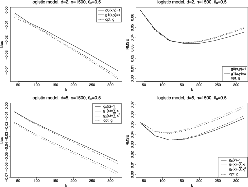
Figure 1: Logistic model: the M-estimator for different functions $g$ in dimension $d=2$ (top) and $d=5$ (bottom).

The following analysis is performed for the logistic model with $\theta_{0}=0.5$, in dimensions 2 and 5. For both settings, we look at 200 replications of samples of size $n=1500$, and take the threshold parameters $k\in\{40,80,\ldots,320\}$. In the bivariate case we compare $g_{0}(x_{1},x_{2})=1$, $g_{1}(x_{1},x_{2})=x_{1}$ and $g_{\mathrm{opt}}(x_{1},\break x_{2})=(\partial/\partial\theta)l(x_{1},x_{2};\theta_{0})$ as choices for $g$. In the five-dimensional case the functions $g_{0}$ and $g_{\mathrm{opt}}$ are defined analogously, and we compare them to two other functions, $g_{1}(x)=\sum_{j=1}^{5}x_{j}$ and $g_{2}(x)=\sum_{j=1}^{5}x_{j}^{2}$. We use the bias and the Root Mean Squared Error (RMSE) to assess the performance of the estimators. The results are presented in Figure 1 for dimensions $d=2$ (top) and $d=5$ (bottom). All of the above choices for $g$ result in similar finite-sample behavior of the estimator, but the simpler function $g$ leads to a somewhat better performance. The RMSEs for some of these $g$ are even lower than the one for $g_{\mathrm{opt}}$, since they yield a smaller bias.

Based on these findings, for the logistic model in dimensions $2$ and $5$, we advise the use of the simplest choice of $g$ given by $g_{0}(x)=1$, for all $x\geq 0$. The choice of $k$ is slightly more delicate, but it seems that for $n=1500$ in dimensions 2 and 5, the choices of $k=150$ and $k=100$, respectively, are reasonable.

Comparison with maximum likelihood based estimators

For $d=2$, we also compare the M-estimator with $g\equiv 1$ with the censored maximum likelihood method [see Ledford and Tawn (1996)] and with the maximum likelihood estimator introduced in de Haan, Neves and Peng (2008). The latter two we will call the censored MLE and the dHNP MLE, respectively. For 200 samples, we compute the censored MLE using the function fitbvgpd from the R package POT [see Ribatet (2011)]; the dHNP MLE is calculated as described in the original article. Since the thresholds used in these two methods differ, and since for a different choice of threshold we get a different estimator, the comparison is not straightforward. We consider the M-estimator and the dHNP MLE over the range of $k$ values as used above, and for the censored MLE we take the thresholds such that the expected number of joint exceedances is between

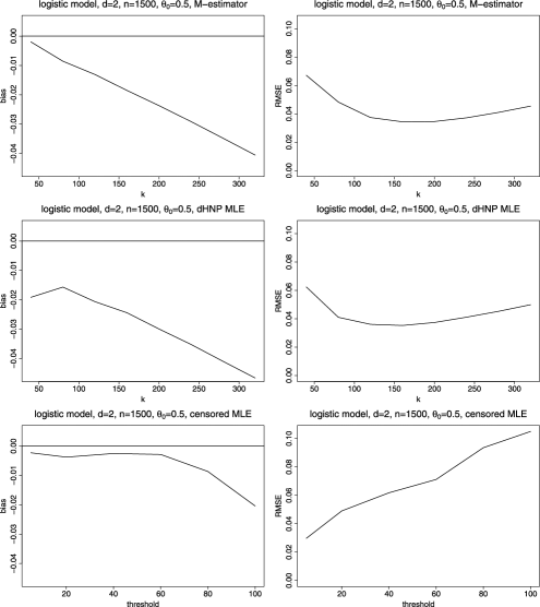
Figure 2: The M-estimator with $g(x,y)=g_{0}(x,y)=1$, the MLE from de Haan, Neves and Peng (2008) and the censored MLE, $d=2$.

$10$ and $160$, approximately, which amounts to thresholds between $5$ and $100$. This way we observe all estimators for their best region of thresholds. In Figure 2 we see that the methods perform roughly the same, the RMSEs being of the same order. The lowest RMSE of the censored MLE ($0.030$) is slightly smaller than the lowest RMSE of the M-estimator ($0.034$) and the lowest RMSE of the dHNP estimator ($0.035$), but the M- and the dHNP estimators are much more robust to the choice of the threshold.

Further simulation results

We simulate $500$ samples of size $n=1500$ from a five-dimensional logistic distribution function with $\theta_{0}=0.5$. As suggested by the sensitivity analysis, we opt for $g\equiv 1$ when defining $\hat{\theta}_{n}$. The bias and the RMSE of this estimator are shown in the upper panels of Figure 3.

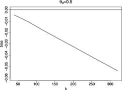
(a)	(b)
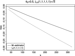
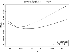
(c)	(d)

Figure 3: Logistic model, $d=5$, $\theta_{0}=0.5$, $l(1,1,1,1,1;\theta_{0})=\sqrt{5}$. (a) Bias of the M-estimator of $\theta$; (b) RMSE of the M-estimator of $\theta$; (c) bias of the estimators of $l(1,1,1,1,1;0.5)$; (d) RMSE of the estimators of $l(1,1,1,1,1;0.5)$.

Also, we consider the estimation of $l(1,1,1,1,1;\theta)$, based on this M-estimator $\hat{\theta}_{n}$. From (23) it follows that $l(1,1,1,1,1;\theta)=5^{\theta}$. The estimator of this quantity is then $5^{\hat{\theta}_{n}}$. Since $\theta_{0}=0.5$, the true parameter is $\sqrt{5}$. We compare the bias and the RMSE of this estimator and of the nonparametric estimator $\hat{l}_{n}(1,1,1,1,1)$; see (3). The lower panels in Figure 3 show that the M-estimator performs better than the nonparametric estimator for almost every $k$.

Real data: Testing and estimation

We use the bivariate Loss-ALAE data set, consisting of 1500 insurance claims, comprising losses and allocated loss adjustment expenses; for more information, see Frees and Valdez (1998). The scatterplots of the data and their joint ranks are shown in Figure 4. We consider the asymmetric logistic model described below for their tail dependence function and we test whether a more restrictive, symmetric logistic model suffices to describe the tail dependence of these data.

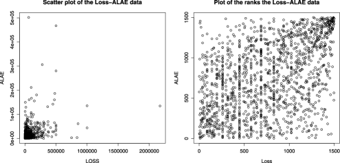
Figure 4: The insurance claims Loss-ALAE data.

The asymmetric logistic tail dependence function was introduced in Tawn (1988) as an extension of the logistic model. In dimension $d=2$ it is given by

$$\qquad l(x,y;\theta,\psi_{1},\psi_{2})=(1-\psi_{1})x+(1-\psi_{2})y+\bigl{(}(\psi_{1}x)^{1/\theta}+(\psi_{2}y)^{1/\theta}\bigr{)}^{\theta}$$ (24)

with the dependence parameter $\theta\in[0,1]$ and the asymmetry parameters $\psi_{1},\psi_{2}\in[0,1]$. This model yields a spectral measure $H$ with atoms at $(1,0)$ and $(0,1)$ whenever $\psi_{1}<1$ and $\psi_{2}<1$. When $\psi_{1}=\psi_{2}=:\psi$, we have the symmetric tail dependence function

$$l(x,y;\theta,\psi)=(1-\psi)(x+y)+\psi\bigl{(}x^{1/\theta}+y^{1/\theta}\bigr{)}^{\theta}.$$ (25)

For the given data, we test whether the use of this symmetric model is justified, as opposed to the wider asymmetric logistic model. Setting $\eta_{1}:=(\psi_{1}+\psi_{2})/2\in[0,1]$ and $\eta_{2}:=(\psi_{1}-\psi_{2})/2\in[-1/2,1/2]$, we reparametrize the model in (24) so that testing for symmetry amounts to testing whether $\eta_{2}=0$. By Corollary 4.4, the test statistic is given by

$$S_{n}:=\frac{k\hat{\eta}_{2}^{2}}{M_{2}(\hat{\theta},\hat{\eta}_{1},0)}.$$

Table 1 below shows the obtained values of $S_{n}$ for the Loss-ALAE data for selected values of $k$.

=310pt $k$ $50$ $100$ $150$ $200$ $250$ $S_{n}$ $0.041$ $0.139$ $0.294$ $0.477$ $0.681$

Table 1: Values of the test statistic $S_{n}$ for the Loss-ALAE data for selected values of $k$

Since the critical value is $3.84$, the null hypothesis is clearly not rejected. Hence, we adopt the symmetric tail dependence model (25) and we compute the M-estimates of $(\theta,\eta_{1})=(\theta,\psi)$, the auxiliary functions being $g_{1}(x,y)=x$ and $g_{2}(x,y)=2(x+y)$. For $k=150$, we obtain $(\hat{\theta},\hat{\psi})=(0.65,0.95)$ with estimated standard errors $0.032$ for $\hat{\theta}$ and $0.014$ for $\hat{\psi}$.

6 Example 2: Factor model

Consider the $r$-factor model, $r\in{\mathbb{N}}$, in dimension $d$: $X^{\prime}=(X_{1}^{\prime},\ldots,X_{d}^{\prime})$ and

$$X_{j}^{\prime}=\sum_{i=1}^{r}a_{ij}Z_{i}+\varepsilon_{j},\qquad j\in\{1,\ldots,d\},$$ (26)

with $Z_{i}$ independent Fréchet($\nu$) random variables, $\nu>0$, with $\varepsilon_{j}$ independent random variables which have a lighter right tail than the factors and are independent of them, and with $a_{ij}$ nonnegative constants such that $\sum_{j}a_{ij}>0$ for all $i$. Factor models of this type are common in various applications; for example, in finance, see Fama and French (1993), Malevergne and Sornette (2004), Geluk, de Haan and de Vries (2007). However, for the purpose of studying the tail properties, it is more convenient to consider the (max) factor model: $X=(X_{1},\ldots,X_{d})$ and

$$X_{j}=\max_{i=1,\ldots,r}\{a_{ij}Z_{i}\},\qquad j\in\{1,\ldots,d\},$$ (27)

with $a_{ij}$ and $Z_{i}$ as above. Note that $X^{\prime}$ and $X$ have the same tail dependence function $l$; this essentially follows from the fact that the ratio of the probabilities of the sum and the maximum of the $a_{ij}Z_{i}$ exceeding $x$ tends to 1 as $x\to\infty$ [Embrechts, Klüppelberg and Mikosch (1997), page 38]. Let $W_{i}=Z_{i}^{\nu}$, $i=1,\ldots,r$, and observe that the $W_{i}$ are standard Fréchet random variables. Define a $d$-dimensional random vector $Y=(Y_{1},\ldots,Y_{d})$ by

$$Y_{j}:=X_{j}^{\nu}=\max_{i=1,\ldots,r}\bigl{\{}a_{ij}^{\nu}W_{i}\bigr{\}},\qquad j\in\{1,\ldots,d\}.$$

It is easily seen that, as $x\to\infty$,

$$1-F_{Y_{j}}(x)=1-\exp\biggl{\{}-\frac{\sum_{i=1}^{r}a_{ij}^{\nu}}{x}\biggr{\}}\sim\frac{\sum_{i=1}^{r}a_{ij}^{\nu}}{x}.$$

Since the $X_{j}$ variables are increasing transformations of the $Y_{j}$ variables, the (tail) dependence structures of $X$ and $Y$ coincide. We will determine the tail dependence function $l$ and the spectral measure $H$ of $X$.

Lemma 6.1

Let $X$ follow a factor model given by (26) or (27). Then its stable tail dependence function is given by

$$l(x_{1},\ldots,x_{d})=\sum_{i=1}^{r}\max_{j=1,\ldots,d}\{b_{ij}x_{j}\},\qquad(x_{1},\ldots,x_{d})\in[0,\infty)^{d},$$ (28)

where $b_{ij}:=a_{ij}^{\nu}/\sum_{i=1}^{r}a_{ij}^{\nu}$.

Next, we are looking for a measure $H$ on the unit simplex $\Delta_{d-1}=\{w\in[0,\infty)^{d}\dvtx w_{1}+\cdots+w_{d}=1\}$ such that for all $x\in[0,\infty)^{d}$,

$$\sum_{i=1}^{r}\max_{j=1,\ldots,d}\{b_{ij}x_{j}\}=l(x_{1},\ldots,x_{d})=\int_{\Delta_{d-1}}\max_{j=1,\ldots,d}\{w_{j}x_{j}\}H(\mathrm{d}w).$$

This $H$ is a discrete measure with $r$ atoms given by

$$\biggl{(}\frac{b_{i1}}{\sum_{j}b_{ij}},\ldots,\frac{b_{id}}{\sum_{j}b_{ij}}\biggr{)},\qquad i\in\{1,\ldots,r\},$$ (29)

the atom receiving mass $\sum_{j}b_{ij}$, which is positive by assumption. Such measure $H$ is indeed a spectral measure, for

$$\int_{\Delta_{d-1}}w_{j}H(\mathrm{d}w)=\sum_{i=1}^{r}b_{ij}=1,\qquad j\in\{1,\ldots,d\}.$$ (30)

Every discrete spectral measure can arise in this way. This model for tail dependence is considered also in Ledford and Tawn (1998). Extensions to random fields are considered, for instance, in Wang and Stoev (2011).

The spectral measure is completely determined by the $r\times d$ parameters $b_{ij}$, but by the $d$ moment conditions from (30), the actual number of parameters is $p=(r-1)d$. The parameter vector $\theta\in{\mathbb{R}}^{p}$, which is to be estimated, can be constructed in many ways. For identification purposes, the definition of $\theta$ should be unambiguous. We opt for the following approach. Consider the matrix of the coefficients $b_{ij}$,

$$\left(\begin{array}[]{ccc}b_{11}&\cdots&b_{r1}\\ \vdots&\ddots&\vdots\\ b_{1d}&\cdots&b_{rd}\end{array}\right)\in{\mathbb{R}}^{d\times r}.$$

The coefficients corresponding to the $i$th factor, $i=1,\ldots,r$, are in the $i$th column of this matrix. We define $\theta$ by stacking the above columns in decreasing order of their sums, leaving out the column with the lowest sum. (If two columns have the same sum, we order them then in decreasing order lexicographically.)

The definition of the M-estimator of $\theta$ involves integrals of the form

$$\int_{[0,1]^{d}}g_{m}(x)l(x)\,\mathrm{d}x=\sum_{i=1}^{r}\int_{[0,1]^{d}}g_{m}(x)\max_{j=1,\ldots,d}\{b_{ij}x_{j}\}\,\mathrm{d}x,$$

where $g_{m}\dvtx[0,1]^{d}\to\mathbb{R}$ is integrable and $m=1,\ldots,q$. A possible choice is $g_{m}(x)=x_{k}^{s}$, where $k\in\{1,\ldots,d\}$ and $s\geq 0$.

Lemma 6.2

If $l$ is the tail dependence function of a factor model such that all $b_{ij}>0$, then

$$\int_{[0,1]^{d}}x_{k}^{s}l(x)\,\mathrm{d}x$$

$$\qquad=\sum_{i=1}^{r}\sum_{j=1}^{d}\frac{b_{ij}}{1+s(1-\delta_{jk})}\int_{0}^{1}\biggl{(}\frac{b_{ij}}{b_{ik}}x\wedge 1\biggr{)}^{s}\prod_{l=1}^{d}\biggl{(}\frac{b_{ij}}{b_{il}}x\wedge 1\biggr{)}\,\mathrm{d}x,$$

where $\delta_{jk}$ is $1$ if $j=k$ and $0$ if $j\neq k$.

We illustrate the performance of the M-estimator on two factor models: a four-dimensional model with $2$ factors ($p=1\times 4=4$), for simulated data sets, and a three-dimensional model with $3$ factors ($p=2\times 3=6$), for real financial data.

The integral on the right-hand side of (6.2) is to be computed numerically. For the factor model, the dependence of the matrix $M(\theta_{0})$ on $g$ is too complicated to obtain a general solution for the optimal function $g$. Since in the previous examples low degree polynomials gave very good results, and since by the previous lemma such a choice simplifies the calculations significantly (numerical integration in dimension $1$, instead of in dimension $d$), we considered such functions $g$ in a sensitivity analysis. It showed that the simplest cases give very good results in terms of root mean squared errors and that the performance of the M-estimator is quite robust to the particular choices of $g$. Hence, we suggest using simple, low degree polynomials for the functions $g$. The functions $g$ in the following examples are exactly of that type.

Simulation study: Four-dimensional model with two factors

We simulated $500$ samples of size $n=5000$ from a four-dimensional model:

$$X_{1} = 0.2Z_{1}\vee 0.8Z_{2},$$

$$X_{2} = 0.5Z_{1}\vee 0.5Z_{2},$$

$$X_{3} = 0.7Z_{1}\vee 0.3Z_{2},$$

$$X_{4} = 0.9Z_{1}\vee 0.1Z_{2}$$

with independent standard Fréchet factors $Z_{1}$ and $Z_{2}$. We have $\theta=(0.2,0.5,\break 0.7,0.9)$.

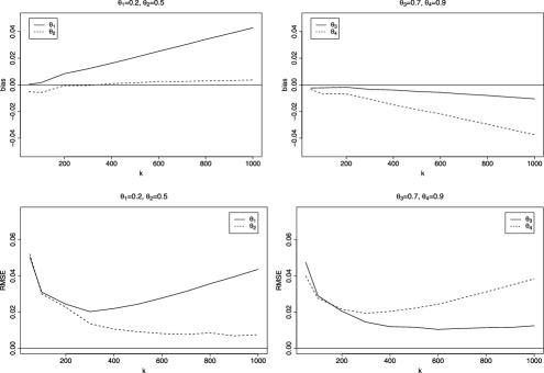
Figure 5: Four-dimensional 2-factor model, estimation of $\theta=(0.2,0.5,0.7,0.9)$.

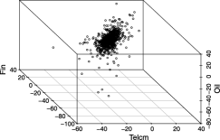
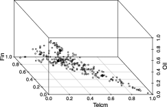
(a)	(b)

Figure 6: (a) Scatterplot of the original data; (b) plot of the pseudo-data and the three centers.

In Figure 5 we show the bias and the RMSE of the M-estimator based on $q=5$ moment equations, with auxiliary functions $g_{i}(x)=x_{i}$, for $i=1,2,3,4$ and $g_{5}\equiv 1$. The M-estimator performs very well. For relatively small $k$, the four components of $\theta$ are estimated equally well, whereas for larger $k$ the estimator performs somewhat better for parameter values in the “middle” of the interval $(0,1)$ than for values near $0$ or $1$.

Real data: Three-dimensional model with three factors

We considermonthly negative returns (losses) of three industry portfolios (Telecommunications, Finance and Oil) over the period July 1, 1926, until December 31, 2009. See Figure 6(a) for the scatterplot of the data; the sample size $n=1002$. The data are available at http://mba.tuck.dartmouth.edu/pages/ faculty/ken.french. We are interested in modeling the losses by a factor model. In the asset pricing literature [see, e.g., Fama and French (1993, 1996)], it is common to model the returns by linear factor models of type (26), with three underlying economic factors. Based on that line of literature, we also consider a three-factor model for the tails of the three industry portfolios above; see also Kleibergen (2011).

To estimate the parameter vector with $p=2\times 3=6$ components, we need to find a minimum of a 6-dimensional nonlinear criterion function. To solve such a difficult minimization problem, it is important to have good starting values. We find a starting parameter vector by applying the 3-means clustering algorithm [see, e.g., Pollard (1984), page 9] to the following pseudo-data: we transform the data (Telcm, Fin, Oil) to

$$\bigl{(}n/(n+1-R_{Ti}),n/(n+1-R_{Fi}),n/(n+1-R_{Oi})\bigr{)},\qquad i=1,\ldots,n,$$

where $R_{Ti}$, $R_{Fi}$ and $R_{Oi}$ are the ranks of the components of the $i$th observation. Only the entries such that the sum of their values is greater than the threshold $n/75$ are taken into account, and subsequently normalized so that they belong to the unit simplex $\Delta_{3-1}$; see Figure 6(b). We compute the 3-means cluster centers for these data. Using equation (29), we compute from these three centers the 6-dimensional starting parameter [as described below equation (30)] for the minimization routine. For the criterion function we use $q=7$ functions $g_{i}$ as follows: $g_{i}(x)=x_{i}$ for $i=1,2,3$, $g_{i}(x)=x_{i-3}^{2}$ for $i=4,5,6$, and $g_{7}\equiv 1$. For different choices of $k$, we obtain the estimates presented in Table 2. For each $k$, we estimate the loading of the first two factors. This corresponds to the first two columns of estimated ${b_{ij}}$ for each $k$. The third columns follow from the conditions in (30).

Table 2: Estimates for the factor loadings $b_{ij}$ in the three-factor model fitted to the tail of the Telcm/Fin/Oil data

$\bolds{k=60}$			$\bolds{k=90}$
$0.394$	$0.593$	$0.013$	$0.344$	$0.616$	$0.040$
$0.691$	$0.211$	$0.098$	$0.701$	$0.216$	$0.083$
$0.358$	$0.062$	$0.580$	$0.368$	$0.052$	$0.580$
$\bolds{k=120}$			$\bolds{k=150}$
$0.387$	$0.586$	$0.027$	$0.388$	$0.581$	$0.031$
$0.695$	$0.215$	$0.090$	$0.699$	$0.211$	$0.090$
$0.348$	$0.058$	$0.594$	$0.364$	$0.086$	$0.550$

Observe that the estimates do hardly depend on the choice of $k$. We see that all three portfolios load substantially on the first factor (the first column of estimated coefficients, for each $k$), but Telecommunications loads more on the second factor (the first lines of estimated coefficients), and Oil more on the third factor (the third lines of estimated coefficients). This indicates that even for only these three portfolios, three factors are required.

7 Proofs

The asymptotic properties of the nonparametric estimator $\hat{l}_{n}$ are required for the proofs of the asymptotic properties of the M-estimator $\hat{\theta}_{n}$. Consistency of $\hat{l}_{n}$ [see (32)] for dimension $d=2$ was shown in Huang (1992); cf. Drees and Huang (1998). In particular, it holds that for every $T>0$, as $n\to\infty$, $k\to\infty$ and $k/n\to 0$,

$$\sup_{(x_{1},x_{2})\in[0,T]^{2}}\bigl{|}\hat{l}_{n}(x_{1},x_{2})-l(x_{1},x_{2})\bigr{|}\stackrel{{\scriptstyle{\mathbb{P}}}}{{\to}}0.$$

The proof translates straightforwardly to general dimension $d$, and together with integrability of $g$ yields consistency of $\int g\hat{l}_{n}$ for $\int gl=\varphi(\theta_{0})$. For the proof of Theorem 4.1, a technical result is needed.

Let $\mathcal{H}_{k,n}(\theta)\in{\mathbb{R}}^{p\times p}$ denote the Hessian matrix of $Q_{k,n}$ as a function of $\theta$. Let $\mathcal{H}(\theta)$ be the deterministic, symmetric $p\times p$ matrix whose $(i,j)$th element, $i,j\in\{1,\ldots,p\}$, is equal to

$$\bigl{(}\mathcal{H}(\theta)\bigr{)}_{ij} = 2\biggl{(}\frac{\partial}{\partial\theta_{i}}\varphi(\theta)\biggr{)}^{T}\biggl{(}\frac{\partial}{\partial\theta_{j}}\varphi(\theta)\biggr{)}$$

$${}-2\biggl{(}\frac{\partial^{2}}{\partial\theta_{i}\,\partial\theta_{j}}\varphi(\theta)\biggr{)}^{T}\bigl{(}\varphi(\theta_{0})-\varphi(\theta)\bigr{)}.$$

Lemma 7.1

If $k/n\to 0$ and if the assumptions of Theorem 4.1(ii) are satisfied, then as $n\to\infty$ and $k\to\infty$, on some closed neighborhood of $\theta_{0}$, [(ii)]

$\mathcal{H}_{k,n}(\theta)\stackrel{{\scriptstyle{\mathbb{P}}}}{{\to}}\mathcal{H}(\theta)$ uniformly in $\theta$, and

${\mathbb{P}}(\mathcal{H}_{k,n}(\theta)\mbox{ is positive definite})\to 1$.

(i) The Hessian matrix of $Q_{k,n}$ in $\theta$ is a $p\times p$ matrix $\mathcal{H}_{k,n}(\theta)$ with elements $(\mathcal{H}_{k,n}(\theta))_{ij}=\partial^{2}Q_{k,n}(\theta)/\partial\theta_{j}\,\partial\theta_{i}$, for $i,j\in\{1,\ldots,p\}$, given by

$$\bigl{(}\mathcal{H}_{k,n}(\theta)\bigr{)}_{ij} = 2\sum_{m=1}^{q}\int_{[0,1]^{d}}g_{m}(x)\,\frac{\partial}{\partial\theta_{j}}l(x;\theta)\,\mathrm{d}x\cdot\int_{[0,1]^{d}}g_{m}(x)\,\frac{\partial}{\partial\theta_{i}}l(x;\theta)\,\mathrm{d}x$$

$${}-2\sum_{m=1}^{q}\int_{[0,1]^{d}}g_{m}(x)\,\frac{\partial^{2}}{\partial\theta_{j}\,\partial\theta_{i}}l(x;\theta)\,\mathrm{d}x$$

$$\hskip 36.2pt{}\times\int_{[0,1]^{d}}g_{m}(x)\bigl{(}\hat{l}_{n}(x)-l(x;\theta)\bigr{)}\,\mathrm{d}x$$

$$= 2\biggl{(}\frac{\partial}{\partial\theta_{i}}\varphi(\theta)\biggr{)}^{T}\biggl{(}\frac{\partial}{\partial\theta_{j}}\varphi(\theta)\biggr{)}-2\biggl{(}\frac{\partial^{2}}{\partial\theta_{i}\,\partial\theta_{j}}\varphi(\theta)\biggr{)}^{T}$$

$${}\times\biggl{(}\int_{[0,1]^{d}}g(x)\hat{l}_{n}(x)\,\mathrm{d}x-\varphi(\theta)\biggr{)}.$$

The consistency of $\int g\hat{l}_{n}$ for $\varphi(\theta_{0})$ implies

$$\bigl{(}\mathcal{H}_{k,n}(\theta)\bigr{)}_{ij} \stackrel{{\scriptstyle{\mathbb{P}}}}{{\to}} 2\biggl{(}\frac{\partial}{\partial\theta_{i}}\varphi(\theta)\biggr{)}^{T}\biggl{(}\frac{\partial}{\partial\theta_{j}}\varphi(\theta)\biggr{)}$$

$${}-2\biggl{(}\frac{\partial^{2}}{\partial\theta_{i}\,\partial\theta_{j}}\varphi(\theta)\biggr{)}^{T}\bigl{(}\varphi(\theta_{0})-\varphi(\theta)\bigr{)}$$

$$= \bigl{(}\mathcal{H}(\theta)\bigr{)}_{ij}.$$

Since we assumed that there exists $\varepsilon_{0}>0$ such that the set $\{\theta\in\Theta\dvtx\|\theta-\theta_{0}\|\leq\varepsilon_{0}\}=:B_{\varepsilon_{0}}(\theta_{0})$ is closed and thus compact, and since $\varphi$ is assumed to be twice continuously differentiable, the second derivatives of $\varphi$ are uniformly bounded on $B_{\varepsilon_{0}}(\theta_{0})$ and, hence, the convergence above is uniform on $B_{\varepsilon_{0}}(\theta_{0})$.

(ii) For $\theta=\theta_{0}$ we get

$$\bigl{(}\mathcal{H}(\theta_{0})\bigr{)}_{ij}=2\biggl{(}\frac{\partial}{\partial\theta_{i}}\varphi(\theta)\bigg{|}_{\theta=\theta_{0}}\biggr{)}^{T}\biggl{(}\frac{\partial}{\partial\theta_{j}}\varphi(\theta)\bigg{|}_{\theta=\theta_{0}}\biggr{)},$$

that is,

$$\mathcal{H}(\theta_{0})=2\dot{\varphi}(\theta_{0})^{T}\dot{\varphi}(\theta_{0}).$$

Since $\dot{\varphi}(\theta_{0})$ is assumed to be of full rank, $\mathcal{H}(\theta_{0})$ is positive definite. For $\theta$ close to $\theta_{0}$, $\mathcal{H}(\theta)$ is also positive definite. Due to the uniform convergence of $\mathcal{H}_{k,n}(\theta)$ to $\mathcal{H}(\theta)$ on $B_{\varepsilon_{0}}(\theta_{0})$, the matrix $\mathcal{H}_{k,n}(\theta)$ is also positive definite on $B_{\varepsilon_{0}}(\theta_{0})$ with probability tending to one.

Proof of Theorem 4.1 (i) Fix $\varepsilon>0$ such that $0<\varepsilon\leq\varepsilon_{0}$. Since $\varphi$ is a homeomorphism, there exists $\delta>0$ such that $\theta\in\Theta$ and $\|\varphi(\theta)-\varphi(\theta_{0})\|\leq\delta$ implies $\|\theta-\theta_{0}\|\leq\varepsilon$. In other words, for every $\theta\in\Theta$ such that $\|\theta-\theta_{0}\|>\varepsilon$, we have $\|\varphi(\theta)-\varphi(\theta_{0})\|>\delta$. Hence, on the event

$$A_{n}=\biggl{\{}\biggl{\|}\varphi(\theta_{0})-\int g\hat{l}_{n}\biggr{\|}\leq\delta/2\biggr{\}}$$

for every $\theta\in\Theta$ with $\|\theta-\theta_{0}\|>\varepsilon$, necessarily,

$$\biggl{\|}\varphi(\theta)-\int g\hat{l}_{n}\biggr{\|} \geq \bigl{\|}\varphi(\theta)-\varphi(\theta_{0})\bigr{\|}-\biggl{\|}\varphi(\theta_{0})-\int g\hat{l}_{n}\biggr{\|}$$

$$> \delta-\delta/2=\delta/2\geq\biggl{\|}\varphi(\theta_{0})-\int g\hat{l}_{n}\biggr{\|}.$$

As a consequence, on the event $A_{n}$, we have

$$\inf_{\theta\dvtx\|\theta-\theta_{0}\|>\varepsilon}\biggl{\|}\varphi(\theta)-\int g\hat{l}_{n}\biggr{\|}>\min_{\theta\dvtx\|\theta-\theta_{0}\|\leq\varepsilon}\biggl{\|}\varphi(\theta)-\int g\hat{l}_{n}\biggr{\|},$$

where we can write the minimum on the right-hand side since the set $\{\theta\in\Theta\dvtx\|\theta-\theta_{0}\|\leq\varepsilon\}$ is closed and thus compact for $0\leq\varepsilon\leq\varepsilon_{0}$. Hence, on the event $A_{n}$, the “argmin” set $\hat{\Theta}_{n}$ is nonempty and is contained in the closed ball of radius $\varepsilon$ centered at $\theta_{0}$. Finally, ${\mathbb{P}}(A_{n})\to 1$ by weak consistency of $\int g\hat{l}_{n}$ for $\int gl=\varphi(\theta_{0})$.

(ii) In the proof of (i) we have seen that, with probability tending to one, the proposed M-estimator exists and it is contained in a closed ball around $\theta_{0}$. In Lemma 7.1 we have shown that the criterion function is, with probability tending to one, strictly convex on such a closed ball around $\theta_{0}$ and, hence, with probability tending to one, the minimizer of the criterion function is unique.

For $i=1,\ldots,n$ let

$$U_{i}:=(U_{i1},\ldots,U_{id}):=\bigl{(}1-F_{1}(X_{i1}),\ldots,1-F_{d}(X_{id})\bigr{)}$$

and denote

$$Q_{nj}(u_{j}) := U_{\lceil nu_{j}\rceil\dvtx n,j},\qquad j=1,\ldots,d,$$

$$S_{nj}(x_{j}) := \frac{n}{k}Q_{nj}\biggl{(}\frac{kx_{j}}{n}\biggr{)},\qquad j=1,\ldots,d,$$

$$S_{n}(x) := \bigl{(}S_{n1}(x_{1}),\ldots,S_{nd}(x_{d})\bigr{)},$$

where $U_{1\dvtx n,j}\!\leq\!\cdots\!\leq\!U_{n\dvtx n,j}$ are the order statistics of $U_{1j},\ldots,U_{nj}$, $j\!=\!1,\ldots,d$, and $\lceil a\rceil$ is the smallest integer not smaller than $a$. Write

$$V_{n}(x):\! = \frac{n}{k}{\mathbb{P}}\biggl{(}U_{11}\leq\frac{kx_{1}}{n}\mbox{ or }\ldots\mbox{ or }U_{1d}\leq\frac{kx_{d}}{n}\biggr{)},$$

$$T_{n}(x):\! = \frac{1}{k}\sum_{i=1}^{n}\mathbf{1}\biggl{\{}U_{i1}<\frac{kx_{1}}{n}\mbox{ or }\ldots\mbox{ or }U_{id}<\frac{kx_{d}}{n}\biggr{\}},$$

$$\hat{L}_{n}(x):\! = \frac{1}{k}\sum_{i=1}^{n}\mathbf{1}\biggl{\{}U_{i1}<\frac{k}{n}S_{n1}(x_{1})\mbox{ or }\ldots\mbox{ or }U_{id}<\frac{k}{n}S_{nd}(x_{d})\biggr{\}}$$

$$= \frac{1}{k}\sum_{i=1}^{n}\mathbf{1}\bigl{\{}R_{i}^{1}>n+1-kx_{1}\mbox{ or }\ldots\mbox{ or }R_{i}^{d}>n+1-kx_{d}\bigr{\}}$$

and note that

$$\hat{L}_{n}(x)=T_{n}\bigl{(}S_{n}(x)\bigr{)}.$$

With probability one, for every $x$ and for every $j\in\{1,\ldots,d\}$, there is at most one $i$ such that $n+\frac{1}{2}-kx_{j}<R_{i}^{j}\leq n+1-kx_{j}$. Hence,

$$\sup_{x\in[0,1]^{d}}\sqrt{k}\bigl{|}\hat{l}_{n}(x)-\hat{L}_{n}(x)\bigr{|}\leq\frac{d}{\sqrt{k}}\to 0.$$ (32)

This shows that the asymptotic properties of $\hat{l}_{n}$ and $\hat{L}_{n}$ are the same. With the notation $v_{n}(x)=\sqrt{k}(T_{n}(x)-V_{n}(x))$, we have the following result.

Proposition 7.2

Let $T>0$ and denote $A_{x}:=\{u\in[0,\infty]^{d}\dvtx u_{1}\leq x_{1}$ or $\ldots$ or $u_{d}\leq x_{d}\}$. There exists a sequence of processes $\tilde{v}_{n}$ such that, for all $n$, $\tilde{v}_{n}\stackrel{{\scriptstyle d}}{{=}}v_{n}$ and there exists a Wiener process $W_{l}(x):=W_{\Lambda}(A_{x})$ such that as $n\to\infty$,

$$\sup_{x\in[0,2T]^{d}}\bigl{|}\tilde{v}_{n}(x)-W_{l}(x)\bigr{|}\stackrel{{\scriptstyle{\mathbb{P}}}}{{\to}}0.$$ (33)

The result follows from Theorem 3.1 in Einmahl (1997). From the proofs there it follows that a single Wiener process, instead of the sequence in the original statement of the theorem, can be used, and that convergence holds almost surely, instead of in probability, once the Skorohod construction is introduced. From now on, we work on this new (Skorohod) probability space, but keep the old notation, without the tildes. In particular, we have convergence of the marginal processes:

$$\sup_{x_{j}\in[0,2T]}\bigl{|}v_{nj}(x)-W_{l,j}(x_{j})\bigr{|}\to 0\qquad\mbox{a.s.},\qquad j=1,\ldots,d,$$

where $v_{nj}(x_{j}):=v_{n}((0,\ldots,0,x_{j},0,\ldots,0))$. The Vervaat (1972) lemma implies

$$\sup_{x_{j}\in[0,2T]}\bigl{|}\sqrt{k}\bigl{(}S_{nj}(x_{j})-x_{j}\bigr{)}+W_{l,j}(x_{j})\bigr{|}\to 0\qquad\mbox{a.s.},\qquad j=1,\ldots,d.$$ (34)

Proof of Theorem 4.6 Write

$$\sqrt{k}\bigl{(}\hat{L}_{n}(x)-l(x)\bigr{)}$$

$$\qquad=\sqrt{k}\bigl{(}T_{n}\bigl{(}S_{n}(x)\bigr{)}-V_{n}\bigl{(}S_{n}(x)\bigr{)}\bigr{)}+\sqrt{k}\bigl{(}V_{n}\bigl{(}S_{n}(x)\bigr{)}-l\bigl{(}S_{n}(x)\bigr{)}\bigr{)}$$

$$\qquad\quad{}+\sqrt{k}\bigl{(}l\bigl{(}S_{n}(x)\bigr{)}-l(x)\bigr{)}$$

$$\qquad=:D_{1}(x)+D_{2}(x)+D_{3}(x).$$

Proof of $\sup_{x\in[0,T]^{d}}|D_{1}(x)-W_{l}(x)|\stackrel{{\scriptstyle{\mathbb{P}}}}{{\to}}0$. We have

$$D_{1}(x)=\sqrt{k}\bigl{(}T_{n}\bigl{(}S_{n}(x)\bigr{)}-V_{n}\bigl{(}S_{n}(x)\bigr{)}\bigr{)}=v_{n}\bigl{(}S_{n}(x)\bigr{)}.$$

It holds that

$$\sup_{x\in[0,T]^{d}}\bigl{|}D_{1}(x)-W_{l}(x)\bigr{|}$$

$$\qquad\leq\sup_{x\in[0,T]^{d}}\bigl{|}D_{1}(x)-W_{l}\bigl{(}S_{n}(x)\bigr{)}\bigr{|}$$

$$\qquad\quad{}+\sup_{x\in[0,T]^{d}}\bigl{|}W_{l}\bigl{(}S_{n}(x)\bigr{)}-W_{l}(x)\bigr{|}.$$

Because of (34), this is, with probability tending to one, less than or equal to

$$\sup_{y\in[0,2T]^{d}}\bigl{|}v_{n}(y)-W_{l}(y)\bigr{|}+\sup_{x\in[0,T]^{d}}\bigl{|}W_{l}\bigl{(}S_{n}(x)\bigr{)}-W_{l}(x)\bigr{|}.$$

Both terms tend to zero in probability, the first one by Proposition 7.2, the second one because of the uniform continuity of $W_{l}$ and (34).

Proof of $\sup_{x\in[0,T]^{d}}|D_{2}(x)|\stackrel{{\scriptstyle{\mathbb{P}}}}{{\to}}0$.  Because of (34), with probability tending to one, $\sup_{x\in[0,T]^{d}}|D_{2}(x)|$ is less than or equal to $\sup_{y\in[0,2T]^{d}}\sqrt{k}|V_{n}(y)-l(y)|$, which in turn, because of conditions (C1) and (C2), is equal to

$$\sqrt{k}O\biggl{(}\biggl{(}\frac{k}{n}\biggr{)}^{\alpha}\biggr{)}=O\biggl{(}\biggl{(}\frac{k}{n^{2\alpha/(1+2\alpha)}}\biggr{)}^{1/2+\alpha}\biggr{)}=o(1).$$

Proof of $\sup_{x\in[0,T]^{d}}|D_{3}(x)+\sum_{j=1}^{d}l_{j}(x)W_{l,j}(x_{j})|\stackrel{{\scriptstyle{\mathbb{P}}}}{{\to}}0$. Due to the existence of the first derivatives, we can use the mean value theorem to write

$$\frac{1}{\sqrt{k}}D_{3}(x)=l\bigl{(}S_{n}(x)\bigr{)}-l(x)=\sum_{j=1}^{d}\bigl{(}S_{nj}(x_{j})-x_{j}\bigr{)}\cdot l_{j}(\xi_{n})$$

with $\xi_{n}$ between $x$ and $S_{n}(x)$. Therefore,

$$\sup_{x\in[0,T]^{d}}\Biggl{|}D_{3}(x)+\sum_{j=1}^{d}l_{j}(x)W_{l,j}(x_{j})\Biggr{|}$$

$$\qquad\leq\sum_{j=1}^{d}\bigl{|}l_{j}(\xi_{n})\sqrt{k}\bigl{(}S_{nj}(x_{j})-x_{j}\bigr{)}+l_{j}(x)W_{l,j}(x_{j})\bigr{|}.$$

Note that all the terms on the right-hand side of the above inequality can be dealt with in the same way. Therefore, we consider only the first term. For $\delta\in(0,T)$, this term is bounded by

$$\sup_{x\in[0,T]^{d}}\bigl{|}l_{1}(\xi_{n})\bigr{|}\cdot\sup_{x_{1}\in[0,T]}\bigl{|}\sqrt{k}\bigl{(}S_{n1}(x_{1})-x_{1}\bigr{)}+W_{(l,1)}(x_{1})\bigr{|}$$

$$\quad{}+\sup_{x\in[\delta,T]\times[0,T]^{d-1}}\bigl{|}l_{1}(\xi_{n})-l_{1}(x)\bigr{|}\cdot\sup_{x_{1}\in[0,T]}\bigl{|}W_{(l,1)}(x_{1})\bigr{|}$$

$$\quad{}+\sup_{x\in[0,\delta]\times[0,T]^{d-1}}\bigl{|}l_{1}(\xi_{n})-l_{1}(x)\bigr{|}\cdot\sup_{x_{1}\in[0,\delta]}\bigl{|}W_{(l,1)}(x_{1})\bigr{|}$$

$$\qquad=:D_{4}\cdot D_{5}+D_{6}\cdot D_{7}+D_{8}\cdot D_{9}.$$

Observe that $0\leq l_{1}\leq 1$. Also, since $l_{1}$ is continuous on $[\delta/2,T]\times[0,T]^{d-1}$, it is uniformly continuous on that region. We have $D_{5}\stackrel{{\scriptstyle{\mathbb{P}}}}{{\to}}0$ by (34), so $D_{4}\cdot D_{5}\stackrel{{\scriptstyle{\mathbb{P}}}}{{\to}}0$. The uniform continuity of $l_{1}$ and the fact that almost surely $D_{7}<\infty$ yield $D_{6}\cdot D_{7}\stackrel{{\scriptstyle{\mathbb{P}}}}{{\to}}0$. Finally, for every $\varepsilon>0$, we can find a $\delta$ such that, with probability at least $1-\varepsilon$, $D_{9}<\varepsilon$ and, hence, $D_{8}\cdot D_{9}<\varepsilon$.

Applying (32) completes the proof.

Proposition 7.3

If conditions (C1) and (C2) from Theorem 4.2 hold, then as $n\to\infty$,

$$\sqrt{k}\int_{[0,1]^{d}}g(x)\bigl{(}\hat{l}_{n}(x)-l(x)\bigr{)}\,\mathrm{d}x\stackrel{{\scriptstyle d}}{{\to}}\tilde{B}.$$ (35)

Throughout the proof we write $l(x)$ instead of $l(x;\theta_{0})$. Also, since $l$ does not need to be differentiable, we will use notation $l_{j}(x)$, $j=1,\ldots,d$, to denote the right-hand partial derivatives here. Let $D_{1}(x),D_{2}(x),\break D_{3}(x)$ be as in the proof of Theorem 4.6 and take $T=1$. Then

$$\biggl{|}\sqrt{k}\biggl{(}\int_{[0,1]^{d}}g(x)\hat{L}_{n}(x)\,\mathrm{d}x-\int_{[0,1]^{d}}g(x)l(x)\,\mathrm{d}x\biggr{)}-\tilde{B}\biggr{|}$$

$$\qquad\leq\sup_{x\in[0,1]^{d}}\bigl{|}D_{1}(x)-W_{l}(x)\bigr{|}\int_{[0,1]^{d}}\bigl{|}g(x)\bigr{|}\,\mathrm{d}x+\sup_{x\in[0,1]^{d}}\bigl{|}D_{2}(x)\bigr{|}\int_{[0,1]^{d}}\bigl{|}g(x)\bigr{|}\,\mathrm{d}x$$

$$\qquad\quad{}+\int_{[0,1]^{d}}\bigl{|}g(x,y)\bigr{|}\cdot\Biggl{|}D_{3}(x)+\sum_{j=1}^{d}l_{j}(x)W_{l,j}(x_{j})\Biggr{|}\,\mathrm{d}x.$$

The first two terms on the right-hand side converge to zero in probability due to integrability of $g$ and uniform convergence of $D_{1}(x)$ and $D_{2}(x)$, which was shown in the proof of Theorem 4.6. The third term needs to be treated separately, as the condition on continuity (and existence) of partial derivatives is no longer assumed to hold.

Let $\omega$ be a point in the Skorohod probability space introduced before the proof of Theorem 4.6 such that for all $j=1,\ldots,d$,

$$\sup_{x_{j}\in[0,1]}\bigl{|}W_{l,j}(x_{j})\bigr{|}<+\infty\quad\mbox{and}\quad\sup_{x_{j}\in[0,1]}\bigl{|}\sqrt{k}\bigl{(}S_{nj}(x_{j})-x_{j}\bigr{)}+W_{l,j}(x_{j})\bigr{|}\to 0.$$

For such $\omega$ we will show by means of dominated convergence that

$$\quad\int_{[0,1]^{d}}\bigl{|}g(x)\bigr{|}\cdot\Biggl{|}\sqrt{k}\bigl{(}l\bigl{(}S_{n}(x)\bigr{)}-l(x)\bigr{)}+\sum_{j=1}^{d}l_{j}(x)W_{l,j}(x_{j})\Biggr{|}\,\mathrm{d}x\to 0.$$ (36)

Proof of the pointwise convergence. If $l$ is differentiable, convergence of the above integrand to zero follows from the definition of partial derivatives and (34). Since this might fail only on a set of Lebesgue measure zero, the convergence of the integrand to zero holds almost everywhere on $[0,1]^{d}$.

Proof of the domination. Note that from expressions for (one-sided) partial derivatives (2), and the moment conditions (4), it follows that $0\leq l_{j}(x)\leq 1$, for all $x\in[0,1]^{d}$ and all $j=1,\ldots,d$.

We get

$$\bigl{|}g(x)\bigr{|}\cdot\Biggl{|}\sqrt{k}\bigl{(}l\bigl{(}S_{n}(x)\bigr{)}-l(x)\bigr{)}+\sum_{j=1}^{d}l_{j}(x)W_{l,j}(x_{j})\Biggr{|}$$

$$\qquad\leq\bigl{|}g(x)\bigr{|}\cdot\Biggl{(}\sqrt{k}\bigl{|}l\bigl{(}S_{n}(x)\bigr{)}-l(x)\bigr{|}+\sum_{j=1}^{d}\bigl{|}W_{l,j}(x_{j})\bigr{|}\Biggr{)}.$$

Using the definition of function $l$ and uniformity of $1-F_{j}(X_{1j})$, we have, for all $j=1,\ldots,d$,

$$\bigl{|}l(x_{1},\ldots,x_{j-1},x_{j},x_{j+1},\ldots,x_{d})-l\bigl{(}x_{1},\ldots,x_{j-1},x_{j}^{\prime},x_{j+1},\ldots,x_{d}\bigr{)}\bigr{|}\leq\bigl{|}x_{j}-x_{j}^{\prime}\bigr{|}.$$

Hence, we can write

$$\sup_{x\in[0,1]^{d}}\sqrt{k}\bigl{|}l\bigl{(}S_{n}(x)\bigr{)}-l(x)\bigr{|}$$

$$\qquad\leq\sup_{x\in[0,1]^{d}}\sqrt{k}\bigl{|}l\bigl{(}S_{n}(x)\bigr{)}-l\bigl{(}x_{1},S_{n2}(x_{2}),\ldots,S_{nd}(x_{d})\bigr{)}\bigr{|}$$

$$\qquad\quad{}+\sup_{x\in[0,1]^{d}}\sqrt{k}\bigl{|}l\bigl{(}x_{1},S_{n2}(x_{2}),S_{n3}(x_{3}),\ldots,S_{nd}(x_{d})\bigr{)}$$

$$\qquad\quad\hskip 74.0pt{}-l\bigl{(}x_{1},x_{2},S_{n3}(x_{3}),\ldots,S_{nd}(x_{d})\bigr{)}\bigr{|}+\cdots$$

$$\qquad\quad{}+\sup_{x\in[0,1]^{d}}\sqrt{k}\bigl{|}l\bigl{(}x_{1},\ldots,x_{d-1},S_{nd}(x_{d})\bigr{)}-l(x)\bigr{|}$$

$$\qquad\leq\sum_{j=1}^{d}\sup_{x_{j}\in[0,1]}\sqrt{k}\bigl{|}S_{nj}(x_{j})-x_{j}\bigr{|}=O(1).$$

Since for all $j=1,\ldots,d$ we have ${\sup_{x_{j}\in[0,1]}}|W_{l,j}(x_{j})|<+\infty$, the proof of (36) is complete. This, together with (32), finishes the proof of the proposition.

Let $\nabla Q_{k,n}(\theta)\in{\mathbb{R}}^{p\times 1}$ be the gradient vector of $Q_{k,n}$ at $\theta$. Put

$$V(\theta):=4\dot{\varphi}(\theta)^{T}\Sigma(\theta)\dot{\varphi}(\theta)\in{\mathbb{R}}^{p\times p}.$$

Lemma 7.4

If the assumptions of Theorem 4.2 are satisfied, then as $n\to\infty$,

$$\sqrt{k}\nabla Q_{k,n}(\theta_{0})\stackrel{{\scriptstyle d}}{{\to}}N\bigl{(}0,V(\theta_{0})\bigr{)}.$$

The gradient vector of $Q_{k,n}$ with respect to $\theta$ in $\theta_{0}$ is

$$\nabla Q_{k,n}(\theta_{0})=\biggl{(}\frac{\partial}{\partial\theta_{1}}Q_{k,n}(\theta)\bigg{|}_{\theta=\theta_{0}},\ldots,\frac{\partial}{\partial\theta_{p}}Q_{k,n}(\theta)\bigg{|}_{\theta=\theta_{0}}\biggr{)}^{T},$$

where for $i=1,\ldots,p$,

$$\frac{\partial}{\partial\theta_{i}}Q_{k,n}(\theta)\bigg{|}_{\theta=\theta_{0}}$$

$$\qquad=-2\sum_{m=1}^{q}\int_{[0,1]^{d}}g_{m}(x)\,\frac{\partial}{\partial\theta_{i}}l(x;\theta)\bigg{|}_{\theta=\theta_{0}}\,\mathrm{d}x$$

$$\qquad\quad{}\times\int_{[0,1]^{d}}g_{m}(x)\bigl{(}\hat{l}_{n}(x)-l(x;\theta_{0})\bigr{)}\,\mathrm{d}x.$$

Using vector notation, we obtain

$$\nabla Q_{k,n}(\theta_{0})=-2\dot{\varphi}(\theta_{0})^{T}\cdot\int_{[0,1]^{d}}g(x)\bigl{(}\hat{l}_{n}(x)-l(x;\theta_{0})\bigr{)}\,\mathrm{d}x.$$

Equation (32) and the proof of Proposition 7.3 imply that

$$\sqrt{k}\nabla Q_{k,n}(\theta_{0})=-2\dot{\varphi}(\theta_{0})^{T}\cdot\int_{[0,1]^{d}}g(x)\sqrt{k}\bigl{(}\hat{l}_{n}(x)-l(x;\theta_{0})\bigr{)}\,\mathrm{d}x\stackrel{{\scriptstyle d}}{{\to}}-2\dot{\varphi}(\theta_{0})^{T}\tilde{B}.$$

The limit distribution of $\sqrt{k}\nabla Q_{k,n}(\theta_{0})$ is therefore zero-mean Gaussian with covariance matrix $V(\theta_{0})=4\dot{\varphi}(\theta_{0})^{T}\Sigma(\theta_{0})\dot{\varphi}(\theta_{0})$.

Proof of Theorem 4.2 Consider the function $f(t):=\nabla Q_{k,n}(\theta_{0}+t(\hat{\theta}_{n}-\theta_{0}))$, $t\in[0,1]$. The mean value theorem yields

$$\nabla Q_{k,n}(\hat{\theta}_{n})=\nabla Q_{k,n}(\theta_{0})+\mathcal{H}_{k,n}(\tilde{\theta}_{n})(\hat{\theta}_{n}-\theta_{0})$$

for some $\tilde{\theta}_{n}$ between $\theta_{0}$ and $\hat{\theta}_{n}$. First note that, with probability tending to one, $0=\nabla Q_{k,n}(\hat{\theta}_{n})$, which follows from the fact that $\hat{\theta}_{n}$ is a minimizer of $Q_{k,n}$ and that, with probability tending to one, $\hat{\theta}_{n}$ is in an open ball around $\theta_{0}$. By the consistency of $\hat{\theta}_{n}$, we have that $\tilde{\theta}_{n}\stackrel{{\scriptstyle{\mathbb{P}}}}{{\to}}\theta_{0}$, and since the convergence of $\mathcal{H}_{k,n}$ to $\mathcal{H}$ is uniform on a neighborhood of $\theta_{0}$, we get that $\mathcal{H}_{k,n}(\tilde{\theta}_{n})\stackrel{{\scriptstyle{\mathbb{P}}}}{{\to}}\mathcal{H}(\theta_{0})$. Hence, $\sqrt{k}(\hat{\theta}_{n}-\theta_{0})\stackrel{{\scriptstyle d}}{{\to}}N(0,M(\theta_{0}))$.

Proof of Corollary 4.3 As in Lemma 7.2 in Einmahl, Krajina and Segers (2008), we can see that if $\theta\mapsto H_{\theta}$ is weakly continuous at $\theta_{0}$, then $\theta\mapsto\Sigma(\theta)$ is continuous at $\theta_{0}$. This, together with the assumption that $\varphi$ is twice continuously differentiable and $\dot{\varphi}(\theta_{0})$ is of full rank, yields that $\theta\mapsto V(\theta)$ is continuous at $\theta_{0}$. The above assumption also implies that $\theta\mapsto\mathcal{H}(\theta)$ is continuous at $\theta_{0}$, which, with the positive definiteness of $\mathcal{H}(\theta)$ in a neighborhood of $\theta_{0}$, shows that if $\theta\mapsto H_{\theta}$ is weakly continuous at $\theta_{0}$, then $\theta\mapsto M(\theta)=\mathcal{H}(\theta)^{-1}V(\theta)\mathcal{H}(\theta)^{-1}$ is continuous at $\theta_{0}$. Hence, we obtain

$$M(\hat{\theta}_{n})^{-1/2}\sqrt{k}(\hat{\theta}_{n}-\theta_{0})\stackrel{{\scriptstyle d}}{{\to}}N(0,I_{p}),$$

which yields (4.3).

Proof of Theorem 4.4 Theorem 4.2 and the arguments used in the proof of Corollary 4.3 imply that, as $n\to\infty$,

$$M_{2}^{-1/2}\bigl{(}\hat{\theta}_{1},\theta_{2}^{*}\bigr{)}\sqrt{k}\bigl{(}\hat{\theta}_{2}-\theta_{2}^{*}\bigr{)}\stackrel{{\scriptstyle d}}{{\to}}N(0,I_{r})$$ (37)

and hence (21).

Proof of Lemma 6.1 We have

$$l(x_{1},\ldots,x_{d}) = \lim_{t\to\infty}t{\mathbb{P}}\bigl{(}1-F_{1}(X_{1})\leq x_{1}/t\mbox{ or }\ldots\mbox{ or }1-F_{d}(X_{d})\leq x_{d}/t\bigr{)}$$

$$= \lim_{t\to\infty}t{\mathbb{P}}\bigl{(}1-F_{Y_{1}}(Y_{1})\leq x_{1}/t\mbox{ or }\ldots\mbox{ or }1-F_{Y_{d}}(Y_{d})\leq x_{d}/t\bigr{)}$$

$$= \lim_{t\to\infty}t{\mathbb{P}}\biggl{(}Y_{1}\geq\frac{t\sum_{i=1}^{r}a_{i1}^{\nu}}{x_{1}}\mbox{ or }\ldots\mbox{ or }Y_{d}\geq\frac{t\sum_{i=1}^{r}a_{id}^{\nu}}{x_{d}}\biggr{)}$$

$$= \lim_{t\to\infty}t{\mathbb{P}}\biggl{(}\bigcup_{1\leq j\leq d}\bigcup_{1\leq i\leq r}\biggl{\{}W_{i}\geq\frac{t\sum_{i=1}^{r}a_{ij}^{\nu}}{a_{ij}^{\nu}x_{j}}\biggr{\}}\biggr{)}$$

$$= \lim_{t\to\infty}t{\mathbb{P}}\biggl{(}\bigcup_{1\leq i\leq r}\biggl{\{}W_{i}\geq\min_{1\leq j\leq d}\frac{t\sum_{i=1}^{r}a_{ij}^{\nu}}{a_{ij}^{\nu}x_{j}}\biggr{\}}\biggr{)}$$

$$= \lim_{t\to\infty}t\sum_{i=1}^{r}{\mathbb{P}}\biggl{(}W_{i}\geq\min_{1\leq j\leq d}\frac{t\sum_{i=1}^{r}a_{ij}^{\nu}}{a_{ij}^{\nu}x_{j}}\biggr{)}$$

$$= \lim_{t\to\infty}\sum_{i=1}^{r}t\biggl{(}1-\exp\biggl{\{}-\frac{1}{t}\max_{1\leq j\leq d}\frac{a_{ij}^{\nu}x_{j}}{\sum_{i=1}^{r}a_{ij}^{\nu}}\biggr{\}}\biggr{)}$$

$$= \sum_{i=1}^{r}\max_{1\leq j\leq d}\biggl{\{}\frac{a_{ij}^{\nu}x_{j}}{\sum_{i=1}^{r}a_{ij}^{\nu}}\biggr{\}}=:\sum_{i=1}^{r}\max_{1\leq j\leq d}\{b_{ij}x_{j}\}$$

as required.

Proof of Lemma 6.2 Fix $i\in\{1,\ldots,r\}$. We have

$$\int_{[0,1]^{d}}x_{k}^{s}\max_{1\leq j\leq d}\{b_{ij}x_{j}\}\,\mathrm{d}x=\sum_{j=1}^{d}\int_{[0,1]^{d}}x_{k}^{s}(b_{ij}x_{j})\mathbf{1}\Bigl{(}b_{ij}x_{j}\geq\max_{l\neq j}\{b_{il}x_{l}\}\Bigr{)}\,\mathrm{d}x.$$

Write the integral as a double integral, the outer integral with respect to $x_{j}\in[0,1]$ and the inner integral with respect to $x_{-j}=(x_{l})_{l\neq j}\in\mathbb{R}^{d-1}$ over the relevant domain. We find

$$\int_{[0,1]^{d}}x_{k}^{s}\max_{1\leq j\leq d}\{b_{ij}x_{j}\}\,\mathrm{d}x=\sum_{j=1}^{d}\int_{0}^{1}b_{ij}x_{j}\int_{0<x_{l}<({b_{ij}}/{b_{il}})x_{j}\wedge 1}x_{k}^{s}\,\mathrm{d}x_{-j}\,\mathrm{d}x_{j}.$$

After some long, but elementary computations, this simplifies to the stated expression.

References

- Ballani and Schlather (2011) {barticle}[mr] \bauthor\bsnmBallani, \bfnmF.\binitsF. and \bauthor\bsnmSchlather, \bfnmM.\binitsM. (\byear2011). \btitleA construction principle for multivariate extreme value distributions. \bjournalBiometrika \bvolume98 \bpages633–645. \biddoi=10.1093/biomet/asr034, issn=0006-3444, mr=2836411 \bptokimsref \endbibitem
- Beirlant et al. (2004) {bbook}[mr] \bauthor\bsnmBeirlant, \bfnmJan\binitsJ., \bauthor\bsnmGoegebeur, \bfnmYuri\binitsY., \bauthor\bsnmTeugels, \bfnmJozef\binitsJ. and \bauthor\bsnmSegers, \bfnmJohan\binitsJ. (\byear2004). \btitleStatistics of Extremes: Theory and Applications. \bpublisherWiley, \baddressChichester. \biddoi=10.1002/0470012382, mr=2108013 \bptokimsref \endbibitem
- Boldi and Davison (2007) {barticle}[mr] \bauthor\bsnmBoldi, \bfnmM. O.\binitsM. O. and \bauthor\bsnmDavison, \bfnmA. C.\binitsA. C. (\byear2007). \btitleA mixture model for multivariate extremes. \bjournalJ. R. Stat. Soc. Ser. B Stat. Methodol. \bvolume69 \bpages217–229. \biddoi=10.1111/j.1467-9868.2007.00585.x, issn=1369-7412, mr=2325273 \bptokimsref \endbibitem
- Coles and Tawn (1991) {barticle}[mr] \bauthor\bsnmColes, \bfnmStuart G.\binitsS. G. and \bauthor\bsnmTawn, \bfnmJonathan A.\binitsJ. A. (\byear1991). \btitleModelling extreme multivariate events. \bjournalJ. R. Stat. Soc. Ser. B Stat. Methodol. \bvolume53 \bpages377–392. \bidissn=0035-9246, mr=1108334 \bptokimsref \endbibitem
- Cooley, Davis and Naveau (2010) {barticle}[mr] \bauthor\bsnmCooley, \bfnmDaniel\binitsD., \bauthor\bsnmDavis, \bfnmRichard A.\binitsR. A. and \bauthor\bsnmNaveau, \bfnmPhilippe\binitsP. (\byear2010). \btitleThe pairwise beta distribution: A flexible parametric multivariate model for extremes. \bjournalJ. Multivariate Anal. \bvolume101 \bpages2103–2117. \biddoi=10.1016/j.jmva.2010.04.007, issn=0047-259X, mr=2671204 \bptokimsref \endbibitem
- de Haan and Ferreira (2006) {bbook}[mr] \bauthor\bparticlede \bsnmHaan, \bfnmLaurens\binitsL. and \bauthor\bsnmFerreira, \bfnmAna\binitsA. (\byear2006). \btitleExtreme Value Theory: An Introduction. \bpublisherSpringer, \baddressNew York. \bidmr=2234156 \bptokimsref \endbibitem
- de Haan, Neves and Peng (2008) {barticle}[mr] \bauthor\bparticlede \bsnmHaan, \bfnmLaurens\binitsL., \bauthor\bsnmNeves, \bfnmCláudia\binitsC. and \bauthor\bsnmPeng, \bfnmLiang\binitsL. (\byear2008). \btitleParametric tail copula estimation and model testing. \bjournalJ. Multivariate Anal. \bvolume99 \bpages1260–1275. \biddoi=10.1016/j.jmva.2007.08.003, issn=0047-259X, mr=2419346 \bptokimsref \endbibitem
- de Haan and Resnick (1977) {barticle}[mr] \bauthor\bparticlede \bsnmHaan, \bfnmLaurens\binitsL. and \bauthor\bsnmResnick, \bfnmSidney I.\binitsS. I. (\byear1977). \btitleLimit theory for multivariate sample extremes. \bjournalZ. Wahrsch. Verw. Gebiete \bvolume40 \bpages317–337. \bidmr=0478290 \bptokimsref \endbibitem
- Drees and Huang (1998) {barticle}[mr] \bauthor\bsnmDrees, \bfnmHolger\binitsH. and \bauthor\bsnmHuang, \bfnmXin\binitsX. (\byear1998). \btitleBest attainable rates of convergence for estimators of the stable tail dependence function. \bjournalJ. Multivariate Anal. \bvolume64 \bpages25–47. \biddoi=10.1006/jmva.1997.1708, issn=0047-259X, mr=1619974 \bptokimsref \endbibitem
- Einmahl (1997) {barticle}[mr] \bauthor\bsnmEinmahl, \bfnmJohn H. J.\binitsJ. H. J. (\byear1997). \btitlePoisson and Gaussian approximation of weighted local empirical processes. \bjournalStochastic Process. Appl. \bvolume70 \bpages31–58. \biddoi=10.1016/S0304-4149(97)00055-0, issn=0304-4149, mr=1472958 \bptokimsref \endbibitem
- Einmahl, Krajina and Segers (2008) {barticle}[mr] \bauthor\bsnmEinmahl, \bfnmJohn H. J.\binitsJ. H. J., \bauthor\bsnmKrajina, \bfnmAndrea\binitsA. and \bauthor\bsnmSegers, \bfnmJohan\binitsJ. (\byear2008). \btitleA method of moments estimator of tail dependence. \bjournalBernoulli \bvolume14 \bpages1003–1026. \biddoi=10.3150/08-BEJ130, issn=1350-7265, mr=2543584 \bptokimsref \endbibitem
- Embrechts, Klüppelberg and Mikosch (1997) {bbook}[mr] \bauthor\bsnmEmbrechts, \bfnmPaul\binitsP., \bauthor\bsnmKlüppelberg, \bfnmClaudia\binitsC. and \bauthor\bsnmMikosch, \bfnmThomas\binitsT. (\byear1997). \btitleModelling Extremal Events for Insurance and Finance. \bseriesApplications of Mathematics (New York) \bvolume33. \bpublisherSpringer, \baddressBerlin. \bidmr=1458613 \bptokimsref \endbibitem
- Fama and French (1993) {barticle}[author] \bauthor\bsnmFama, \bfnmE. F.\binitsE. F. and \bauthor\bsnmFrench, \bfnmK. R.\binitsK. R. (\byear1993). \btitleCommon risk factors in the returns on stocks and bonds. \bjournalJournal of Financial Economics \bvolume33 \bpages3–56. \bptokimsref \endbibitem
- Fama and French (1996) {barticle}[author] \bauthor\bsnmFama, \bfnmE. F.\binitsE. F. and \bauthor\bsnmFrench, \bfnmK. R.\binitsK. R. (\byear1996). \btitleMultifactor explanations of asset pricing anomalies. \bjournalJ. Finance \bvolume51 \bpages55–84. \bptokimsref \endbibitem
- Frees and Valdez (1998) {barticle}[mr] \bauthor\bsnmFrees, \bfnmEdward W.\binitsE. W. and \bauthor\bsnmValdez, \bfnmEmiliano A.\binitsE. A. (\byear1998). \btitleUnderstanding relationships using copulas. \bjournalN. Am. Actuar. J. \bvolume2 \bpages1–25. \bidissn=1092-0277, mr=1988432 \bptokimsref \endbibitem
- Geluk, de Haan and de Vries (2007) {bmisc}[author] \bauthor\bsnmGeluk, \bfnmJ. L.\binitsJ. L., \bauthor\bparticlede \bsnmHaan, \bfnmL.\binitsL. and \bauthor\bparticlede \bsnmVries, \bfnmC. G.\binitsC. G. (\byear2007). \bhowpublishedWeak and strong financial fragility. Technical Report 2007-023/2, Tinbergen Institute. \bptokimsref \endbibitem
- Guillotte, Perron and Segers (2011) {barticle}[mr] \bauthor\bsnmGuillotte, \bfnmSimon\binitsS., \bauthor\bsnmPerron, \bfnmFrançois\binitsF. and \bauthor\bsnmSegers, \bfnmJohan\binitsJ. (\byear2011). \btitleNon-parametric Bayesian inference on bivariate extremes. \bjournalJ. R. Stat. Soc. Ser. B Stat. Methodol. \bvolume73 \bpages377–406. \biddoi=10.1111/j.1467-9868.2010.00770.x, issn=1369-7412, mr=2815781 \bptokimsref \endbibitem
- Gumbel (1960) {barticle}[mr] \bauthor\bsnmGumbel, \bfnmE. J.\binitsE. J. (\byear1960). \btitleBivariate exponential distributions. \bjournalJ. Amer. Statist. Assoc. \bvolume55 \bpages698–707. \bidissn=0162-1459, mr=0116403 \bptokimsref \endbibitem
- Huang (1992) {bmisc}[author] \bauthor\bsnmHuang, \bfnmX.\binitsX. (\byear1992). \bhowpublishedStatistics of bivariate extreme values. Ph.D. thesis, Tinbergen Institute Research Series. \bptokimsref \endbibitem
- Joe, Smith and Weissman (1992) {barticle}[mr] \bauthor\bsnmJoe, \bfnmHarry\binitsH., \bauthor\bsnmSmith, \bfnmRichard L.\binitsR. L. and \bauthor\bsnmWeissman, \bfnmIshay\binitsI. (\byear1992). \btitleBivariate threshold methods for extremes. \bjournalJ. R. Stat. Soc. Ser. B Stat. Methodol. \bvolume54 \bpages171–183. \bidissn=0035-9246, mr=1157718 \bptokimsref \endbibitem
- Kleibergen (2011) {bmisc}[author] \bauthor\bsnmKleibergen, \bfnmFrank\binitsF. (\byear2011). \bhowpublishedReality checks for and of factor pricing. Technical report, Dept. Economics, Brown Univ. Preprint. Available at http://www.econ.brown.edu/fac/ Frank_Kleibergen/. \bptokimsref \endbibitem
- Ledford and Tawn (1996) {barticle}[mr] \bauthor\bsnmLedford, \bfnmAnthony W.\binitsA. W. and \bauthor\bsnmTawn, \bfnmJonathan A.\binitsJ. A. (\byear1996). \btitleStatistics for near independence in multivariate extreme values. \bjournalBiometrika \bvolume83 \bpages169–187. \biddoi=10.1093/biomet/83.1.169, issn=0006-3444, mr=1399163 \bptokimsref \endbibitem
- Ledford and Tawn (1998) {barticle}[mr] \bauthor\bsnmLedford, \bfnmAnthony W.\binitsA. W. and \bauthor\bsnmTawn, \bfnmJonathan A.\binitsJ. A. (\byear1998). \btitleConcomitant tail behaviour for extremes. \bjournalAdv. in Appl. Probab. \bvolume30 \bpages197–215. \biddoi=10.1239/aap/1035228000, issn=0001-8678, mr=1618837 \bptokimsref \endbibitem
- Malevergne and Sornette (2004) {barticle}[author] \bauthor\bsnmMalevergne, \bfnmY.\binitsY. and \bauthor\bsnmSornette, \bfnmD.\binitsD. (\byear2004). \btitleTail dependence of factor models. \bjournalJournal of Risk \bvolume6 \bpages71–116. \bptokimsref \endbibitem
- Pollard (1984) {bbook}[mr] \bauthor\bsnmPollard, \bfnmDavid\binitsD. (\byear1984). \btitleConvergence of Stochastic Processes. \bpublisherSpringer, \baddressNew York. \biddoi=10.1007/978-1-4612-5254-2, mr=0762984 \bptokimsref \endbibitem
- Resnick (1987) {bbook}[mr] \bauthor\bsnmResnick, \bfnmSidney I.\binitsS. I. (\byear1987). \btitleExtreme Values, Regular Variation, and Point Processes. \bseriesApplied Probability. A Series of the Applied Probability Trust \bvolume4. \bpublisherSpringer, \baddressNew York. \bidmr=0900810 \bptokimsref \endbibitem
- Ribatet (2011) {bmisc}[author] \bauthor\bsnmRibatet, \bfnmMathieu\binitsM. (\byear2011). \bhowpublishedPOT: Generalized Pareto distribution and peaks over threshold. R package Version 1.1-1. \bptokimsref \endbibitem
- Smith (1994) {bincollection}[author] \bauthor\bsnmSmith, \bfnmRichard L.\binitsR. L. (\byear1994). \btitleMultivariate threshold methods. In \bbooktitleExtreme Value Theory and Applications (\beditor\bfnmJ.\binitsJ. \bsnmGalambos, \beditor\bfnmJ.\binitsJ. \bsnmLechner and \beditor\bfnmE.\binitsE. \bsnmSimiu, eds.) \bpages225–248. \bpublisherKluwer Academic, \baddressDordrecht. \bptokimsref \endbibitem
- Tawn (1988) {barticle}[mr] \bauthor\bsnmTawn, \bfnmJonathan A.\binitsJ. A. (\byear1988). \btitleBivariate extreme value theory: Models and estimation. \bjournalBiometrika \bvolume75 \bpages397–415. \biddoi=10.1093/biomet/75.3.397, issn=0006-3444, mr=0967580 \bptokimsref \endbibitem
- Vervaat (1972) {barticle}[mr] \bauthor\bsnmVervaat, \bfnmWim\binitsW. (\byear1972). \btitleFunctional central limit theorems for processes with positive drift and their inverses. \bjournalZ. Wahrsch. Verw. Gebiete \bvolume23 \bpages245–253. \bidmr=0321164 \bptokimsref \endbibitem
- Wang and Stoev (2011) {barticle}[author] \bauthor\bsnmWang, \bfnmYizao\binitsY. and \bauthor\bsnmStoev, \bfnmStilian A.\binitsS. A. (\byear2011). \btitleConditional sampling for max-stable random fields. \bjournalAdv. in Appl. Probab. \bvolume43 \bpages463–481. \bptokimsref \endbibitem