Abstract

We discuss the polarization of top quarks produced at a polarized linear $e^{+}e^{-}$–collider. Close-to-maximal values of the top quark polarization can be achieved with longitudinal beam polarizations $(h_{-}\sim-0.80,\,h_{+}\sim+0.625)$ or $(h_{-}\sim+0.80,\,h_{+}\sim-0.625)$ at intermediate beam energies. The option $(h_{-}\sim-0.80,\,h_{+}\sim+0.625)$ has to be preferred since this choice is quite stable against variations of the beam polarization. All our quantitative results have been obtained at NLO  QCD.

1 Introductory remarks

It is well–known that the top quark keeps its polarization acquired in production when it decays since $\tau_{\rm hadronization}\gg\tau_{\rm decay}$. One can test the Standard Model (SM) and/or non-SM couplings through polarization measurements involving top quark decay (mostly $t\to b+W^{+}$). New observables involving top quark polarization can be defined such as $<\vec{P}\cdot\vec{p}>$ (see e.g. [1, 2, 3, 4, 5, 6]). It is clear that the analyzing power of such observables is largest for large values of the polarization of the top quark $|\vec{P}|$. This calls for large polarization values. It is, nevertheless, desirable to have a control sample with small polarization of the top quark. In this talk we report on the results of investigations in [7] whose aim was to find maximal and minimal values of top quark polarization at a linear $e^{+}e^{-}$–collider by tuning the longitudinal beam polarization [7]. At the same time one wants to keep the top quark pair production cross–section large. It is a lucky coincidence that all these goals can be realized at the same time.

Let us remind the reader that the top quark is polarized even for zero beam polarization through vector-axial vector interference effects $\sim v_{e}a_{e},\,v_{e}a_{f},\,v_{f}a_{e},\,v_{f}a_{f}$, where

$$v_{e},a_{e}\quad :$$ electron current coupling (1)

$$v_{f},a_{f}\quad :$$ top quark current coupling (2)

In Fig. 1 we plot the $\cos\theta$ dependence of the zero beam polarization top quark polarization for different characteristic energies at $\sqrt{s}=360$ GeV (close to threshold), $\sqrt{s}=500$ GeV (ILC phase 1), $\sqrt{s}=1000$ GeV (ILC phase 2) and $\sqrt{s}=3000$ GeV (CLIC). We mention that the planning of the ILC has reached a stage where the Technical Design Report (TDR) will be submitted in 2012.

Figure 1: Total NLO top quark polarization for zero beam polarization

2 Top quark polarization at threshold
and in the high energy limit

The polarization of the top quark depends on the c.m. energy $\sqrt{s}$, the scattering angle $\cos\theta$, the electroweak coupling coefficients $g_{ij}$ and the effective beam polarization $P_{\rm eff}$, i.e. one has

$$\vec{P}=\vec{P}\,(\sqrt{s},\cos\theta,g_{ij},P_{\rm eff})\,,$$ (3)

where the effective beam polarization appearing in (3) is given by

$$P_{\rm eff}=\frac{h_{-}-h_{+}}{1-h_{-}h_{+}}\,.$$ (4)

and where $h_{-}$ and $h_{+}$ are the longitudinal polarization of the electron and positron beams $(-1<h_{\pm}<1)$, respectively.

For general energies the functional dependence Eq.(3) is not simple. Even if the electroweak couplings $g_{ij}$ are fixed one remains with a three–dimensional parameter space $(\sqrt{s},\cos\theta,P_{\rm eff})$. However, the polarization formula considerable simplifies at nominal threshold $\sqrt{s}=2m$ and in the high energy limit $\sqrt{s}\to\infty$.

At threshold and at the Born term level one has

$$\vec{P}_{\rm thresh}=\frac{P_{\rm eff}-A_{LR}}{1-P_{\rm eff}A_{LR}}\,\,\,\hat{n}_{e^{-}}\,,$$ (5)

where $A_{LR}$ is the left-right beam polarization asymmetry $(\sigma_{LR}-\sigma_{RL})/(\sigma_{LR}+\sigma_{RL})$ at threshold and $\hat{n}_{e^{-}}$ is a unit vector pointing into the direction of the electron momentum. We use a notation where $\sigma(LR/RL)=\sigma(h_{-}=\mp 1;h_{+}=\pm 1)$. In terms of the electroweak coupling parameters $g_{ij}$, the nominal polarization asymmetry at threshold $\sqrt{s}=2m_{t}$ is given by $A_{LR}=-(g_{41}+g_{42})/(g_{11}+g_{12})=0.409$. Eq.(5) shows that, at threshold and at the Born term level, the polarization $\vec{P}$ is parallel to the beam axis irrespective of the scattering angle and has maximal values $|\vec{P}|=1$ for $P_{\rm eff}=\pm 1$. Zero polarization is achieved for $P_{\rm eff}=A_{LR}=0.409$.

In the high energy limit the polarization of the top quark is purely longitudinal, i.e. the polarization points into the direction of the top quark. At the Born term level one finds $\vec{P}(\cos\theta)=P^{(\ell)}(\cos\theta)\cdot\hat{p_{t}}$ with

$$P^{(\ell)}(\cos\theta) =$$

$$\frac{(g_{14}+g_{41}+P_{\rm eff}(g_{11}+g_{44}))(1+\cos\theta)^{2}+(g_{14}-g_{41}-P_{\rm eff}(g_{11}-g_{44}))(1-\cos\theta)^{2}}{(g_{11}+g_{44}+P_{\rm eff}(g_{14}+g_{41}))(1+\cos\theta)^{2}+(g_{11}-g_{44}-P_{\rm eff}(g_{14}-g_{41}))(1-\cos\theta)^{2}}$$

In the same limit, the electroweak coupling coefficients appearing in (2) take the numerical values $g_{11}=0.601$, $g_{14}=-0.131$, $g_{41}=-0.201$ and $g_{44}=0.483$.

It is quite evident that the two limiting cases have quite a different characteristics and different functional behaviour. The question is whether the two limiting cases can be taken as guiding principles for intermediate energies and for which. The answer is yes and no, or sometimes.

Take, for example, the differential $\cos\theta$ rate which is flat at threshold and shows a strong forward peak in the high energy limit with very little dependence on $P_{\rm eff}$. This can be seen by substituting the numerical high energy values of the gauge couplings $g_{ij}$ in the denominator of Eq.(2). One finds

$$\frac{d\Gamma}{d\cos\theta}(s\to\infty)\,\propto\,(1.084-0.332P_{\rm eff})(1+\cos\theta)^{2}+(0.118-0.007P_{\rm eff})(1-\cos\theta)^{2}\,.$$ (7)

More detailed calculations show that the strong forward dominance of the rate sets in rather fast above threshold [7]. This is quite welcome since the forward region is favoured from the polarization point of view.

As another example take the vanishing of the polarization which, at threshold, occurs at $P_{\rm eff}=0.409$. In the high energy limit, and in the forward region where the numerator part of (2) proportional to $(1+\cos\theta)^{2}$ dominates, one finds a polarization zero at $P_{\rm eff}=(g_{14}+g_{41})/(g_{11}+g_{44})=0.306$. The two values of $P_{\rm eff}$ do not differ much from another.

3 Effective beam polarization

Let us briefly recall how the effective beam polarization $P_{\rm eff}$ defined in Eq.(4) enters the description of polarized beam effects. Consider the rates $\sigma_{LR}$ and $\sigma_{RL}$ for $100\%$ longitudinally polarized beams. The rate $\sigma(beampol)$ for partially polarized beams is then given by (see. e.g. [8])

$$\sigma(beampol) = \frac{1-h_{-}}{2}\frac{1+h_{+}}{2}\sigma_{LR}+\frac{1+h_{-}}{2}\frac{1-h_{+}}{2}\sigma_{RL}$$ (8)

$$= {\scriptstyle\frac{1}{4}}(1-h_{-}h_{+})\Big{(}\sigma_{LR}+\sigma_{RL}+P_{\rm eff}(-\sigma_{LR}+\sigma_{RL})\Big{)}.$$

The rate $\sigma(beampol)$ carries an overall helicity alignment factor $(1-h_{-}h_{+})$ which drops out when one calculates the normalized polarization components of the top quark as in Eqs.(5) and (2). This explains why the polarization depends only on $P_{\rm eff}$ and not separately on $h_{-}$ and $h_{+}$. Note also that there is another smaller rate enhancement factor in (8) for negative values of $P_{\rm eff}$ due to the fact that generally $\sigma_{LR}>\sigma_{RL}$.

Next consider contour plots $P_{\rm eff}={\rm const}$ in the $(h_{-},h_{+})$–plane as shown in Fig.2. If one wants large production rates one has to keep to Quadrants II and IV in Fig.2 because of the helicity alignment factor $(1-h_{-}h_{+})$ in Eq.(8). Fig.2 shows that near maximal values of $P_{\rm eff}$ can be achieved with non-maximal values of $(h_{-},h_{+})$. The two examples shown in Fig.2 refer to

$$(h_{-}=-0.80,\,h_{+}=+0.625)\qquad{\rm leads\,to}\quad P_{\rm eff}=-0.95$$

$$(h_{-}=+0.80,\,h_{+}=-0.625)\qquad{\rm leads\,to}\quad P_{\rm eff}=+0.95$$ (9)

These two options are at the technical limits what can be can achieved [9]. In the next section we shall see that the choice $P_{\rm eff}\sim-0.95$ is to be preferred since the polarization is more stable against small variations of $P_{\rm eff}$. Furthermore, a negative value of $P_{\rm eff}$ gives yet another enhancement of the rate [7] as also indicated in the denominator of Eq.(5) and in the rate formula (7).

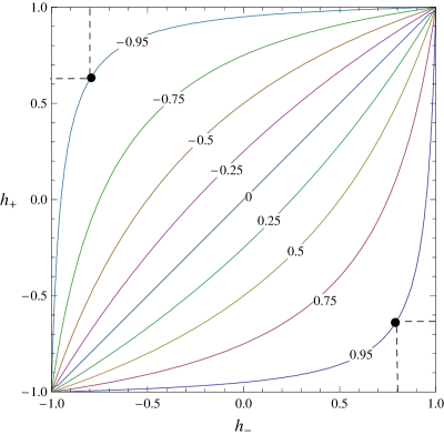
Figure 2: Contour plot in $(h_{+},h_{-})$–plane

4 Stability of polarization against variations of $P_{\rm eff}$

Extrapolations of $|\vec{P}|$ away from $P_{\rm eff}=\pm 1$ are more stable for $P_{\rm eff}=-1$ than for $P_{\rm eff}=+1$. Take, for example, the magnitude of the top quark polarization at threshold Eq. (5) and differentiate it w.r.t. $P_{\rm eff}$ at $P_{\rm eff}=\pm 1$. One finds

$$\frac{d|\vec{P}_{\rm thresh}\,|}{dP_{\rm eff}}=\pm\frac{1\pm A_{LR}}{1\mp A_{LR}}.$$ (10)

For $P_{\rm eff}=-1$ one has a slope of $-(1-A_{LR})/(1+A_{LR})=-0.42$ while one has a much larger positive slope of $(1+A_{LR})/(1-A_{LR})=+2.38$ for $P_{\rm eff}=+1$. This feature persists at higher energies [7].

Figure 3: Parametric plot of the orientation and the length of the polarization vector in dependence on the c.m. energy $\sqrt{s}$ for values $\theta=60^{\circ}$, $90^{\circ}$, $120^{\circ}$, and $150^{\circ}$ for $P_{\rm eff}=-1$ (solid lines) and $P_{\rm eff}=-0.95$ (dashed lines). The three tics on the trajectories stand for $\sqrt{s}=500\,GeV$, $1000\,GeV$, and $3000\,GeV$.

Figure 4: Same as Fig.4 but for $P_{\rm eff}=+1$ (solid lines) and $P_{\rm eff}=+0.95$ (dashed lines).

5 Longitudinal and transverse polarization
$P^{(\ell)}$ vs. $P^{(tr)}$ for general energies

In Figs. 4 and 4 we plot the longitudinal component $P^{(\ell)}$ and the transverse component $P^{(tr)}$ of the top quark polarization for different scattering angles $\theta$ and energies $\sqrt{s}$ starting from threshold up to the high energy limit. $P^{(tr)}$ is the transverse polarization component perpendicular to the momentum of the top quark in the scattering plane. Fig. 4 is drawn for $P_{\rm eff}=(-1,-0.95)$ and Fig. 4 for $P_{\rm eff}=(+1,+0.95)$. The apex of the polarization vector $\vec{P}$ follows a trajectory that starts at $\vec{P}=P_{\rm thresh}(-\cos\theta,\sin\theta)$ and $\vec{P}=P_{\rm thresh}(\cos\theta,-\sin\theta)$ for negative and positive values of $P_{\rm eff}$, respectively, and ends on the line $P^{(tr)}=0$. The two $60^{\circ}$ trajectories for $60^{\circ}$ show that large values of the size of the polarization $|\vec{P}|$ close to the maximal value of $1$ can be achieved in the forward region for both $P_{\rm eff}\sim\mp 1$ and at all energies. However, the two figures also show that the option $P_{\rm eff}\sim-1$ has to be preferred since the $P_{\rm eff}=-1$ polarization is more stable against variations of $P_{\rm eff}$ whereas the polarization in Fig. 4 has changed considerably when going from $P_{\rm eff}=1$ to $P_{\rm eff}=0.95$.

The plots Figs. 4 and 4 are drawn for NLO  QCD. At NLO there is also a normal component $P^{(n)}$ generated by the one–loop contribution which, however, is quite small (of $O(3\%))$.

6 Summary

The aim of the investigation in [7] was to maximize and to minimize the polarization vector of the top quark $\vec{P}=\vec{P}\,(P_{\rm eff},\sqrt{s},\cos\theta)$ by tuning the beam polarization. Let us summarize our findings.

A. Maximal polarization
Large values of $\vec{P}$ can be realized for $P_{\rm eff}\sim\pm 1$ at all intermediate energies. This is particularly true in the forward region where the rate is highest. Negative large values for $P_{\rm eff}$ with aligned beam helicities ($h_{-}h_{+}$ neg.) are preferred for two reasons. First there is a further gain in rate apart from the helicity alignment factor $(1-h_{-}h_{+})$ due to the fact that generally $\sigma_{LR}>\sigma_{RL}$ as explained after (8) . Second, the polarization is more stable against variations of $P_{\rm eff}$.

B. Minimal polarization
Close to zero values of the polarization vector $\vec{P}$ can be achieved for $P_{\rm eff}\sim 0.4$. Again the forward region is favoured. In order to maximize the rate for the small polarization choice take quadrant IV in the $(h_{-},\,h_{+})$–plane.

Acknowledgements: J.G.K. would like to thank X. Artru and E. Christova for discussions and G. Moortgat-Pick for encouragement. We thank B. Melić and S. Prelovsek for their participation in this project. The work of S. G. is supported by the Estonian target financed project No. 0180056s09, by the Estonian Science Foundation under grant No. 8769 and by the Deutsche Forschungsgemeinschaft (DFG) under grant 436 EST 17/1/06.

References

- [1] E. Christova and D. Draganov, Phys. Lett. B 434 (1998) 373
-
[2]
M. Fischer, S. Groote, J. G. Körner, M. C. Mauser and B. Lampe,
Phys. Lett. B 451 (1999) 406 - [3] M. Fischer, S. Groote, J. G. Körner and M. C. Mauser, Phys. Rev. D 65 (2002) 054036
- [4] S. Groote, W. S. Huo, A. Kadeer and J. G. Körner, Phys. Rev. D 76 (2007) 014012
- [5] J. A. Aguilar-Saavedra and J. Bernabeu, Nucl. Phys. B 840 (2010) 349
- [6] J. Drobnak, S. Fajfer and J. F. Kamenik, Phys. Rev. D 82 (2010) 114008
- [7] S. Groote, J. G. Körner, B. Melić and S. Prelovsek, Phys. Rev. D 83 (2011) 054018
-
[8]
X. Artru, M. Elchikh, J. -M. Richard, J. Soffer and O. V. Teryaev,
Phys. Rept. 470 (2009) 1 - [9] G. Alexander, J. Barley, Y. Batygin, S. Berridge, V. Bharadwaj, G. Bower, W. Bugg and F. J. Decker et al., Nucl. Instrum. Meth. A 610 (2009) 451