Magnetic anisotropy of elongated thin ferromagnetic nano-islands for artificial spin ice arrays

Abstract

The energetics of thin elongated ferromagnetic nano-islands is considered for some different shapes, aspect ratios, and applied magnetic field directions. These nano-island particles are important for artificial spin-ice materials. For low temperature, the magnetic internal energy of an individual particle is evaluated numerically as a function of the direction of a particle’s net magnetization. This leads to estimations of effective anisotropy constants for (1) the easy axis along the particle’s long direction, and (2) the hard axis along the particle’s thin direction. A spin relaxation algorithm together with fast Fourier transform for the demagnetization field is used to solve the micromagnetics problem for a thin system. The magnetic hysteresis is also found. The results indicate some possibilities for controlling the equilibrium and dynamics in spin-ice materials by using different island geometries.

I Introduction: Elongated thin ferromagnetic nano-islands

Disordered and frustrated magnetic states such as those present in artificial spin ices Wang06 ; Remhof08 continue to draw interest, due to their competing ground states, magnetic monopole excitations Castel08 , string excitations Mol09 ; Mol10 ; Morgan11 ; Moller09 and the difficulty to achieve thermal equilibrium. Those systems are composed from elongated magnetic islands or particles of some length $L_{x}$ (several hundred nanometers) and width $L_{y}$ grown or etched lithographically to a small height $L_{z}$ on a substrate, whose geometric demagnetization effects (effectively, internal dipolar interactions) lead to a strong magnetic anisotropy. The typical islands have $L_{z}$ much less than $L_{x}$ or $L_{y}$. Obviously any very thin magnet acquires an effective easy-plane anisotropy Gioia97 , and if the particle is narrow as well, the long direction becomes an easy axis. The demagnetization field within an individual particle is responsible for this, making the plane of the island ($xy$-plane) an easy plane, and the $x$-axis an easy axis. Then net magnetic moment $\vec{\mu}$ acts somewhat like an Ising variable with a defined easy axis $\hat{x}$. These islands are arranged into ordered arrays to produce, for example, square lattice or kagome lattice artificial spin-ices. The analysis of spin ice models assumes that such particles have only the two states with $\vec{\mu}$ either aligned or anti-aligned to the particle’s easy axis. The dipolar interaction between different particles on one of the spin-ice lattices leads to the ice-rules, such as the “two in / two out” rule for the square lattice and pyrochlore spin ices Castel08 . Such ice rules are only energetic preferences, however, and only indicate the preferred states of the magnetic moments. They are not absolute rigid statements about the allowed states. Thus, the intention here is to investigate the energetics of the fluctuations away from this Ising aligned state, in the individual elliptical islands that are used to compose a spin-ice system.

At some level, there must be transitions between these Ising-like states. An individual particle may contain thousands of atomic spins, leading to a substantial energy barrier that must be surpassed to flip the Ising state of a particle. Hence, the dynamics is greatly constrained by such energy barriers. It is our interest here to discuss how this barrier depends on the particular geometry of the islands, and make some evaluations of the dependence of the effective potential on the island shape and height. The types of shapes we consider are ellipses. Thin single domain ellipses were studied by Wei et al. Wei03 , who found that the reversal process involves close to a uniform Stoner-Wohlfarth rotation, but with reduced energy barriers due to some non-uniformity of the magnetization. However, we find here that for high-aspect ratio ellipses, this non-uniformity is minimal and a uniform rotation model could be very useful.

Although the theory for spin ice has been developed for Ising-like magnetic moments, their dynamics requires a different model. In reality, the underlying magnetic moment must be evolving from much more complex dynamics. The reversal of an individual island, in the dipolar fields of its surrounding islands, must be a complex process, and could involve the motion of domain walls and vortices within the individual particles, or an impeded rotation of the local magnetization mostly in unison. But in the assumption of strong ferromagnetic exchange inside a particular particle, and a uniform externally applied field, one can investigate the reversal process using different approaches to the micromagnetics Suess06 , and see whether vortices or domain walls play any significant role. Especially, one can investigate whether there are intermediate metastable vortex or domain-wall states as steps of the reversal. To a great extent for the thin elliptical particles considered here, the reversal proceeds mostly as a nearly uniform but impeded rotation of the magnetization of the particle Wei03 , although the switching fields are reduced compared to a perfectly uniform rotation. Hence, the idea of an Ising spin for a particle can be replaced by a three-dimensional magnetic moment $\vec{\mu}$, moving in some anisotropy potential, but free to point in any direction, if enough energy becomes available to it.

Obviously, by changing the aspect ratios $g_{1}\equiv L_{x}/L_{y}$ and $g_{3}\equiv L_{x}/L_{z}$ of the particle, its effective anisotropy changes. The deviation of the ratio $L_{x}/L_{y}$ from $1$ determines the strength of an easy-axis anisotropy constant, call it $K_{1}$, for the net magnetic moment to rotate within the $xy$ plane. The other aspect ratio of length to thickness, $L_{x}/L_{z}$, determines the difficulty for the magnetic moment $\vec{\mu}$ to tilt out of the $xy$ plane. Thus it determines the strength of a hard axis anisotropy constant, call it $K_{3}$. The goal here is to make some accurate estimates for these constants, and in the process, to justify a more generalized description of the magnetic dynamics, not based on an Ising variable, but rather, on an effective three-dimensional magnetic moment, that is allowed to make deviations from the Ising axis. For a particle whose hard axis is along $\hat{z}$ and easy axis is along $\hat{x}$, an effective potential that approximately represents their energies is shown to be

$$E=E_{0}+K_{1}\left[1-(\hat{\mu}\cdot\hat{x})^{2}\right]+K_{3}(\hat{\mu}\cdot\hat{z})^{2}$$ (1)

where $\hat{\mu}$ is the unit vector pointing in the direction of the particle’s net magnetic moment. $E_{0}$ is the energy when the magnetic moment $\hat{\mu}$ is along the easy axis. This type of potential is continuous, in contrast to the two-state Ising particle, having a well-defined energy barrier, and having a more realistic dynamics. Further, it will give the possibility of controlling the thermodynamics of spin-ices via changes or variations in the nano-island structure, that can modify the energy barrier.

The calculational approach is a modification of usual micromagnetics Cervera99 ; Garcia03 , as follows. A particle is partitioned into cells of size $a\times a\times L_{z}$, under the assumption of the local magnetization $\vec{M}(\vec{r})$ being independent of the $z$-coordinate (along the thin dimension). Thus, there is only a single layer of cells in the $xy$-plane, with the desired shape, say, an ellipse of major diameter $L_{x}$ and minor diameter $L_{y}<L_{x}$. The saturated magnetization in each cell interacts with the neighboring cells by ferromagnetic exchange, an externally applied magnetic field, and interacts with all cells via the demagnetization field. The demagnetization field is calculated using an effective Green’s function that applies for thin systems Huang03 , see below, with the calculation accelerated by using a 2D fast Fourier transform (FFT). To evolve towards the nearest (possibly meta-) stable magnetic state, we do not use integration of the Landau-Gilbert spin dynamics equations with damping. Instead, a faster procedure is to use a local spin-alignment algorithm, that involves no damping parameter. In one step of this algorithm, each cell’s magnetic moment is pointed towards the local total magnetic field that is instantaneously producing a torque on that cell. The same procedure is applied to all cells, then, the demagnetization fields are recalculated, and the process is repeated iteratively until a desired tolerance is reached. A microscopic uniaxial anisotropy energy is also included, although using a strength that would be typical for Permalloy, it is almost irrelevant when compared to the exchange and demagnetization effects. We have checked that this procedure gives the same final states as integration of the Landau-Gilbert equations with damping.

The internal magnetic energy $E_{\rm int}$ of the particle is calculated. This is the total magnetic energy minus the interaction energy with the applied magnetic field, $-\vec{\mu}\cdot\vec{H}_{\rm ext}$. An applied magnetic field is used in the calculations to move the net magnetic moment around, while it as well maps out the hysteresis loop. In one set of simulations, the hysteresis loop was calculated with the applied field axis within the $xy$-plane at some angle $\phi_{H}$ to the $x$-axis. There, the magnetization makes an angle $\phi_{m}$ to the $x$-axis. Then the internal energy could be found as a function $E_{\rm int}(\phi_{m})$, from which the anisotropy constant $K_{1}$ is determined, by fitting to (1) in the form,

$$E_{\rm int}(\phi_{m})=E_{0}+K_{1}\sin^{2}\phi_{m}.$$ (2)

In another set of simulations, the applied field was set in the $xz$-plane, at some angle $\theta_{H}$ to the $x$-axis. This tilts the net magnetic moment towards the $z$-axis by an angle $\theta_{m}$ from the $x$-axis. Thus it gives $E_{\rm int}(\theta_{m})$, which depends on both constants $K_{1}$ and $K_{3}$, according to

$$E_{\rm int}(\theta_{m})=E_{0}+(K_{1}+K_{3})\sin^{2}\theta_{m}.$$ (3)

This allows anisotropy constant $K_{3}$ to be determined from the net stiffness, $K_{13}\equiv K_{1}+K_{3}$. It is important to note, that these potential functions $E_{\rm int}(\phi_{m})$ and $E_{\rm int}(\theta_{m})$ found this way do not depend on the particular angle chosen between the applied field and the $x$-axis.

In the following sections the Hamiltonian and algorithm is further specified. Some details about the demagnetization field calculation are given, especially concerning the Greens function. Finally the results for elliptic particles are discussed.

II The particle model and its energetics

We consider thin elliptical particles with dimensions $L_{x}\times L_{y}\times L_{z}$, where $L_{x}$ and $L_{y}$ refer to the major and minor diameters for the elliptical particles. The approach for a thin system has been presented in Ref. Wysin2010 ; some of the main points towards finding the spatial structure of magnetization $\vec{M}(\vec{r})$ and the particle’s internal energy are summarized here.

The system is partitioned into cells of size $a\times a\times L_{z}$ on a square lattice grid, where there is saturation magnetization $M_{s}$ within each cell. Thus a selected cell $i$ has a magnetic moment ${\bf m}_{i}=M_{s}a^{2}L_{z}\hat{m}_{i}$, that points in the direction of the unit vector $\hat{m}_{i}$ and has magnitude $\mu_{\rm cell}=M_{s}a^{2}L_{z}$. There is only a single layer of cells used, under the assumption that the perpendicular demagnetization effect leads to magnetization nearly independent of $z$, for the thin systems under consideration.

The exchange interaction in continuum theory is taken in terms of the exchange stiffness $A$ (about 13 pJ/m for Py) as a volume integral,

$${\cal H}_{\rm ex}=A\int dV~{}\nabla\hat{m}\cdot\nabla\hat{m}.$$ (4)

where $\hat{m}=\vec{M}/M_{s}$ is the local reduced magnetization. When expanded on the square lattice of cells, this is equivalent to a nearest neighbor exchange term for the cells,

$${\cal H}_{\rm ex}=-J\sum_{(i,j)}\hat{m}_{i}\cdot\hat{m}_{j},\hskip 14.45377ptJ=2AL_{z}.$$ (5)

A uniaxial anisotropy energy $K$ (about 100 J/m³ for Py) is included as another volume integral

$${\cal H}_{\rm uni}=-K\int dV~{}(\hat{m}\cdot\hat{u})^{2}\rightarrow-Ka^{2}L_{z}\sum_{i}\,(\hat{m}_{i}\cdot\hat{u})^{2},$$ (6)

where the anisotropy axis here is taken as $\hat{u}=\hat{x}$. The externally applied magnetic field involves an energy of $-\vec{B}\cdot\vec{\mu}$ for any dipole, so

$${\cal H}_{\rm B}=-\int dV~{}\mu_{0}\vec{H}_{\rm ext}\cdot\vec{M}\rightarrow-\mu_{0}M_{s}a^{2}L_{z}\sum_{i}\,\vec{H}_{\rm ext}\cdot\hat{m}_{i}.$$ (7)

Finally, the most important part of the interactions is the demagnetization field or dipolar interaction. Once the cells are defined on the grid with lattice spacing $a$, their dipole interaction could be described by a Hamiltonian,

$${\cal H}_{\rm dd}=-\frac{\mu_{0}}{4\pi}\mu_{\rm cell}^{2}\sum_{i>j}\frac{\left[3(\hat{m}_{i}\cdot\hat{r}_{ij})(\hat{m}_{j}\cdot\hat{r}_{ij})-\hat{m}_{i}\cdot\hat{m}_{j}\right]}{\left|\vec{r}_{i}-\vec{r}_{j}\right|^{3}}$$ (8)

However, this does not take into account the fact that the system is very thin. The demagnetization field can be found very accurately for thin systems using a Greens function approach Huang03 . To do that, instead we start from the continuum dipolar energy,

$${\cal H}_{\rm dd}=-\frac{1}{2}\mu_{0}\int~{}dV~{}\vec{H}_{M}\cdot\vec{M}$$ (9)

where $\vec{H}_{M}=-\vec{\nabla}\Phi_{M}$ is the demagnetization field at some point, and $\Phi_{M}$ is its corresponding scalar magnetic potential. That field is produced by all the dipoles, according to a Poisson equation for magneto-statics:

$$-\nabla^{2}\Phi_{M}=\rho_{M},\quad{\rm where}\quad\rho_{M}=-\vec{\nabla}\cdot\vec{M}.$$ (10)

Further, the discontinuity at the surfaces of the particle can be modeled as a magnetic surface charge density, $\sigma_{M}=\vec{M}\cdot\hat{n}$, where $\hat{n}$ is the outward normal. In particular, that gives charge densities of opposite signs, $\sigma_{M}=\pm M_{z}$ on the upper and lower faces at $z=0,L_{z}$, respectively, under the assumption of uniform magnetization not depending on $z$ within the cells. The field of those surface charges is responsible for keeping the magnetization close to the $xy$ plane. There are also surface magnetic charges at the edges of the island but those can be included into a localized volume charge for the cells there. But whether the magnetic charges are surface charges or volume charges makes no physical difference, however, and the solution of the Poisson equation is formally

$$\Phi(\vec{r}\,)=\int d^{3}r^{\prime}~{}\frac{\rho(\vec{r}\,^{\prime})}{4\pi\left|\vec{r}-\vec{r}\,^{\prime}\right|}$$ (11)

This can be used to find the demagnetization field at the point $\vec{r}=(x,y,z)$, and then averaging that result over $z$ from $z=0$ to $z=L_{z}$. The resulting demagnetization field at a cell centered at $(x,y)$ has a vertical component $H_{M,z}$ and some in-plane component $\vec{H}_{M,xy}$. These are given by convolutions with appropriate 2D Green’s functions, involving only the in-plane position, denoted here as $\tilde{r}=(x,y)$. For the vertical demagnetization component, one gets

$${H}_{M,z}(\tilde{r})=\int d^{2}\tilde{r}\,^{\prime}~{}G_{z}(\tilde{r}-\tilde{r}\,^{\prime})~{}M_{z}(\tilde{r}\,^{\prime}),\quad\tilde{r}\equiv(x,y)$$ (12)

$$G_{z}(\tilde{r})=\frac{1}{2\pi L_{z}}\left[\frac{1}{\sqrt{\tilde{r}^{2}+L_{z}^{2}}}-\frac{1}{\left|\tilde{r}\right|}\right],\quad\tilde{r}^{2}\equiv x^{2}+y^{2}$$ (13)

For the in-plane components, there is

$$\vec{H}_{M,xy}(\tilde{r})=\int d^{2}\tilde{r}\,^{\prime}~{}\vec{G}_{xy}(\tilde{r}-\tilde{r}\,^{\prime})~{}{\rho}(\tilde{r}\,^{\prime}).$$ (14)

$$\vec{G}_{xy}(\tilde{r})=\frac{\hat{e}_{\tilde{r}}}{2\pi L_{z}}\left[\sqrt{1+\left(\frac{L_{z}}{|\tilde{r}|}\right)^{2}}-1\right].$$ (15)

When applied, the unit vector $\hat{e}_{\tilde{r}-\tilde{r}\,^{\prime}}$ points from source point $\tilde{r}\,^{\prime}$ towards observation point $\tilde{r}$. There is a singularity in $G_{z}(\tilde{r})$ as $\tilde{r}\rightarrow 0$, which is handled by averaging $G_{z}$ over a region with the same area as the cells being used, see Ref.  Wysin2010 for further details on this averaging of the Green’s functions.

Together with appropriate finite-difference approximations for the magnetic charge density, these expressions are used to get the demagnetization field. The actual evaluation of these convolution integrals was performed as multiplication in reciprocal space using a 2D fast Fourier transform approach Sasaki97 . To simulate a free particle without the periodicity effects of the FFT (i.e., to avoid the wrap-around problem), the grid of the FFT is padded to a net size of $N_{x}\times N_{y}$, where $N_{x}$ and $N_{y}$ are the smallest powers of two satisfying $N_{x}\geq 2L_{x}/a$ and $N_{y}\geq 2L_{x}/a$. Because we consider elongated particles, the calculations can be very fast due to $N_{y}$ being rather small compared to $N_{x}$, for high aspect ratio particles. The FFT approach ends up giving the demagnetization field at the cell center positions (as well as at other points outside the particle, due to the padding).

It is convenient to measure magnetic fields $\vec{H}_{\rm ext}$ and $\vec{H}_{M}$ in units of the saturation magnetization $M_{s}$, just as done for the magnetization, $\hat{m}=\vec{M}/M_{s}$, and define the dimensionless fields,

$$\vec{h}_{\rm ext}\equiv\frac{\vec{H}_{\rm ext}}{M_{s}},\hskip 21.68121pt\vec{h}_{M}\equiv\frac{\vec{H}_{M}}{M_{s}}.$$ (16)

The basic (and largest) unit of energy is the exchange $J$ between neighboring cells. Then the total effective Hamiltonian can be written in units of $J$ as

$${\cal H} + -J\left\{\sum_{(i,j)}\hat{m}_{i}\cdot\hat{m}_{j}\right.$$

$$+ \left.\left(\frac{a}{\lambda_{\rm ex}}\right)^{2}\sum_{i}\left[\kappa(\hat{m}_{i}\cdot\hat{u})^{2}+\left(\frac{1}{2}\vec{h}_{M,i}+\vec{h}_{\rm ext}\right)\cdot\hat{m}_{i}\right]\right\}.$$

This is written in terms of the ferromagnetic exchange length $\lambda_{\rm ex}$ and the scaled dimensionless uniaxial anisotropy $\kappa$, defined as

$$\lambda_{\rm ex}=\sqrt{\frac{2A}{\mu_{0}M_{S}^{2}}},\quad\quad\kappa=\frac{K}{\mu_{0}\,M_{s}^{2}}.$$ (18)

The magnetic internal energy $E_{\rm int}$ is of most interest. That is this Hamiltonian, but with the interaction with the external magnetic field (the last term) removed.

For the calculations we used the values for Permalloy, $M_{s}\approx 860$ kA/m, $A\approx$ 13 pJ/m, $K\approx 100$ J/m³, then these give $\lambda_{\rm ex}\approx 5.3$ nm and $\kappa\approx 1.1\times 10^{-4}$. Due to this small value of $\kappa$, in most of the calculations the intrinsic uniaxial anisotropy energy is negligible compared to the other energies of the system. In most of the simulations the cell size was $a=2.0$ nm, except for the smallest high aspect ratio particles, where values as low as $a=0.5$ nm were used, to produce a smoother edge to the particle. These are sufficiently less than the exchange length to give a reliable description of the internal magnetic structure.

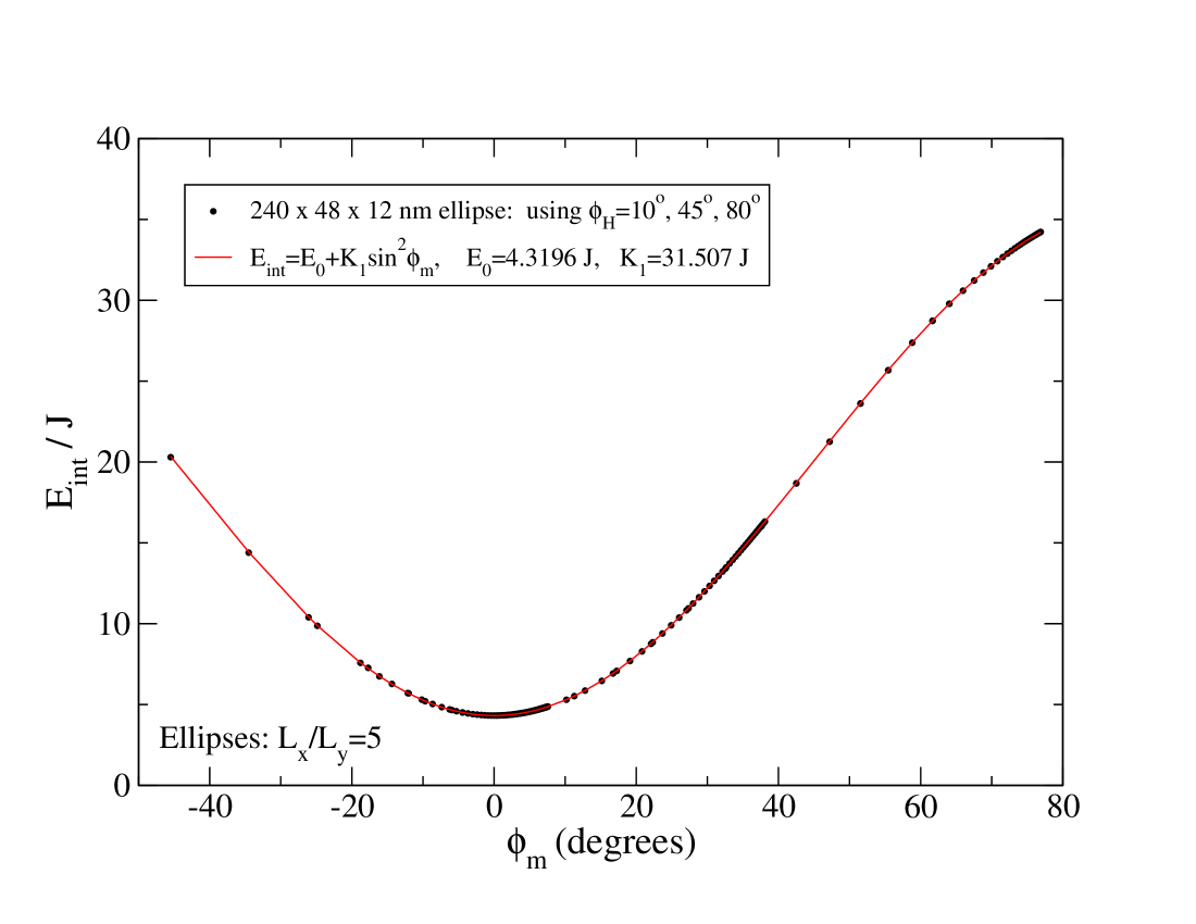
Figure 1: (Color online) The in-plane potential of an elliptical particle with a 5:1 aspect ratio, mapped out while determining the hysteresis loop (Fig. 3). The angle $\phi_{m}$ is the direction of the net particle moment $\vec{\mu}$ in the easy-plane. The points come from simulations at the different indicated angles $\phi_{H}$ of the applied field from the long axis; all fall onto the same curve. The fit gives a reliable estimate of anisotropy constant $K_{1}$.

III Calculation procedures

The iteration procedure that moves the system towards the nearest local equilibrium is a local spin relaxation algorithm Wysin96 , that points each cell’s magnetic moment $\vec{m}_{i}$ (or its unit vector $\hat{m}_{i}$) along its local magnetic field $\vec{B}_{i}$. That local field enters the undamped dynamic equation of motion,

$$\frac{d\vec{m}_{i}}{dt}=\gamma\vec{m}_{i}\times\vec{B}_{i},$$ (19)

and it is given by the variation of the Hamiltonian,

$$\vec{B}_{i} = -\frac{\delta{\cal H}}{\delta\vec{m}_{i}}=-\frac{1}{\mu_{\rm cell}}\frac{\delta{\cal H}}{\delta\hat{m}_{i}}=\frac{J}{\mu_{\rm cell}}\left\{\sum_{\rm nbrs}\hat{m}_{j}\right.$$

$$+ \left.\left(\frac{a}{\lambda_{\rm ex}}\right)^{2}\left[2\kappa(\hat{m}_{i}\cdot\hat{u})\hat{u}+\frac{1}{2}\vec{h}_{M,i}+\vec{h}_{\rm ext}\right]\right\}$$

Alternatively, this is the same as

$$\vec{B}_{i} = \mu_{0}M_{s}\left\{\left(\frac{\lambda_{\rm ex}}{a}\right)^{2}\sum_{\rm nbrs}\hat{m}_{j}\right.$$

$$+ \left.\left[2\kappa(\hat{m}_{i}\cdot\hat{u})\hat{u}+\frac{1}{2}\vec{h}_{M,i}+\vec{h}_{\rm ext}\right]\right\}$$

Either way, these define a unit vector along which to point the magnetic moment of cell $i$, $\hat{m}_{i}\rightarrow\hat{m}_{i}^{\prime}$, where

$$\hat{m}_{i}^{\prime}=\hat{b}_{i}=\frac{\vec{B}_{i}}{|\vec{B}_{i}|}.$$ (22)

The alignment of $\hat{m}_{i}$ parallel to $\hat{b}_{i}$ is performed for every site of the grid, after which the demagnetization field must be recalculated. The process moves the system towards lower energy. Each cell would stop moving if all became simultaneously aligned self-consistently with their local magnetic fields. This does not insure a global energy minimum, however, and the procedure does have the capability to generate the hysteresis loops. The iteration is started from a partially aligned state of the cell dipoles, which are given some small random fluctuations away from perfect alignment. For the hysteresis calculation, though, the last relaxed state at one applied field is the initial state for the next value of applied field.

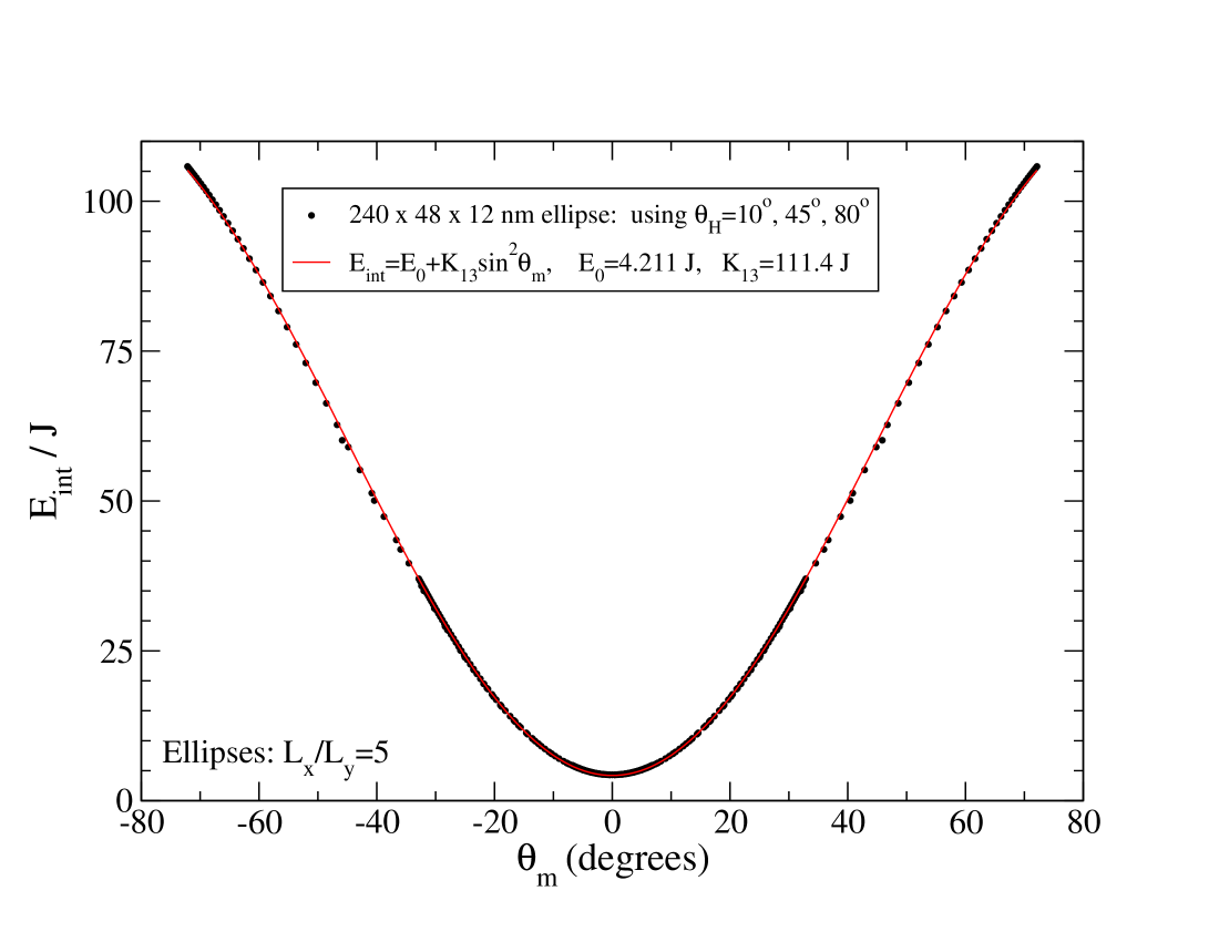
Figure 2: (Color online) The out-of-plane potential of the same elliptical particle with a 5:1 aspect ratio as in Fig. 1, mapped out while determining the hysteresis loop (Fig. 4). The angle $\theta_{m}$ is the tilting of the net particle moment $\vec{\mu}$ out of the easy-plane. The points from simulations at different angles $\theta_{H}$ of the applied field are combined into one curve. The fit gives a reliable estimate of the combined anisotropy constant $K_{13}=K_{1}+K_{3}$.

As the iteration proceeds, periodically (every 200 iterations of the system) the total magnetic moment $\vec{\mu}$ of the particle is calculated, by summing over the cell dipoles,

$$\vec{\mu}=(\mu_{x},\mu_{y},\mu_{z})=\mu_{\rm cell}\sum_{i}\hat{m}_{i}$$ (23)

The iteration is stopped when the changes in any component of $\vec{\mu}$ are less than 1 part in $5\times 10^{7}$ for two states separated by 200 iterations. This is actually a more stringent stopping requirement than waiting for the energy to converge to the same precision.

In one set of simulations, the applied magnetic field was directed within the $xy$-plane at an angle $\phi_{H}$ to the $x$-axis [$\vec{H}_{\rm ext}=H_{\rm ext}(\cos\phi_{H},\sin\phi_{H},0)$]. This results in the net magnetic moment $\vec{\mu}$ lying within the $xy$-plane, due to the strong perpendicular demagnetization. The moment makes some angle $\phi_{m}<\phi_{H}$ to the $x$-axis, calculated from $\phi_{m}=\tan^{-1}(\mu_{y}/\mu_{x})$. Thus, the in-plane potential energy function $E_{\rm int}(\phi_{m})$ could be found, by scanning in applied magnetic field strength along the chosen axis, and thereby calculating the hysteresis loop. Then $K_{1}$ was found by fitting to the form in (2).

In the other set of simulations, the magnetic field was applied tilting out of the $xy$-plane, making an angle $\theta_{H}$ to the $x$-axis, that is, $\vec{H}_{\rm ext}=H_{\rm ext}(\cos\theta_{H},0,\sin\theta_{H})$. This pulls $\vec{\mu}$ up an angle $\theta_{m}<\theta_{H}$ from the easy ($xy$) plane, where $\theta_{m}=\tan^{-1}(\mu_{z}/\mu_{x})$, and gives the opportunity to measure the potential $E_{\rm int}(\theta_{m})$. Again, the internal energy is calculated from the total Hamiltonian minus the interaction term with the applied external field. That energy was fitted to the out-of-plane potential (3), whose stiffness is due to the combination, $K_{13}=K_{1}+K_{3}$. Further, the potentials obtained did not depend on the choice of $\phi_{H}$ or $\theta_{H}$. This could be seen by combining the internal energy curves for applied field at 45^∘ and 80^∘ to the $x$-axis.

For the hysteresis curves, the total magnetic moment $\vec{\mu}$ was calculated, and normalized by the particle volume $V$ to get the averaged magnetization inside the particle, $\langle\vec{M}\rangle=\frac{\vec{\mu}}{V}$. Then the component of $\langle\vec{M}\rangle$ along the applied field axis is found,

$$\langle M_{h}\rangle\equiv\langle\vec{M}\rangle\cdot\hat{h}_{\rm ext}$$ (24)

After scaling by the saturation magnetization, this is plotted versus the applied field magnitude also scaled by saturation magnetization ($h_{\rm ext}=H_{\rm ext}/M_{s})$.

IV Results for elliptical particles

We considered thin elliptical particles with thicknesses all 1/20^th of the length, i.e., $g_{3}=L_{x}/L_{z}=20$, and aspect ratios $g_{1}=L_{x}/L_{y}=3,5$, and $8$. The lengths ranged from 120 nm to 480 nm. Some typical results for the internal energy curves are shown in Fig. 1 for the in-plane potential and Fig. 2 for the out-of-plane potential of an elliptical particle with $g_{1}=5$, with major axis 240 nm, minor axis 48 nm and thickness 12 nm. The potentials for in-plane motion of $\vec{\mu}$ fit very well to the functional form,

$$E_{\rm int}(\phi_{m})=E_{0}+K_{1}\sin^{2}\phi_{m}.$$ (25)

The constant $E_{0}$ is an irrelevant ground state energy when the particle is magnetized along its long axis. This same form also applies to the potential $E_{\rm int}(\theta_{m})$, but with a coefficient $K_{13}=K_{1}+K_{3}$. The fits are best for smaller particles, where the cells stay strongly aligned with each other, and the reversal can be considered close to a uniform rotation process, for the most part. For the larger particles (length $>400$ nm) this global alignment is lesser and the fits are good but with considerably greater $\chi^{2}$. Even so, the internal magnetization structure of the relaxed states tends to be close to uniform.

	$L_{x}=120$ nm	$L_{x}=240$ nm	$L_{x}=480$ nm
$g_{1}=2$	$K_{1}=6.35J$	$27.3J$	$111J$
$g_{1}=3$	$7.32J$	$31.9J$	$134J$
$g_{1}=5$	$6.96J$	$31.5J$	$133J$
$g_{1}=8$	$7.39J$	$29.5J$	$118J$

Table 1: Values of the in-plane anisotropy constant $K_{1}$ in units of $J=2AL_{z}$ for the indicated particle sizes and aspect ratios $g_{1}=L_{x}/L_{y}$. All of the particles calculated have $g_{3}=L_{x}/L_{z}=20$.

	$L_{x}=120$ nm	$L_{x}=240$ nm	$L_{x}=480$ nm
$g_{1}=2$	$K_{13}=79.0J$	$314J$	$1250J$
$g_{1}=3$	$50.7J$	$201J$	$804J$
$g_{1}=5$	$28.1J$	$111J$	$444J$
$g_{1}=8$	$15.7J$	$62.6J$	$250J$

Table 2: Values of the combined anisotropy constant $K_{13}$ in units of $J=2AL_{z}$ for the indicated particle sizes and aspect ratios $g_{1}=L_{x}/L_{y}$. All of the particles calculated have $g_{3}=L_{x}/L_{z}=20$.

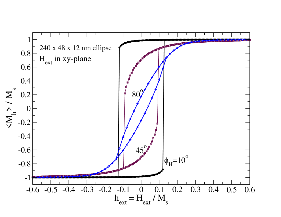
Figure 3: (Color online) Hysteresis loops for an elliptical particle as in Fig. 1 with an in-plane applied field at the indicated angles $\phi_{H}$ to the long axis of the particle.

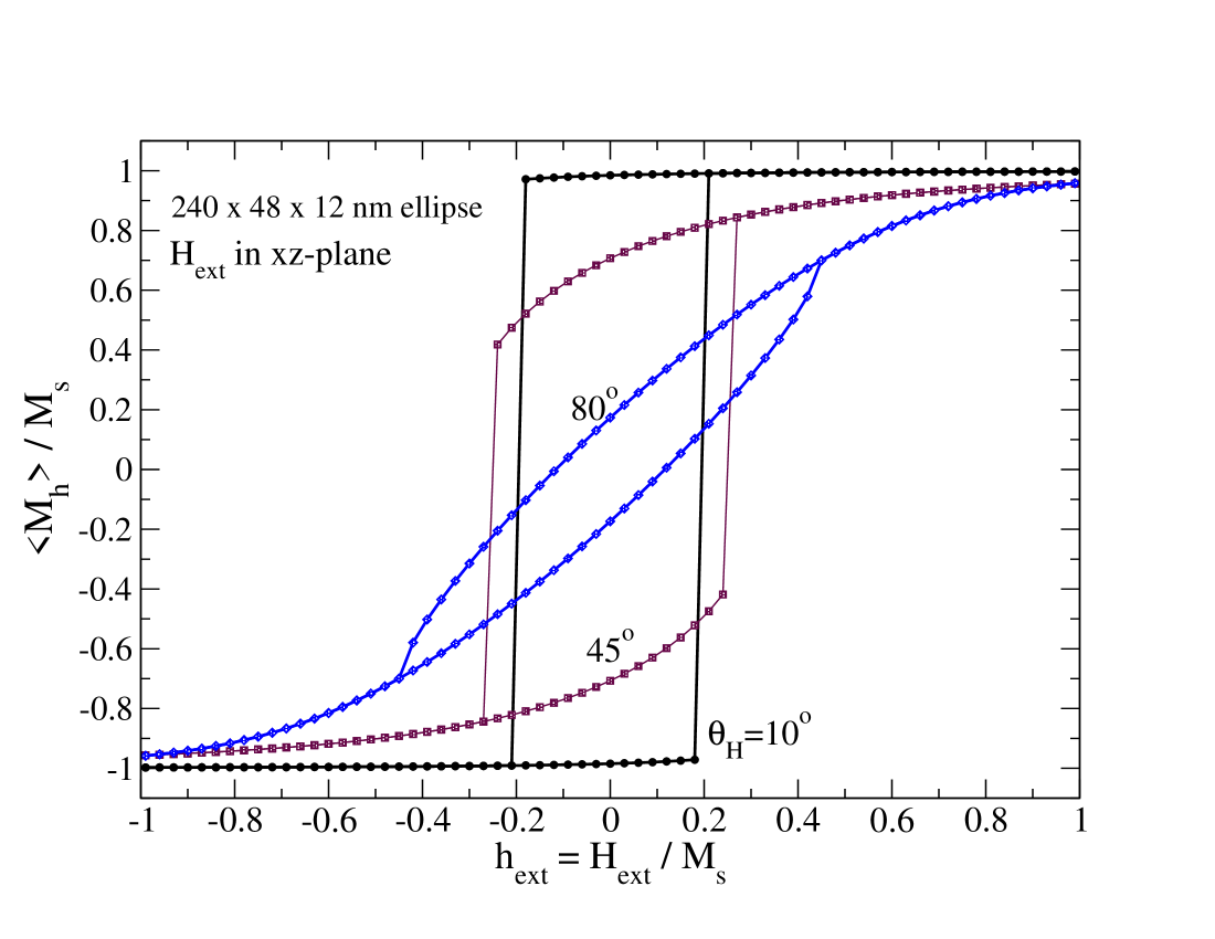
Figure 4: (Color online) Hysteresis loops for an elliptical particle as in Fig. 2 with the applied field tilted out of the $xy$-plane at the indicated angles $\theta_{H}$ from the long axis of the particle.

Fitting results are summarized in Tables 1 and 2, with the constants presented in units of $J=2AL_{z}$. The hard-axis anisotropy constant $K_{3}$ derived from those results is presented in Table 3. The constant $K_{3}$ is consistently stronger than the easy-axis constant $K_{1}$, as to be expected from the greater surface area of the lower and upper faces at $z=0,L_{z}$, compared to the very limited surface area of the edge of the ellipse. The energy unit $J$ itself varies according to the thickness. Thus it makes sense to also look at results for the constants in joules.

	$L_{x}=120$ nm	$L_{x}=240$ nm	$L_{x}=480$ nm
$g_{1}=2$	$K_{3}=72.7J$	$287J$	$1140J$
$g_{1}=3$	$43.4J$	$169J$	$670J$
$g_{1}=5$	$21.1J$	$79.9J$	$311J$
$g_{1}=8$	$8.30J$	$33.1J$	$132J$

Table 3: Values of the hard-axis anisotropy constant $K_{3}$ in units of $J=2AL_{z}$ for the indicated particle sizes and aspect ratios $g_{1}=L_{x}/L_{y}$. All of the particles calculated have $g_{3}=L_{x}/L_{z}=20$.

Generally, $K_{3}/J$ increases proportional to the area of the ellipse, $\frac{1}{4}\pi L_{x}L_{y}$, multiplied by the thickness $l_{z}$, so that in fact $K_{3}$ (in joules) is linearly proportional to the volume of the particles. Also, one sees that $K_{3}$ decreases with increasing aspect ratio for particles of the same length; this is because the particle volume is decreasing. On the other hand, $K_{1}/J$ depends very weakly on the aspect ratio for the particle sizes tested. In addition, the calculations suggest that $K_{1}$ increases somewhat faster than the particle volume. The weak dependence of $K_{1}$ on the shape of the ellipse (at these larger values of $g_{1}$) is surprising.

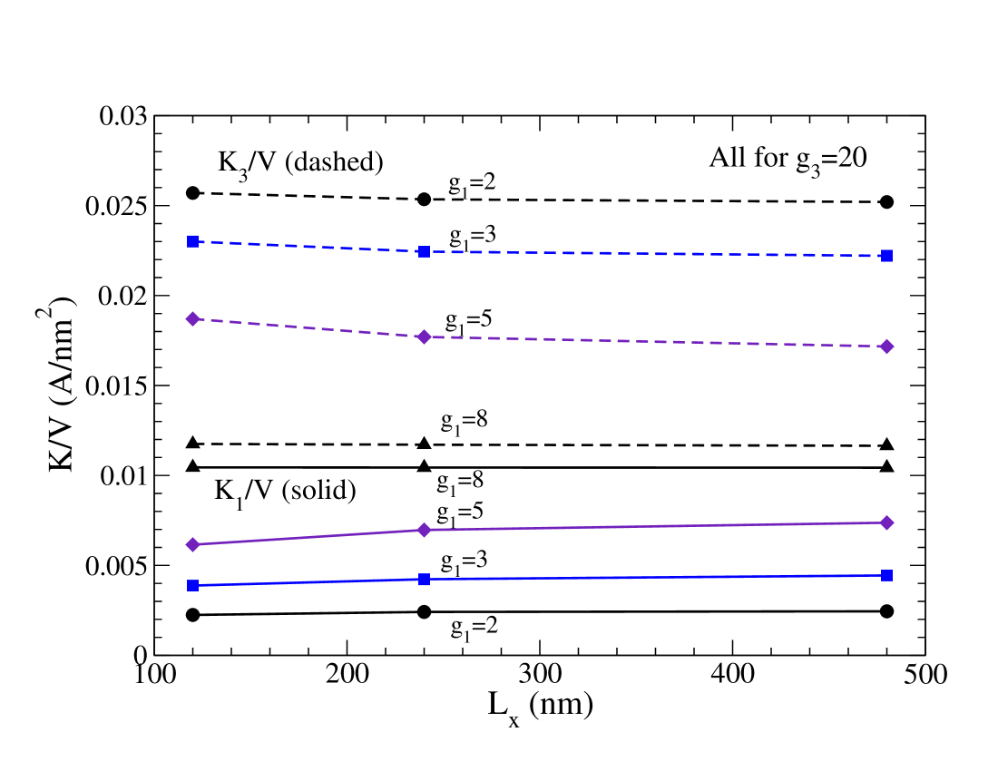
Figure 5: (Color online) The anisotropy constants $K_{1}$ (solid curves) and $K_{3}$ (dashed curves) scaled by elliptical particle volume, versus particle lengths, for the indicated $g_{1}$ aspect ratios. All data has $g_{3}=20$. The values of $K/V$ are given in units of $A$/nm², where $A$ is the exchange stiffness. $K_{1}/V$ increases with aspect ratio while $K_{3}/V$ decreases, and they become equal at high aspect ratio.

To clarify the results we also show the constants converted to energy densities, both $K_{1}/V$ and $K_{3}/V$ in joules/nm³, in Fig. 5. The actual units are the exchange stiffness $A$ (units of joules/nm) divided by squared nanometers. One finds very little dependence of either energy density constant, $K/V$, on the particle size, however, again it is clear that $K_{3}$ is always larger than $K_{1}$. Furthermore, the easy-axis anisotropy constant $K_{1}/V$ does increase rapidly with the in-plane aspect ratio $g_{1}$, and the relation could be close to a linear relationship. Although the values of $K_{3}/V$ are always greater than the corresponding $K_{1}/V$, these hard-axis energy densities $K_{3}/V$ decrease slightly with increasing aspect ratio $g_{1}$. At large aspect ratio, the two constants become nearly the same, which would have to be the case for a needle-shaped magnet.

IV.1 The magnetization structure

In the high aspect ratio particles, the magnetization states are very close to uniform, even when undergoing the reversal. The elongated particle has such a strong anisotropic effect that the magnetization cells move almost in a synchronized motion. For particles with smaller aspect ratio, one starts to see some weak variations in the magnetization inside the particle.

To get an idea of the size of this effect, some configurations are presented for ellipses with $g_{1}=2$, which has the strongest effect of all the particle shapes presented earlier. In Fig. 6 some configurations are shown for a $120\times 60\times 6$ nm particle, at different applied field strengths 45^∘ to the particle’s long ($+x$) axis. The points shown are at (a) close to saturation, (b) zero applied field, (c) a negative field close to reversal, and (d) a negative field just after reversal. For the most part, the magnetization stays nearly uniform for this relatively small particle.

Another example is presented in Fig. 7, like the first example, but $2\times$ larger in all three dimensions. The four configurations shown correspond to the same four types of states as presented for the smaller particle. The main difference here is that a nonuniform magnetic structure develops. At zero field, the structure points inward/outward towards the poles on the long axis. For the configurations just before and after reversal, a wave-like structure is present. These spatial variations are due to the dipolar interactions; in even lower aspect ratio particles ($g_{1}<2$), they lead to C-states and even vortices entering the particle.

Figure 6: Magnetic configurations for a $120\times 60\times 6$ nm particle with magnetic field applied at +45^∘ above a horizontal axis pointing to the right. The arrows are the coarse-grained averages of $3\times 3$ groups of cells. In (a), the external field is $h=0.20$; in (b) $h=0.0$; (c) $h=-0.030$, just before reversal; (d) $h=-0.032$, just after reversal.

Figure 7: Magnetic configurations for a $480\times 240\times 24$ nm particle with magnetic field applied at +45^∘ above a horizontal axis pointing to the right. The arrows are the coarse-grained averages of $9\times 9$ groups of cells. In (a), the external field is $h=0.20$; in (b) $h=0.0$; (c) $h=-0.025$, just before reversal; (d) $h=-0.027$, just after reversal. Note the enhanced curvature of the field compared to that in the smaller particle in Fig. 6.

IV.2 Particles with lower aspect ratio $g_{1}<2$

When $g_{1}\rightarrow 1$, the ellipse becomes circular and the easy-axis anisotropy must vanish. Using smaller $g_{1}$ is a way to produce particles with weaker easy-axis anisotropy constant. However, as the system becomes closer to circular, the lowest energy configuration, especially near zero applied magnetic field, tends to be nonuniform. The ground state can tend towards a C-state or a vortex state if the particle is of sufficient size. The above results do not apply to that situation, especially because the nonuniform magnetization cannot be mapped into the model of an individual magnetic moment moving in an effective potential.

To verify this, some particles were also calculated at small ellipticity, where $K_{1}\approx 0$, using $g_{1}=1.25$ and $g_{1}=1.11$. Generally, at these ratios, if there was a stable single-domain ground state (for smaller particles only), the tendency is for the moments to try to follow the border, and point inwards or outwards from the poles at the long ends. At larger particle size this tilting eventually moves the system irreversibly to a vortex ground state. Until the vortex state is reached, an effective potential can be estimated, however, from the practical point of view it may be of limited use.

IV.3 Thicker particles

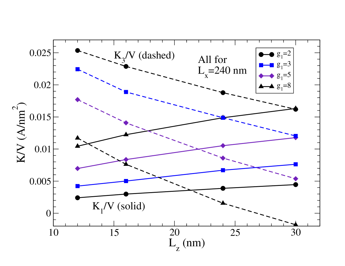
Figure 8: (Color online) The anisotropy constants $K_{1}$ (solid curves) and $K_{3}$ (dashed curves) scaled by elliptical particle volume, versus particle thicknesses, for the indicated $g_{1}$ aspect ratios. All the data is for particles of length $L_{x}=240$ nm. The $K_{3}/V$ constant crosses below zero for the thickest high-aspect-ratio particles, which have become needle-like and no longer satisfy the assumption of a thin particle. That is the case of a particle with only uniaxial anisotropy.

The particles with $g_{3}=20$ can be too thin to hold a magnetic moment stable against room-temperature thermal fluctuations. Thus it is important to consider the changes when thicker particles are used. Further calculations were carried out for 240 nm long particles to get results for $g_{3}=20,15,10,$ and $8$, corresponding to thicknesses of 12, 16, 24 and 30 nm, respectively. The results for $K_{1}/V$ and $K_{3}/V$ are shown in Fig. 8. As could be expected, the thicker particles have weaker out-of-plane anisotropy $K_{3}/V$, while $K_{1}/V$ increases due to the thicker lateral edges, but at a rate less than linear in the thickness. We expect that these per-volume energy constants have only very weak dependence on the particle length, as was already seen in the results presented above for 12.0 nm thickness.

V Conclusions and Discussion

The anisotropy properties of thin elliptical ferromagnetic particles have been estimated, based on a 2D micromagnetics model that employs Green’s functions for the calculation of the demagnetization fields. For the high-aspect-ratio particles being considered, the magnetization was found to be close to uniform inside the particles. Then it was possible to map out the changes in the internal energy versus the direction of the net magnetic moment $\vec{\mu}$, which itself acts as a collective coordinate. The typical particles tend to have stronger anisotropy in the hard-axis direction ($K_{3}/V$) than in the easy-axis direction ($K_{1}/V$), however, these two energy scales approach each other for needle-like particles, as expected. The results could be of practical application in the design and analysis of artificial spin-ice with desired dynamics, beyond the usual Ising energetics.

In the theoretical study of artificial spin ice materials, it is usual to replace the islands by point-like dipoles with an Ising-like behavior. Indeed, all theoretical calculations for the properties of these systems were obtained with this approach. However, a more realistic description of these artificial spin ices should require models beyond the Ising approximation, such as continuous magnetic moments with anisotropy considered in this work. In such a case, although the main properties of a spin ice system may not undergo strong alterations, several quantities would change their values. For instance, a recent work about the thermodynamics of the square lattice Silva+11 has suggested a possible phase transition in this system, occurring at a temperature of $7.2D$, where $D$ is the coupling constant of the dipolar interaction among the islands. Of course, the transition temperature or similar quantities should be dependent on the island sizes and anisotropies, but this dependence cannot be perceived with the Ising approach. It is very probable that the correct critical temperature must be much smaller than $7.2D$ since the total magnetic moment of an island has more degrees of freedom, and effectively moves in a softer potential. In addition, the properties must also be dependent on the islands’ shapes, etc. So, the results obtained here are of fundamental importance for developing this field not only theoretically but also experimentally, suggesting protocols for improving experiments, and including studies about their dynamics.

VI Acknowledgments

G.M. Wysin appreciates the hospitality of The Department of Physics at Universidade Federal de Viçosa where this work was carried out, and is grateful for the financial support of FAPEMIG grant BPV-00046-11 for visiting research professor while at UFV.

References

- (1) R.F. Wang, C. Nisoli, R.S. Freitas, J. Li, W. McConville, B.J. Cooley, M.S. Lund, N. Samarth, C. Leighton, V.H. Crespi and P. Schiffer, Nature 439, 303 (2006).
- (2) A. Remhof, A. Schumann, A. Westphalen, H. Zabel, N. Mikuszeit, E.Y. Vedmedenko, T. Last, and U. Kunze, Phys. Rev. B 77, 134409 (2008).
- (3) C. Castelnovo, R. Moessner and L. Sondhi, Nature 451, 42 (2008).
- (4) L.A.S. Mól, R.L. Silva, R.C. Silva, A.R. Pereira, W.A. Moura-Melo and B.V. Costa, J. Appl. Phys. 106, 03913 (2009).
- (5) L.A.S. Mól, W.A. Moura-Melo, and A.R. Pereira, Phys. Rev. B 82, 054434 (2010).
- (6) J.P. Morgan, A. Stein, S. Langridge, and C. Marrows, Nature Phys. 7, 75 (2011).
- (7) G. Möller and R. Moessner, Phys. Rev. B 80, 140409(R) (2009).
- (8) G. Gioia and R.D. James, Proc. R. Soc. London, Ser. A 453, 213 (1997).
- (9) Zung-Hang Wei, Mei-Feng Lai, Ching-Ray Chang, N.A. Usov, J.C. Wu and Jun-Yang Lai, J. Mag. Magn. Mater. 272-276, e563 (2004).
- (10) Dieter Suessa, Josef Fidlera and Thomas Schrefl, Handbook of Magn. Mater. 16 41 (2006).
- (11) Carlos J. García-Cervera, “Magnetic Domains and Magnetic Domain Walls,” Ph.D. thesis, New York University (1999).
- (12) Carlos J. García-Cervera, Zydrunas Gimbutas and Weinan E, J. Comp. Phys. 184, 37 (2003).
- (13) Zhongyi Huang, J. Comp. Math. 21, 33 (2003).
- (14) G.M. Wysin, J. Phys.: Condens. Matter 22, 376002 (2010).
- (15) J. Sasaki and F. Matsubara, J. Phys. Soc. Japan 66, 2138 (1997).
- (16) G.M. Wysin, Phys. Rev. B 54, 15156 (1996).
- (17) R.C. Silva, F.S. Nascimento, L.A.S. Mól, W.A. Moura-Melo and A.R. Pereira, arXiv: 1110.2427v1 (2011).