Magnetotransport in the Kondo model with ferromagnetic exchange interaction

Abstract

We consider the transport properties in an applied magnetic field of the spin $S=1/2$ Kondo model with ferromagnetic exchange coupling to electronic reservoirs, a description relevant for the strong coupling limit of underscreened spin $S=1$ Kondo impurities. Because the ferromagnetic Kondo interaction is marginally irrelevant, perturbative methods should prove accurate down to low energies. For the purpose of this study, we use a combination of Majorana diagrammatic theory with Density Matrix Numerical Renormalization Group simulations. In the standard case of antiferromagnetic Kondo exchange, we first show that our simple analytical technique recovers results for the $\mathcal{T}$-matrix and spin relaxation at weak coupling (above the Kondo temperature), that were previously obtained using functional renormalization tools. Considering then the ferromagnetic case, we demonstrate how the low-energy Kondo anomaly splits for arbitrary small values of the Zeeman energy, in contrast to fully screened Kondo impurities near the strong coupling Fermi liquid fixed point, and in agreement with recent experimental findings for spin $S=1$ molecular quantum dots.

I Introduction

Magnetotransport measurements in quantum dots allow to probe and tune the magnetic properties of nanostructures in a situation where the conductance is the only experimentally accessible quantity kastner_single-electron_1992 ; kastner_single_2000 . Cotunneling Zeeman spectroscopy under an applied voltage bias (i.e. in a process that does not electrically charge the quantum dot) can be used for instance to resolve the magnetic degeneracies of quantized energy levels, in similar spirit to usual optical analysis of atomic and molecular spectra [see Refs. roch_quantum_2008, ,Florens_Review, for an illustration in a two-electron quantum dot showing nearly degenerate singlet and triplet states]. A striking difference between quantum electronic transport and quantum optics is the easiness to realize the strong coupling of a discrete quantum system to a macroscopic number of external degrees of freedom, simply by contacting a single atom or molecule to metallic electrodes. While standard physical effects such as screening of the molecular charging energy Flensberg_screening and renormalizations of the atomic energy levels from quantum tunneling Holm ; Hauptmann ; Florens_Review can occur, these electronic setups opens a window to realize even more subtle many-body physics. One well-studied example is the Kondo effect in strongly tunnel-coupled quantum dots, where the magnetic screening of a spin active discrete level is performed by the bath of surrounding conduction electrons hewson_kondo_1997 ; goldhaber-gordon_kondo_1998 ; Cronenwett ; pustilnik_kondo_2004 ; GrobisReview . Interestingly, a variety of different and possibly exotic Kondo effects can occur in simple extensions of the Kondo model, several of which have been already realized experimentally [see Ref. Florens_Review, for a review]. While the standard Kondo effect involves a single spin $S=1/2$ coupled to a single electronic bath and leads to Fermi-liquid properties at low temperatures, a variant as simple as the spin $S=1$ case already presents anomalous transport properties roch_observation_2009 ; ParksUS . In the latter situation, conduction electrons cannot manage a full compensation of the magnetic impurity, resulting in a partially screened ground state with remanent $\log(2)$ entropy nozieres_kondo_1980 ; Mehta ; Koller ; Logan , yet unitary conductance at zero temperature $G=2e^{2}/h$ ($e$ is the electron charge and $h$ Planck’s constant). At low energy, the remanent magnetic degrees of freedom decouple from the electronic reservoirs (in a logarithmically slow fashion) and can be recovered by the application of an arbitrarily small Zeeman energy roch_observation_2009 . In contrast, the fully screened case of a spin $S=1/2$ leads to a singlet ground state with small but non-zero binding energy (the so-called Kondo temperature), which remains stable to the application of a magnetic fields that do not exceed the Kondo energy. These simple examples illustrate nicely how Zeeman spectroscopy can be used to distinguish between different types of many-body states roch_observation_2009 ; ParksUS .

The purpose of this paper is to investigate in detail the magnetotransport properties of such highly spin-polarizable underscreened $S=1$ Kondo impurities. We will make use here of the Nozières-Blandin description of the strong coupling fixed point in terms of the spin $S=1/2$ Kondo model with ferromagnetic Kondo exchange nozieres_kondo_1980 ; Mehta ; Koller . In that case, the magnetic interaction between the quantum impurity and the reservoirs can be treated by perturbative methods, allowing a controlled description of the transport properties. While one could use here the functional renormalization group methodologies previously developed to deal with the weak coupling regime of the antiferromagnetic case rosch_spectral_2003 ; rosch_kondo_2005 ; Schoeller ; Schuricht ; SchurichtAndergassen ; Kehrein , we will show that a comparable description can be achieved by more standard diagrammatic methods, thanks to an useful mapping of a single spin $S=1/2$ in terms of Majorana fermions parcollet_perturbative_2002 ; shnirman_spin-spin_2003 ; mao_spin_2003 ; bulaevskii_tunneling_2003 ; Florens_spinboson ; Mathias_Kondo_Thesis . The advantage of the Majorana technique with respect to more usual representations of the spin algebra lies in the recent understanding that spin dynamics can be described by one-particle Majorana Green’s functions, allowing the use of Dyson’s equation within the standard Feynman diagram expansion shnirman_spin-spin_2003 ; mao_spin_2003 ; Florens_spinboson . We will demonstrate that transport properties, as described by the $\mathcal{T}$-matrix of the Kondo problem, become similarly much simpler in the Majorana language. Indeed, while standard spin representations would require the computation of six-point correlation functions, the Majorana description expresses the $\mathcal{T}$-matrix as a four-point (two-body) fermionic correlator, where the RPA expansion for response functions can be used at leading logarithmic order. In order to test the method, we will first discuss how the usual weak-coupling description of the antiferromagnetic Kondo problem can be done within the Majorana diagrammatics, both at zero and finite magnetic field. A comparison to calculations based on the full density matrix extension hofstetter_generalized_2000 ; toth_density_2008 of the Numerical Renormalization Group (NRG) wilson_renormalization_1975 ; krishna-murthy_renormalization-group_1980 ; bulla_numerical_2008 , and previous analytical results rosch_spectral_2003 ; rosch_kondo_2005 will be made. We will then compute in detail the spin and transport dynamics of a ferromagnetically coupled quantum dot, both within the Majorana description and the NRG simulations, which are shown to match quantitatively, apart from a narrow domain near the Zeeman energy, where the NRG data lack sufficient energy resolution. Our main result concerns the Zeeman splitting of the $\mathcal{T}$-matrix in the ferromagnetic case, which we show to occur for arbitrarily small values of the applied magnetic field, in agreement with recent experimental findings for underscreened $S=1$ Kondo impurities in molecular quantum dots roch_observation_2009 . We also note that the ferromagnetic Kondo model considered here has also been recently proposed for some types of atomic size metallic constrictions on the basis of ab-initio calculations lucignano_kondo_2009 , but has received so far little attention Koller .

The paper is organized as follows. In Sec. II we introduce the Kondo model relevant for transport in quantum dots, discussing transport and magnetic properties. The differences between fully and partially screened moments, with the connection to the ferromagnetic Kondo problem, will be presented. In Sec. III, we develop the general Majorana diagrammatic method, both at zero and finite magnetic field. Results are finally given in Sec. IV, where both antiferromagnetically and ferromagnetically coupled spin $S=1/2$ impurities are considered, using the Majorana technique and NRG calculations. A critical discussion of numerical and analytical scheme is given in the conclusion.

II Kondo models for transport in quantum dots

II.1 Spin ${\bm{S}=1/2}$ case

The conductance $\mathcal{G}$ of a quantum dot is the main physical property that can be directly measured in quantum dot experiments. In semiconducting dots, electrons are confined to a small region with the help of top-gates, leading to a set of discrete energy levels subject to electron-electron interaction effects, and tunnel coupled to macroscopic reservoirs. Under a voltage bias, a finite current flows through the dot, and the conductance is determined by the transition rate of tunneling events from source to drain. The concept of single-electron transistor comes from the capacitive coupling in small confined dots, where the discrete number of electrons on the dot can be tuned using a backgate-voltage kastner_single-electron_1992 ; kastner_single_2000 . If the number of trapped electrons on the dot is odd, an electronic configuration with an unpaired spin obtains, leading usually to a $S=1/2$ state. The tunneling into the reservoirs then results in an effective antiferromagnetic exchange interaction $J>0$, which tends to suppress the magnetic state of the dot. The physical origin of the antiferromagnetic exchange is Pauli’s principle, which favors second order tunnel processes for antiparallel spin orientation of the electron in the dot and the ones in the reservoirs. This interaction can be described by the Kondo Hamiltonian:

$$H_{K}=J{\bf S}\;\cdot\!\!\sum_{\alpha_{1}\alpha_{2}}\sum_{{\bf k}_{1}{\bf k}_{2}}\sum_{\sigma_{1}\sigma_{2}}c^{\dagger}_{\alpha{\bm{k}}_{1}\sigma_{1}}\frac{\bm{\tau}^{\vphantom{\dagger}}_{\sigma_{1}\sigma_{2}}}{2}c^{\vphantom{\dagger}}_{\alpha{\bm{k}}_{2}\sigma_{2}}$$ (1)

where $\bm{\tau}$ denotes the vector $\bm{\tau}=\begin{pmatrix}\tau^{x},&\tau^{y},&\tau^{z}\end{pmatrix}$ formed by the three Pauli matrices. For simplicity we have assumed here symmetric coupling to the left and right reservoirs. Besides the quantized spin $\bm{S}$ in the dot, we have introduced fermion operators describing electrons in the reservoirs, as given by the Hamiltonian:

$$H_{0}=\sum_{{\bm{k}}\sigma\alpha}\epsilon^{\vphantom{\dagger}}_{\bm{k}}c^{\dagger}_{\alpha{\bm{k}}\sigma}c^{\vphantom{\dagger}}_{\alpha{\bm{k}}\sigma},$$ (2)

where the operator $c^{\dagger}_{\alpha{\bm{k}}\sigma}$ creates one electron in the lead $\alpha=L,R$ with momentum $\bm{k}$, energy $\epsilon^{\vphantom{\dagger}}_{\bm{k}}$ and spin $\sigma=\uparrow,\downarrow$.

It is useful to define a “local” electronic state of the reservoirs $c_{0\sigma}^{\dagger}=\sum_{\bm{k}\alpha}c^{\dagger}_{\alpha{\bm{k}}\sigma}/\sqrt{2}$, allowing to write the Kondo interaction in a more compact way:

$$H_{K}=J{\bf S}\;\cdot\!\!\sum_{\sigma_{1}\sigma_{2}}c_{0\sigma_{1}}^{\dagger}\frac{\bm{\tau}^{\vphantom{\dagger}}_{\sigma_{1}\sigma_{2}}}{2}c_{0\sigma_{2}}^{\phantom{\dagger}}.$$ (3)

In this form, a single screening channel couples to the impurity spin, which allows to understand the ultimate formation of a non-degenerate singlet ground state. The conductance through the dot can be evaluated in the linear response regime using Kubo formula mahan_many-particle_1990 ; bruus_many-body_2004

$$\mathcal{G}=\lim_{\omega\rightarrow 0}\frac{1}{\omega}\int_{0}^{\infty}e^{i\omega t}\left\langle\left[I(t),I(0)\right]\right\rangle dt,$$ (4)

with the current operator:

$$I=\frac{e}{2}\frac{d}{dt}\left(N_{R}-N_{L}\right),$$ (5)

in terms of the charge operator $N_{\alpha}$ in each lead. The complete scattering process can be formally described by the full Green’s function of the conduction electrons pustilnik_kondo_2004 ; Glazmann_2001 ; borda_theory_2007 :

$$G^{R}_{c,\sigma}(\bm{k},\bm{k}^{\prime},\omega) = G^{R}_{0c}(\bm{k},\omega)\delta_{\bm{k},\bm{k}^{\prime}}$$

$$+G^{R}_{0c}(\bm{k},\omega)\mathcal{T}^{R}_{\sigma}(\omega)G^{R}_{0c}(\bm{k}^{\prime},\omega),$$

where $\mathcal{T}^{R}_{\sigma}(\omega)$ denotes the retarded $\mathcal{T}$-matrix (which is momentum independent due to the local nature of the Kondo interaction). We have also introduced the free Green’s function $G^{R}_{0c}(\bm{k},\omega)$ of the conduction electrons:

$$G^{R}_{0c}(\bm{k},\omega)=\frac{1}{\omega-\epsilon_{\bm{k}}+i0^{+}}.$$ (7)

In all generality, the equilibrium conductance can be related to the $\mathcal{T}$-matrix by the formula (here in the case of left/right symmetric barriers):

$$\mathcal{G}=\frac{2e^{2}}{h}\int_{-\infty}^{\infty}d\epsilon_{\bm{k}}[-n_{F}^{\prime}(\epsilon_{\bm{k}})]\frac{1}{2}\sum_{\sigma}\left[-\pi\rho_{0}\mathcal{T}^{{}^{\prime\prime}R}_{\sigma}(\epsilon_{\bm{k}})\right],$$ (8)

with the density of states at the Fermi level $\rho_{0}=-(1/\pi)\mathcal{I}m\sum_{k}1/(-\epsilon_{\bm{k}}+i0^{+})$, and the Fermi function $n_{F}$. In what follow, the standard notation $\mathcal{T}^{{}^{\prime\prime}R}=\mathcal{I}m[T^{R}]$ is used. Now focusing on the Kondo problem, straightforward derivation using equation of motion for the conduction electron Green’s function (II.1) provides the explicit form of the $\mathcal{T}$-matrix:

$$\mathcal{T}_{\sigma}(\tau) = -\frac{J}{2}\left\langle S^{z}\right\rangle-\frac{J^{2}}{4}\sum_{\sigma_{1}\sigma_{2}}$$

$$\!\!\!\!\times\left\langle T_{\tau}\left[c^{\vphantom{\dagger}}_{0\sigma_{1}}(\tau)\bm{\tau}^{\vphantom{\dagger}}_{\sigma\sigma_{1}}\cdot\bm{S}(\tau)c^{\dagger}_{0\sigma_{2}}(0)\bm{\tau}^{\vphantom{\dagger}}_{\sigma_{2}\sigma}\cdot\bm{S}(0)\right]\right\rangle$$

using standard imaginary time-ordered correlations functions. The $\mathcal{T}$-matrix in Eq. (II.1) describes spin-flip processes to all orders, but its perturbative expansion in the small parameter $\rho_{0}J$ is known to be logarithmically divergent, giving rise to the so-called Kondo problem. The mathematical basis for the systematic resummation of logarithmic terms in perturbation theory lies in renormalization group ideas, where electron states of the reservoirs are skimmed progressively from high to low energy. At leading order, this procedure is encapsulated by the following flow equation hewson_kondo_1997 ; pustilnik_kondo_2004 :

$$D\frac{dJ}{dD}=\rho_{0}J^{2},$$ (10)

where $D$ is the running high frequency cutoff of the conduction band, starting with the initial value $D_{0}$ at the band edge (so that $\rho_{0}=1/(2D_{0})$ for a purely flat density of states). Direct integration leads to the renormalized dimensionless Kondo interaction at the energy scale $D$:

$$\rho_{0}J_{\text{R}}=\frac{\rho_{0}J}{1-\rho_{0}J\log\left|\frac{D_{0}}{D}\right|}=\frac{1}{\log\left|\frac{D}{T_{K}}\right|}$$ (11)

with the Kondo temperature $T_{K}=D_{0}e^{-\frac{1}{\rho_{0}J}}$ which sets the frontier beyond which perturbation theory breaks down. In the weak-coupling regime $T\gg T_{K}$ the conductance $\mathcal{G}(T)$ is given by:

$$\mathcal{G}(T)=\frac{2e^{2}}{h}\frac{3\pi^{2}}{16}\frac{1}{\log^{2}\left|\frac{T}{T_{K}}\right|}.$$ (12)

The divergence at temperature of the order of $T_{K}$ marks the formation of a Kondo resonance, that in reality saturates in the low temperature strong-coupling regime towards the unitary limit $\frac{2e^{2}}{h}$. Capturing the crossover from high to low temperature is possible only by non-perturbative methods, such as Wilson’s numerical renormalization group (NRG) wilson_renormalization_1975 . The resulting physical picture of the strong-coupling regime is the screening of the local spin $S=1/2$ by the surrounding conduction electrons Coleman_2002 , with a binding energy for the singlet ground state of the order of $T_{K}$. Scattering in the low-temperature regime is then dominated by irrelevant terms, leading to a Fermi-liquid behavior for $T\ll T_{K}$:

$$\mathcal{G}(T)=\frac{2e^{2}}{h}\left[1-\frac{\pi^{4}}{16}\left(\frac{T}{T_{K}}\right)^{2}\right].$$ (13)

Alternatively to the temperature dependence of the equilibrium conductance, magnetic field and finite bias effect lead similarly to a suppression of transport when the scale of the perturbation exceeds $T_{K}$. Focusing on the finite bias Kondo resonance (at temperatures much below $T_{K}$), it has been established theoretically and experimentally that the Kondo anomaly is robust to a Zeeman field of the order of $T_{K}$, which reflects the singlet binding of the ground state. One goal of the paper is to study the Zeeman splitting of Kondo resonances associated to a spin-degenerate ground state. A basic model for the formation of this more exotic state is reviewed now.

II.2 Spin ${\bm{S}=1}$ case

The Kondo Hamiltonian (1) is straightforwardly generalized to higher spin values. In particular, quantum dots with an even number of electrons may lead to the formation of a spin $S=1$ magnetic state, which can undergo the so-called underscreeed Kondo effect nozieres_kondo_1980 ; Mehta ; Koller ; Logan ; roch_observation_2009 ; Florens_Review . In the weak coupling regime [See Ref. SchurichtAndergassen, for a thorough recent study], renormalization of the antiferromagnetic Kondo interaction still follows Eq. (10), and the conductance reads for $T\gg T_{K}$:

$$\mathcal{G}(T)=\frac{2e^{2}}{h}\frac{\pi^{2}}{8}\frac{1}{\log^{2}\left|\frac{T}{T_{K}}\right|}.$$ (14)

Thus a Kondo resonance develops at $T<T_{K}$ which can reach up to $2e^{2}/h$ values at low temperature Logan . The crucial difference with respect to the case $S=1/2$ is that a spin $S=1$ coupled to a single screening channel cannot bind into a total singlet, so that the resulting ground state has to accomodate a $\log(2)$ entropy. Nozières and Blandin nozieres_kondo_1980 showed early on that the scattering process on such a partially screened state was anomalous. Their argumentation was based to a description of the strong coupling fixed point in terms of an effective spin $S^{\mathrm{eff}}=1/2$ describing the remaining degeneracy in the system. Because the original spin $S=1$ tends to bind antiparallel spin electron states, Pauli principle leads to fluctuations with parallel spin electrons, thus leading to an effective ferromagnetic interaction $J^{\mathrm{eff}}<0$, with $J^{\mathrm{eff}}\propto-[\rho_{0}^{2}J]^{-1}$ in the mathematical limit $\rho_{0}J\gg 1$ considered by Nozières and Blandin nozieres_kondo_1980 . Integrating the flow equation (10) with a ferromagnetic coupling leads to the renormalized Kondo interaction:

$$\rho_{0}J^{\mathrm{eff}}_{\text{R}}=\frac{\rho_{0}J^{\mathrm{eff}}}{1+\rho_{0}|J^{\mathrm{eff}}|\log\left|\frac{D_{0}}{D}\right|},$$ (15)

which does not diverge upon decreasing the cutoff $D$, but rather logarithmically vanishes at low energy. Considering the lowest order contribution to transport, one then arrives at the following result for the conductance in the strong coupling regime $T\ll T_{K}$:

$$\mathcal{G}(T)=\frac{2e^{2}}{h}\left[1-\frac{3\pi^{2}}{16}\frac{1}{\log^{2}\left|\frac{T}{T_{K}}\right|}\right]$$ (16)

This slow logarithmic approach to the low temperature fixed point was observed in recent experiments roch_observation_2009 ; ParksUS . Our goal for the rest of the paper is to understand the magnetotransport of such underscreened Kondo anomalies. Indeed, despite the binding energy $T_{K}$, the underscreened ground state is still two-fold degenerate, and is expected to be highly sensitive to the Zeeman effect (the spin susceptibility is strictly speaking infinite at zero temperature). Before addressing this physical question, we will develop the required methodology.

III Majorana diagrammatics for the perturbative Kondo problem

III.1 Majorana representation and observables

Calculating the perturbative expansion in the Kondo problem (1), especially at high orders, requires the evaluation of correlation functions with multiple occurence of the spin operators. These involve cumbersome algebra due to the peculiar commutation relations of spin operators (which are neither fermions nor bosons), which naively precludes the use of the useful Wick’s theorem. A standard alternative is to represent the quantized spin with fictitious particles, for instance using the Abrikosov fermion mattuck_guide_1992 description of a spin $S=1/2$:

$$\bm{S}=\sum_{\sigma_{1}\sigma_{2}}f^{\dagger}_{\sigma_{1}}\frac{\bm{\tau}^{\vphantom{\dagger}}_{\sigma_{1}\sigma_{2}}}{2}f^{\phantom{\dagger}}_{\sigma_{2}}$$ (17)

with a spin-dependent single fermion level $f^{\dagger}_{\sigma}$ submitted to the constraint $\sum_{\sigma}f^{\dagger}_{\sigma}f^{\phantom{\dagger}}_{\sigma}=1$. While this now allows the use of Wick’s theorem, the computation of observables is not very much simplified, because a single spin operator involves the product of two fermions. For instance the spin correlation functions $\chi_{i}(\tau)=\langle S^{i}(\tau)S^{i}(0)\rangle$ (with $i=x,y,z$) involve four fermions, while the $\mathcal{T}$-matrix Eq. (II.1) requires a correlator with six fermions (including the two electrons originating from the leads). Order by order terms can thus be obtained with increasing effort, but systematic ways to perform resummations of the perturbation series seems hopeless, especially for the $\mathcal{T}$-matrix, so that the perturbative renormalization group is often preferred in practice. Despite the successes of the renormalization ideas, difficulties arise when considering physical quantities which depend on several energy scales together (such as temperature, magnetic field, voltage, or frequency), in which case a single-scale renormalization procedure does not apply, and more elaborate functional forms of the RG must be used rosch_spectral_2003 ; rosch_kondo_2005 ; Kehrein ; Schoeller ; Schuricht ; SchurichtAndergassen . While these method will certainly perform well for the ferromagnetic Kondo problem that we consider here, we would like to consider an alternative methodology, which, while not as general and powerful as the RG, will lead to similarly accurate results by the much simpler means of standard Green’s function perturbation theory.

The idea that we will follow, building on earlier works parcollet_perturbative_2002 ; shnirman_spin-spin_2003 ; mao_spin_2003 ; bulaevskii_tunneling_2003 ; Florens_spinboson is to use a Majorana fermion representation of a single spin $S=1/2$:

$$\bm{S}=-\frac{i}{2}\bm{\eta}\times\bm{\eta},$$ (18)

where $\bm{\eta}=(\eta_{1},\eta_{2},\eta_{3})$ is a triplet of real fermions which satisfy the anticommutation relation $\{\eta_{a},\eta_{b}\}=\delta_{ab}$. One first advantage is for instance that the Hilbert space does not need to be restricted, because $\bm{S}^{2}=\frac{3}{4}$ is automatically fulfilled parcollet_perturbative_2002 ; mao_spin_2003 ; shnirman_spin-spin_2003 . Despite the writing of the spin operators in terms of a product of two Majorana fermions, a real gain can be achieved by the alternative decomposition shnirman_spin-spin_2003 ; mao_spin_2003 :

$$\bm{S}=\Phi\bm{\eta}~{}~{}~{}~{}~{}~{}\mathrm{with}~{}~{}\Phi=-2i\eta_{1}\eta_{2}\eta_{3}.$$ (19)

One can then easily check that the fermion $\Phi$ commutes with the Kondo Hamiltonian, so that for instance the $z$-axis spin correlation function can be written:

$$\begin{split}\chi_{z}(\tau,0)&=-\left\langle T_{\tau}\left[S^{z}(\tau)S^{z}(0)\right]\right\rangle\\ &=-\left\langle T_{\tau}\left[\Phi(\tau)\eta^{\vphantom{\dagger}}_{3}(\tau)\Phi^{\dagger}(0)\eta^{\dagger}_{3}(0)\right]\right\rangle\\ &=G_{\Phi}(\tau)G_{\eta_{3}}(\tau)\end{split}$$ (20)

introducing the Majorana Green’s functions:

$$G_{\eta_{a}\eta_{b}}(\tau)=-\left\langle T_{\tau}\left[\eta^{\vphantom{\dagger}}_{a}(\tau)\eta^{\dagger}_{b}(0)\right]\right\rangle$$ (21)

as well as the propagator of the fermion $\Phi$, which remains free to all orders in perturbation theory:

$$G_{\Phi}(\tau)=-\langle T_{\tau}\left[\Phi^{\vphantom{\dagger}}(\tau)\Phi^{\dagger}(0)\right]\rangle=-\frac{1}{2}\mathrm{Sign}(\tau).$$ (22)

Now the spin susceptibility Eq. (20) is captured just by a single Majorana propagator, which allows the use of Dyson’s equation instead of more cumbersome response function framework. Although Majorana fermions are real we distinguish formally $\eta^{\dagger}$ and $\eta$. This step makes the diagrammatic expansion clearer once expressed in terms of particle and holes parcollet_perturbative_2002 .

Considering now the $\mathcal{T}$-matrix of the Kondo model, originally a six-fermion correlator, the above arguments leads to a simpler four-fermion function:

$$\mathcal{T}_{\sigma}(\tau) = -\frac{J^{2}}{4}G_{\Phi}(\tau)\sum_{\sigma_{1}\sigma_{2}}\sum_{ab}$$

$$\times\left\langle T_{\tau}\left[c^{\vphantom{\dagger}}_{0\sigma_{1}}(\tau)\tau^{a}_{\sigma\sigma_{1}}\eta^{\vphantom{\dagger}}_{a}(\tau)c^{\dagger}_{0\sigma_{2}}(0){\tau}^{b}_{\sigma_{2}\sigma}\eta^{\dagger}_{b}(0)\right]\right\rangle.$$

Up to the constant $\Phi$ propagator, the $\mathcal{T}$-matrix assumes the form of a response function, for which standard perturbative methodology exists, although more involved than for the Majorana propagators required for the computation of spin dynamics.

In order to proceed with perturbation theory, we finally need the Majorana form of the Kondo Hamiltonian (1):

$$\begin{split}H_{K}=&\phantom{+|}\left(\frac{-iJ}{2}\right)\left(c_{0\uparrow}^{\dagger}c^{\vphantom{\dagger}}_{0\downarrow}+c_{0\downarrow}^{\dagger}c^{\vphantom{\dagger}}_{0\uparrow}\right)\eta^{\dagger}_{2}\eta^{\vphantom{\dagger}}_{3}\\ &+\left(\frac{-\hphantom{i}J}{2}\right)\left(c_{0\uparrow}^{\dagger}c^{\vphantom{\dagger}}_{0\downarrow}-c_{0\downarrow}^{\dagger}c^{\vphantom{\dagger}}_{0\uparrow}\right)\eta^{\dagger}_{1}\eta_{3}^{\vphantom{\dagger}}\\ &+\left(\frac{-iJ}{2}\right)\left(c_{0\uparrow}^{\dagger}c^{\vphantom{\dagger}}_{0\uparrow}-c_{0\downarrow}^{\dagger}c^{\vphantom{\dagger}}_{0\downarrow}\right)\eta^{\dagger}_{1}\eta^{\vphantom{\dagger}}_{2}.\end{split}$$ (24)

Interaction vertices between pairs of Majoranas and pairs of conduction electrons are readily identified from this rewriting of the Hamiltonian, as shown in Fig. 1.

Figure 1: Interaction vertex associated with the first term in the Kondo Hamiltonian (24) expressed in the Majorana language. Full lines denote conduction electrons and broken lines Majorana fermions.

III.2 Majorana diagrammatics at zero magnetic field

In this subsection we will consider the perturbative expansion of the $\mathcal{T}$-matrix in terms of Majorana fermions given by Eq. (III.1). The required response functions appearing in the $\mathcal{T}$-matrix are given diagrammatically in Fig. 2

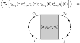
Figure 2: Graphical representation of the general correlator involved in the Majorana decomposition of the $\mathcal{T}$-matrix Eq. (III.1) and Eq. (25). The shaded box indicates interaction processes between conduction electrons and Majorana fermions to all orders in perturbation theory.

where the box represents spin-spin interactions to all orders. Since there are three different Majorana fermions, in principle nine different correlators have to be expanded in perturbation theory, but in reality only a small number of independent correlation functions arise, as we will see. To show this, we define the following abbreviation for the response functions introduced in Fig. 2:

$$M(\tau)=\begin{pmatrix}\hphantom{-i}\langle\downarrow\eta_{1}\downarrow\eta_{1}\rangle&\hphantom{-}i\langle\downarrow\eta_{1}\downarrow\eta_{2}\rangle&\hphantom{-i}\langle\downarrow\eta_{1}\uparrow\eta_{3}\rangle\\ -i\langle\downarrow\eta_{2}\downarrow\eta_{1}\rangle&\hphantom{-i}\langle\downarrow\eta_{2}\downarrow\eta_{2}\rangle&-i\langle\downarrow\eta_{2}\uparrow\eta_{3}\rangle\\ \hphantom{-i}\langle\uparrow\eta_{3}\downarrow\eta_{1}\rangle&\hphantom{-}i\langle\uparrow\eta_{3}\downarrow\eta_{2}\rangle&\hphantom{-i}\langle\uparrow\eta_{3}\uparrow\eta_{3}\rangle\end{pmatrix},$$ (25)

which allow to write more compactly the $\mathcal{T}$-matrix:

$$T_{\uparrow}(\tau)=-\frac{J^{2}}{4}G_{\Phi}(\tau)\begin{pmatrix}1,&1,&1\end{pmatrix}\cdot M(\tau)\cdot\begin{pmatrix}1\\ 1\\ 1\end{pmatrix}.$$ (26)

In order to perform a leading-log calculation of the $\mathcal{T}$-matrix, we will use in what follows a RPA resummation with a single polarization bubble, owing to the fact that non-RPA diagrams (i.e. involving crossings) are higher orders in logarithmic singularities. In Fig. 3 this RPA expansion is shown for the response function entering the $\mathcal{T}$-matrix.

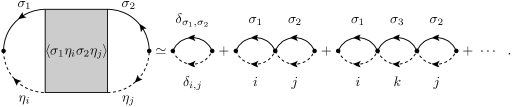
Figure 3: RPA-expansion of the response functions entering the $\mathcal{T}$-matrix in the Majorana language. The single polarization bubble involves the product of a free Majorana fermion propagator $G_{0\eta}$ and of a conduction electron propagator $G_{0c}$, and the RPA resummation corresponds to the leading logarithmic approximation of the standard one-loop renormalization procedure.

In the case of spin-rotation invariance, all the bubbles in Fig. 3 take the same value (given here in imaginary time):

$$\Pi_{0\eta}(\tau)=G_{0c}(\tau)G_{0\eta}(\tau).$$ (27)

Here the bare Majorana Green’s function simply read:

$$G_{0\eta}(i\omega)=\frac{1}{i\omega},$$ (28)

while the conduction electron propagator are given by:

$$G_{0c}(i\omega)=\sum_{\bm{k}}\frac{1}{i\omega-\epsilon_{\bm{k}}}.$$ (29)

The first terms in the diagrammatic series for the $\mathcal{T}$-matrix are easily checked to read:

$$\mathcal{T}_{\uparrow}(\tau)=\frac{J^{2}}{4}G_{\Phi}(\tau)\left[3\Pi_{0\eta}+\frac{J}{2}6\Pi_{0\eta}*\Pi_{0\eta}+\dots\right](\tau).$$ (30)

The factors $3$ and $6$ stem from equation (26), because at order $J^{2}$ the matrix $M$ in Eq. (25) is purely diagonal, while at order $J^{3}$ it is purely off-diagonal. The convolution operator in Eq. (30) is standardly defined as:

$$\frac{J}{2}\left[\Pi_{0\eta}*\Pi_{0\eta}\right](\tau)=\int_{0}^{\beta}\!\!\!\!\!d\tau_{1}\;\Pi_{0}(\tau-\tau_{1})\Pi_{0\eta}(\tau_{1})$$ (31)

We can already anticipate that a RPA-like resummation will be possible by Fourier transforming to imaginary frequencies. However, the numerical coefficient of the series (30) need to be obtained, and for this we will use a recursion based on the following diagrammatic rules. In principle, there are only two different response-functions. The first type is a response-function where the same Majorana fermion enters and leaves the interacting region (gray box of the $\mathcal{T}$-matrix in Fig. 3), or equivalently when no spin-flip of the conduction electrons occurs. These contributions are the diagonal terms of the matrix given in equation (25) and we call $a_{n}$ their combinatorial factor, so that they contribute in total to $3a_{n}$ to the $\mathcal{T}$-matrix in Eq. (26). The second type is a response-function where different Majorana fermions enter and leave the interacting region, so that the conduction electrons have flipped their spin. These processes are labeled with a combinatorial factor ${\color[rgb]{0,0,0}b_{n}}$ associated to the non-diagonal terms of the matrix in Eq. (25), thus contributing $6b_{n}$ to the $\mathcal{T}$-matrix, so that we have the general RPA-series:

$$\mathcal{T}_{\uparrow}(\tau)=\frac{3J^{2}}{4}G_{\Phi}(\tau)\sum_{n=0}^{\infty}({\color[rgb]{0,0,0}a_{n}}+2{\color[rgb]{0,0,0}b_{n}})\left(\frac{J}{2}\right)^{n}\underbrace{\left[\Pi_{0\eta}*\cdots*\Pi_{0\eta}\right]}_{(n+1)\operatorname{times}}$$ (32)

where $a_{0}=1,~{}b_{0}=0,~{}a_{1}=0$ and $b_{1}=1$. In order to find the explicit expression for $a_{n}$ and $b_{n}$, we note the combinatorics of Fig. 4 which follows from the fact that a Majorana fermion cannot scatter into itself, due to the identity $\eta_{a}^{2}=1/2$. Thus a diagonal process at order $n$ (described by $a_{n}$) results necessarily from a combination of all non-diagonal processes at order $n-1$ (described by $b_{n-1}$) and of a single off-diagonal term, for which two possibilities arise. This shows readily that $a_{n}=2b_{n-1}$. Similarly an off-diagonal process at order $n$ can be decomposed either by an arbitrary diagonal processes at order $n-1$ and a single off-diagonal one, or by all possible non-diagonal processes at order $n-1$ followed by a single non-diagonal one, so that $b_{n}=a_{n-1}+b_{n-1}$. We can trivially solve this recursion, and we find $a_{n}+2b_{n}=2^{n}$.

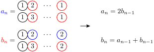
Figure 4: (color online) Combinatorics of the RPA diagrams at zero magnetic field: circles denote a single polarization bubble involving a Majorana fermion with flavor $1$,$2$, or $3$. The coefficient $a_{n}$ counts the number of possibilities at order $n$ to end up with the same index, while the coefficient $b_{n}$ counts the sequences with different head and tail. The mathematical recursion on the right side follows from this obvious pictorial description.

Using this result, the $\mathcal{T}$-matrix is given at RPA level by

$$\mathcal{T}_{\uparrow}(\tau)=\frac{3J^{2}}{4}G_{\Phi}(\tau)\Pi_{\eta}(\tau),$$ (33)

where $\Pi_{\eta}(\tau)$ is simply determined by a geometric series in Matsubara frequencies:

$$\Pi_{\eta}(i\nu)=\frac{\Pi_{0\eta}(i\nu)}{1-J\Pi_{0\eta}(i\nu)}.$$ (34)

We finally compute the expression for the $\mathcal{T}$-matrix, first by Fourier transforming to fermionic Matsubara frequencies:

$$\begin{split}\mathcal{T}_{\uparrow}(i\omega_{n})&=\frac{3J^{2}}{4}\frac{1}{\beta}\sum_{i\nu_{1}}G_{\Phi}(i\nu_{1})\Pi(i\omega_{n}-i\nu_{1})\\ &=\frac{3J^{2}}{8\pi}\int_{-\infty}^{\infty}\!\!\!\!d\omega_{2}\;\Pi^{{}^{\prime\prime}R}_{\eta}(\omega_{2})\frac{1+2n_{B}(-\omega_{2})}{\omega_{2}-i\omega_{n}},\end{split}$$ (35)

and using a spectral decomposition ($n_{B}$ is the Bose distribution). The analytic continuation is then straightforward, and we obtain the imaginary part of the real-frequency $\mathcal{T}$-matrix:

$$\mathcal{T}^{{}^{\prime\prime}R}_{\uparrow}(\omega)=-\frac{3J^{2}}{8}\coth\left(\frac{\beta\omega}{2}\right)\operatorname{Im}\left(\frac{\Pi^{R}_{0\eta}(\omega)}{1+J\Pi^{R}_{0\eta}(\omega)}\right)$$ (36)

with $\beta=1/T$ the inverse temperature. The polarization diagram $\Pi_{0\eta}$ is computed by similar means from Eq. (27) and reads for a flat conduction band with density of states $\rho_{0}=1/(2D)$ and half-bandwidth $D$:

$$\Pi_{0\eta}^{R}(\omega)=\frac{\rho_{0}}{2}\log\left(\left|\frac{\omega^{2}-D^{2}}{\omega^{2}}\right|\right)+i\pi\frac{\rho_{0}}{2}\operatorname{Sign}(\omega)\Theta(\omega^{2}-D^{2})$$ (37)

leading to the final result for $\mathcal{T}$-matrix at $T=0$:

$$-\pi\rho_{0}\mathcal{T}^{{}^{\prime\prime}R}_{\uparrow}(\omega)=\frac{3\pi^{2}}{16}\frac{(\rho_{0}J)^{2}\Theta(\omega^{2}-D^{2})}{\left(1-\frac{\rho_{0}J}{2}\log\left|\frac{D^{2}-\omega^{2}}{\omega^{2}}\right|\right)^{2}+\frac{\pi^{2}(\rho_{0}J)^{2}}{4}}.$$ (38)

Inserting this expression into the conductance formula (8), we recover the standard high-temperature result Eq. (12) for $T\gg T_{K}$. Let us contrast our expression to the standard weak-coupling renormalization group result in the case of antiferromagnetic Kondo exchange: $-\pi\rho_{0}\mathcal{T}^{{}^{\prime\prime}R}_{\uparrow}(\omega)=\frac{3\pi^{2}}{16}[\log(\omega/T_{K})]^{-2}$. In the range $T_{K}\ll\omega\ll D$, both are completely equivalent. For frequencies near the high energy cutoff $D$, the correct band-edge contribution appears in Eq. (38), which is usually neglected in the RG flow (but can be in principle incorporated). Stronger differences occur in the regime near and below $T_{K}$, where a maximum occurs in Eq. (38) instead of the usual divergence found in one-loop RG. The reason is the presence of a constant offset of order $J^{2}$ in the denominator, coming from the imaginary part of the Majorana bubble, which cuts off the Kondo singularity. This term shows that our RPA scheme picks not only the leading logarithms, but also some non-logarithmic terms in the perturbation series. The strong differences between one-loop RG and RPA at frequencies lower than $T_{K}$ appear however only in a regime where both theories are uncontrolled, and is thus of no physical significance. Indeed, we emphasize that perturbation theory still breaks down in our scheme for $\omega\ll T_{K}$, see Eq. (38), because the effective dimensionless Kondo coupling has reached values of order 1. Yet, the convergence of our result to NRG data for $\omega\simeq T_{K}$ seems slightly better than the lowest order RG expression, see Fig. 5, thanks to this partial resummation of subleading logarithmic terms. We now show how the Majorana diagrammatics can be extended to include the Zeeman effect as well.

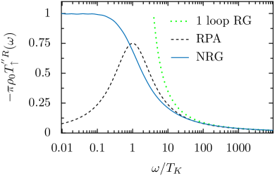
Figure 5: (color online) $\mathcal{T}$-matrix of the Kondo model with antiferromagnetic exchange at zero magnetic field, comparing the NRG simulations (full line) to the poor man’s scaling one-loop result (dotted line) and to the Majorana diagrammatics at RPA level (dashed line) given by Eq. (38).

III.3 Majorana diagrammatics at finite magnetic field

The Zeeman effect can be easily studied in quantum dots, by applying a magnetic field in the plane in the case of semiconducting two-dimensional electron gas devices. We note that the latter systems have relatively small $g$-factor, but because of the low Kondo temperature that they can achieve (in the range 100mK to 1K), a competition with the Kondo effect can occur at magnetic fields of a few Tesla. In molecular quantum dots larger $g\simeq 2$ values are obtained, which helps realizing the competition between Kondo and Zeeman effects. In this section, we simply add the Zeeman term to the Kondo Hamiltonian (1)

$$H_{Z}=BS^{z}=-iB\eta_{1}\eta_{2},$$ (39)

where $B$ is measured in units of the Zeeman splitting. We note that the Majorana fermion propagator $G_{ab}(\tau)$ has now non-diagonal elements, which makes it more difficult to carry out the previous RPA for the $\mathcal{T}$-matrix. The first idea is to transform the Majorana fermions so that their propagator becomes diagonal, which can be done by introducing one real fermion:

$$f^{\dagger}=\frac{1}{\sqrt{2}}(\eta_{1}+i\eta_{2}),~{}~{}~{}\left\{f^{\dagger},f\right\}=1.$$ (40)

The Kondo Hamiltonian is given after this transformation by:

$$\begin{split}H_{K}=&-\frac{J}{2}\sqrt{2}\left(c^{\dagger}_{0\downarrow}c^{\vphantom{\dagger}}_{0\uparrow}f^{\dagger}\eta^{\vphantom{\dagger}}_{3}+c^{\dagger}_{0\uparrow}c^{\vphantom{\dagger}}_{0\downarrow}\eta_{3}^{\dagger}f\right)\\ &+\frac{J}{2}\left(c^{\dagger}_{0\uparrow}f^{\dagger}fc^{\vphantom{\dagger}}_{0\uparrow}-c^{\dagger}_{0\downarrow}f^{\dagger}fc^{\vphantom{\dagger}}_{0\downarrow}\right)\\ &-\frac{J}{4}[c^{\dagger}_{0\uparrow}c^{\phantom{\dagger}}_{0\sigma\uparrow}-c^{\dagger}_{0\downarrow}c^{\phantom{\dagger}}_{0\sigma\downarrow}].\end{split}$$ (41)

The last term, corresponding to a small magnetic field acting on the bath of conduction electrons, is expected to remain perturbatively small. However, we will see in Sec. IV.3 that it needs to be kept in order to describe properly the self-energy in second order. The Zeeman term now becomes purely diagonal:

$$H_{z}=Bf^{\dagger}f-\frac{1}{2}B,$$ (42)

where the last term is only a constant and will be dropped from now on. Thus the transformation leads to two different fermionic propagators

$$G_{f}(i\omega_{n})=\frac{1}{i\omega_{n}-B},~{}~{}~{}G_{\eta_{3}}(i\omega_{n})=\frac{1}{i\omega_{n}},$$ (43)

where $G_{f}$ is a canonical fermion propagator and $G_{\eta_{3}}$ is the propagator of the unchanged Majorana fermion $\eta_{3}$. The label $3$ can be dropped and we will use in what follows $G_{\eta}$ as the Majorana fermion propagator. Next, the $\mathcal{T}$-matrix is expressed in terms $f$ and $\eta$:

$$\begin{split}\mathcal{T}_{\uparrow}(\tau)=&-\frac{J^{2}}{4}G_{\Phi}(\tau)\left(2{\color[rgb]{0,0,0}\langle\downarrow f\downarrow f^{\dagger}\rangle}+\sqrt{2}{\color[rgb]{0,0,0}\langle\downarrow f\uparrow\eta\rangle}\right.\\ &+\left.\sqrt{2}{\color[rgb]{0,0,0}\ \langle\uparrow\eta\downarrow f^{\dagger}\rangle}+\langle\uparrow\eta\uparrow\eta\rangle\right),\end{split}$$ (44)

We have now two different bare polarization bubbles $\Pi_{0f}$ and $\Pi_{0\eta}$, associated to $f$ and $\eta$ respectively, which are readily evaluated:

$$\Pi_{0\eta}(\omega) = \frac{\rho_{0}}{2}\log\left|\frac{D^{2}-\omega^{2}}{\omega^{2}}\right|+i\frac{1}{2}\pi\rho_{0}\operatorname{Sign}(\omega)$$ (45)

$$\Pi_{0f}(\omega) = \rho_{0}\log\left|\frac{D+B-\omega}{B-\omega}\right|+i\pi\rho_{0}\theta(\omega-B),$$ (46)

in the case $B>0$. Because of these two different contributions, the combinatorics cannot be guessed as easily as in the previous section, so we must use a more general resummation technique. The general structure of perturbation theory (with bare polarization bubbles) can be considered at the light of Fig. 6.

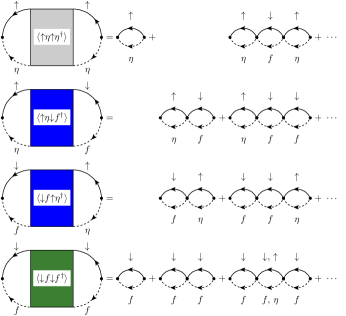
Figure 6: (color online) Lowest order contributions to the RPA evaluation of the $\mathcal{T}$-matrix in the case of finite magnetic field.

We introduce a dimensionful coefficient $A_{n}$ which encodes processes at order $n$ that start and finish with the bubble $\Pi_{0f}$, and a coefficient $B_{n}$ that involve $\Pi_{0f}$ and $\Pi_{0\eta}$ at its extremities. Note that these coefficients are not only combinatoric in character (like the coefficients $a_{n}$ and $b_{n}$ defined in the previous section), but also include a sum of terms of the type $[\Pi_{0f}]^{p}[\Pi_{0\eta}]^{n-p}$ with integer $p$, due to the fact that we have two independent polarization bubbles now. The correlations appearing in Eq. (44) are then expressed as:

$$\begin{split}&\langle\uparrow\eta\uparrow\eta\rangle=\Pi_{0\eta}+2\left(\frac{J\Pi_{0\eta}}{2}\right)^{2}\sum_{n=0}^{\infty}A_{n}\left(\frac{J}{2}\right)^{n}\\ &2\langle\downarrow f\downarrow f^{\dagger}\rangle=2\sum_{n=0}^{\infty}A_{n}\left(\frac{J}{2}\right)^{n}\\ &\sqrt{2}\left(\langle\uparrow\eta\downarrow f^{\dagger}\rangle+\langle\downarrow f\uparrow\eta\rangle\right)=2\sqrt{2}\sum_{n=0}^{\infty}B_{n}\left(\frac{J}{2}\right)^{n}\end{split}$$ (47)

so that the complete RPA series (44) for the $\mathcal{T}$-matrix reads:

$$\begin{split}T^{{}^{\prime\prime}R}_{\uparrow}(\omega)&=-\frac{J^{2}}{8}\coth\left(\frac{\beta\omega}{2}\right)\Pi^{{}^{\prime\prime}R}(\omega)\\ \Pi^{R}(\omega)=&\Pi_{0\eta}^{R}(\omega)+2\sum_{n=0}^{\infty}\left(\frac{J}{2}\right)^{n}\Bigg{\{}A_{n}+\left(\frac{J\Pi_{0\eta}^{R}(\omega)}{2}\right)^{2}A_{n}\\ &+\sqrt{2}B_{n}\Bigg{\}}.\end{split}$$ (48)

A recursion is easily established on the basis of Fig. 7, which can be best cast and solved in matrix form:

$$\begin{split}\begin{pmatrix}A_{n}\\ B_{n}\end{pmatrix}&=\begin{pmatrix}\Pi_{0f}&\sqrt{2}\Pi_{0f}\\ \sqrt{2}\Pi_{0\eta}&0\\ \end{pmatrix}\cdot\begin{pmatrix}A_{n-1}\\ B_{n-1}\end{pmatrix}\\ &=\begin{pmatrix}\Pi_{0f}&\sqrt{2}\Pi_{0f}\\ \sqrt{2}\Pi_{0\eta}&0\\ \end{pmatrix}^{n}\cdot\begin{pmatrix}A_{0}\\ B_{0}\end{pmatrix}\\ \end{split}$$ (49)

with $A_{0}=\Pi_{0f}$ and $B_{0}=0$ as can be inferred from the lowest order perturbative expansion shown in Fig. 6,

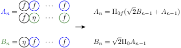
Figure 7: (color online) Combinatorics of the RPA diagrams at finite magnetic field: circles denote a single polarization bubble involving a real fermion $f$ or a Majorana $\eta$. The coefficient $A_{n}$ picks the contributions at order $n$ that end up with the same index $f$, while the coefficient $B_{n}$ collects the sequences with different head and tail. The mathematical recursion on the right side follows from this obvious pictorial description.

Inserting Eq. (49) into the expression (48) for the $\mathcal{T}$-matrix, we end up with the final compact result at zero temperature:

$$T^{{}^{\prime\prime}R}_{\uparrow}(\omega)=-\frac{J^{2}}{8}\operatorname{Sign}(\omega)\operatorname{Im}\left(\frac{\Pi_{0\eta}+2\Pi_{0f}+\frac{3}{2}J\Pi_{0f}\Pi_{0\eta}}{1-\frac{J}{2}\Pi_{0f}-\frac{J^{2}}{2}\Pi_{0\eta}\Pi_{0f}}\right)$$ (50)

which will be investigated in Sec. IV. If we take the limit $B\to 0$ before the limit of zero temperature, we find $\Pi_{0\eta}=\Pi_{0f}$, so that expression (50) reduces to

$$\begin{split}T^{{}^{\prime\prime}R}_{\uparrow}(\omega)&=-\frac{J^{2}}{8}\operatorname{Sign}(\omega)\operatorname{Im}\left(\frac{3\Pi_{0\eta}\left(1+\frac{J}{2}\Pi_{0\eta}\right)}{\left(1-J\Pi_{0\eta}\right)\left(1+\frac{J}{2}\Pi_{0\eta}\right)}\right)\\ &=-\frac{J^{2}}{8}\operatorname{Sign}(\omega)\operatorname{Im}\left(\frac{3\Pi_{0\eta}}{1-{J}\Pi_{0\eta}}\right)\end{split}$$ (51)

which is exactly the one established previously in Eq. (36) for zero magnetic field. Note however that the limit $B\to 0$ and $T\to 0$ clearly do not commute by comparing Eq. (45-46) and Eq. (37), due to the abrupt change in the ground state degeneracy of the free impurity spin as soon as a small magnetic field is turned on. At zero magnetic field, one can check that the expansions using a spin rotation-invariant formalism or a symmetry-broken one provide equivalent results for the physical observables (at $B=0$), such as the total $\mathcal{T}$-matrix $[\mathcal{T}^{R}_{\uparrow}+\mathcal{T}^{R}_{\downarrow}]/2$.

IV Results

In this section we investigate the analytic expressions obtained previously, both for antiferromagnetic and ferromagnetic exchange, and compare them to numerical renormalization group (NRG) calculations wilson_renormalization_1975 ; krishna-murthy_renormalization-group_1980 ; bulla_numerical_2008 . The simulations will be performed with the full density matrix using the DM-NRG algorithm hofstetter_generalized_2000 ; toth_density_2008 , which proved more accurate to compute observables in a finite (and possibly large) magnetic field compared to the standard NRG procedure.

IV.1 Anti-ferromagnetic Kondo model

The weak coupling RPA result Eq. (38) for the $\mathcal{T}$-matrix obtained at zero magnetic field can be rewritten in the limit $D\gg|\omega|\gg T_{K}$ in terms of the Kondo temperature $T_{K}$:

$$-\pi\rho_{0}\mathcal{T}^{{}^{\prime\prime}R}_{\uparrow}(\omega)\approx\frac{3\pi^{2}}{16}\frac{1}{\log^{2}\left|\frac{\omega}{T_{K}}\right|+\frac{\pi^{2}}{4}}.$$ (52)

This recovers the standard poor man’s scaling result, with some inclusion of high logarithmic corrections, which cut-off the divergence at $\omega=T_{K}$ (nevertheless, the RPA breaks down in this regime as well). This difference between the two results stems from the fact that the imaginary part of the polarization diagram is not neglected for the renormalization of Kondo exchange in the RPA. A benchmarking of this expression to the DM-NRG calculation was already provided in Fig. 5.

We now concentrate on the case of a finite magnetic field, where the presence of two scales, $\omega$ and $B$, prevent a simple poor man’s scaling, and requires more sophisticated analytical renormalization group techniques rosch_spectral_2003 ; rosch_kondo_2005 . Our result Eq. (50) obtained with the Majorana can be re-expressed in the regime $D\gg\omega\gg B$ or $-D\ll\omega\ll B$ as:

$$\begin{split}-\pi\rho_{0}\mathcal{T}^{{}^{\prime\prime}R}_{\uparrow}(\omega)\approx&\pi^{2}\frac{5}{16\log^{2}\left(\left|\frac{\omega}{T_{K}}\right|\right)}~{}~{}~{}~{}\mathrm{for}\;\hphantom{-}D\gg\omega\gg B\\ -\pi\rho_{0}\mathcal{T}^{{}^{\prime\prime}R}_{\uparrow}(\omega)\approx&\pi^{2}\frac{1}{16\log^{2}\left(\left|\frac{\omega}{T_{K}}\right|\right)}~{}~{}~{}~{}\mathrm{for}\;-D\ll\omega\ll B\end{split}$$ (53)

resulting in different asymptotes in the case of large positive and negative frequencies, in agreement with the fRG results by Rosch et al. rosch_spectral_2003 ; rosch_kondo_2005 . A global view on the the $\mathcal{T}$-matrix is given in Fig. 8, which shows a resonance that is now centered at $\omega=B$.

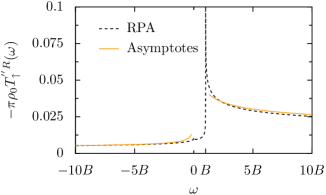
Figure 8: (color online) Spin-resolved $\mathcal{T}$-matrix of the Kondo model with antiferromagnetic exchange in a finite magnetic field $B=5000T_{K}$ as computed in the Majorana diagrammatics at RPA level from Eq. (50). The high energy asymptotes given in Eq. (53) are also shown. A remanence of the Kondo peak occurs for frequencies near $\omega=B$, see details in Fig. 9.

Note that perturbation theory is adequate because the scattering process remains far away from the unitary limit, $-\pi\rho_{0}\mathcal{T}^{{}^{\prime\prime}R}(\omega)\ll 1$.

Let us now consider the analytical results in more detail, by comparing them to DM-NRG simulations. For all the NRG calculations, we take the half bandwidth $D=1$ and the Kondo coupling $J/D=0.145$, so that the Kondo temperature is $T_{K}/D\simeq 10^{-6}$. All results will be obtained using the $U(1)$ symmetry and keeping the first 320 states, using a logarithmic discretization of the band with NRG parameter $\Lambda=2$. We consider also the standard broadening parameter $b$ in the range 0.5 to 0.9, in order to check possible problems of convergence in the broadening method (which can arise especially near the resonance at $\omega=B$). Fig. 9 shows the comparison of the NRG calculation and the analytical expression Eq. (50) for the $\mathcal{T}$-matrix.

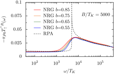
Figure 9: (color online) Close up on the finite magnetic field resonance in the Kondo model with antiferromagnetic exchange. This is a comparison between Majorana diagrammatics at RPA level (dashed line) and DM-NRG simulations with decreasing broadening parameter $b=0.85,0.75,0.65,0.55$ (solid lines, top to bottom) for a ratio $B/T_{K}=5000$. The NRG data are clearly overbroadened for frequencies near the threshold $\omega=B$. One note also a slight overshoot of the Majorana result at low frequency, also visible in Fig. 8, an artifact which is discussed in the text. In all other frequency ranges, the agreement between analytics and numerics is quantitative.

Clearly the agreement is overall excellent, but let us discuss rather the nature of the visible discrepancies. The most evident disagreement occurs near the resonance at $\omega=B$, where the NRG shows a very broad shoulder while the Majorana result at RPA level presents a threshold followed by a spurious logarithmic divergence. The study of several broadening parameters in Fig. 9 shows that the broadening of the NRG data converges well except near the resonance, so that the actual result is likely to display a threshold-like feature at $\omega=B$ similar to the Majorana result. This broadening issue of the NRG is a notoriously difficult problem, to which more refined broadening methods oliveira_generalized_1994 ; freyn_optimal_2009 do not bring much improvement Florens_spinboson ; Weichselbaum_Bfield . In contrast to this dynamically generated resonance of the $\mathcal{T}$-matrix, atomic like resonances (which occur in the abssence of dissipative coupling to the electronic environment) can be tackled by improved broadening method freyn_optimal_2009 ; Florens_spinboson ; Florens_Review , as we will see in Sec. IV.3 for the transverse spin susceptibility. Despite this flaw of the NRG to predict a threshold at $\omega=B$, the NRG simulation predict correctly a finite amplitude peak above the threshold, while the Majorana diagrammatics leads to a spurious logarithmic divergence at $\omega\to B^{+}$, which can be clearly traced back to the form of the $f$-fermion bubble in Eq. (46). It has been argued in the context of fRG rosch_spectral_2003 ; rosch_kondo_2005 that this spurious singularity should be smoothened by taking into account spin relaxation effects, an issue that we examine in Sec. IV.3.

A second drawback of the present RPA resummation scheme can be observed in the low frequency range in Figs. 8 and 9. While the plateau of the $\mathcal{T}$-matrix in the range $T_{K}\ll\omega\ll B$ is quantitatively reproduced by the Majorana diagrammatics, a spurious logarithmic divergence occurs at $\omega\ll T_{K}$, which leads to progressive deviations from the numerical results at lowering frequency. The origin of this behavior is easily understood from the Majorana fermion bubble Eq. (45), which displays an unbounded logarithm in the zero frequency limit. We have checked however that including spin relaxation effects will not cure this divergence, which has rather to do with deficiencies of the RPA resummation. Indeed, while the RPA diagrams reproduce exactly the one-loop poor man’s scaling approach at zero magnetic field, the RPA scheme at finite magnetic field is actually not fully equivalent to the fRG approach in the limit $\omega\ll T_{K}$ (the two approaches give however equivalent results otherwise). This difference can be understood from the fact that a one-loop renormalization of the Kondo exchange takes into accounts non-RPA diagram, such as seen in Fig. 10.

Figure 10: Upper panel: standard one-loop renormalization of the Kondo exchange. Resummation of the top right diagram (particle-hole channel) can be generalized in the Majorana diagrammatics in terms of the non-RPA extra contribution shown in the lower panel. The neglect of such terms which remain logarithmic in the range $\omega\ll T_{K}$ for finite magnetic field is the likely origin for the discrepancies of the RPA at low frequency (and finite $B$) with respect to one-loop fRG calculations.

One can check that these non-RPA diagram remain logarithmic in the range $\omega\ll T_{K}$ for finite magnetic field, and these will likely cancel out the spurious low frequency divergence of the RPA scheme (these diagrams are however logarithmically subdominant at high energy, allowing the good agreement between RPA and fRG for the other frequency regimes). We have unfortunately not been able to resum exactly to all orders the non-RPA diagram shown in the lower panel of Fig. 10. However, it is possible to put the present argumentation on a more precise ground, by noting that the leading contribution of the shown diagram in Fig. 10 is given by the combination $[\Pi_{0\eta}(\omega)]^{2}\Pi_{0f}(\omega=0)$. Iterating these terms in a geometric series to all orders amount to cancel the remaining spurious logarithmic divergence at low energy, as given by this new form of the $\mathcal{T}$-matrix:

$$T^{{}^{\prime\prime}R}_{\uparrow}(\omega) = -\frac{J^{2}}{8}\operatorname{Sign}(\omega)\times$$

$$\operatorname{Im}\left(\frac{\Pi_{0\eta}+2\Pi_{0f}+\frac{3}{2}J\Pi_{0f}\Pi_{0\eta}}{1-\frac{J}{2}\Pi_{0f}-\frac{J^{2}}{2}[\Pi_{0\eta}\Pi_{0f}-\Pi^{{}^{\prime}}_{0\eta}\Pi_{0f}(0)]}\right).$$

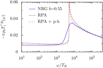
Figure 11: (color online) Kondo resonance in a finite magnetic field for antiferromagnetic exchange, with the same parameters as Fig. 9. This plot shows the corrected RPA with the approximate particle-hole channel (RPA+p-h) diagram of Eq. (IV.1), with comparison to NRG calculations and the uncorrected RPA.

Figure 11 shows indeed the elimination of the spurious low-$\omega$ resonance, and quantitative agreement with the NRG for all frequencies (except right at the threshold $\omega=B$). This successful benchmarking of the Majorana diagrammatics allows us to consider now with confidence the $\mathcal{T}$-matrix in the case of ferromagnetic exchange.

IV.2 Ferromagnetic Kondo model

We now turn to the central question of the present work, namely the magnetoconductance of the spin $S=1/2$ Kondo model with ferromagnetic exchange. This description also applies to the strong coupling limit of the spin $S=1$ underscreened Kondo model with antiferromagnetic exchange nozieres_kondo_1980 ; cragg_kondo_1978 , recently observed in molecular quantum dots roch_quantum_2008 ; roch_observation_2009 ; ParksUS . For both models, the ground state remains a spin doublet with logarithmic decoupling from the bath of conduction electrons, and so one expects an extreme sensitivity to an applied magnetic field.

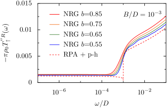
Figure 12: (color online) $\mathcal{T}$-matrix of the Kondo model with ferromagnetic exchange $J/D=-0.138$ and finite magnetic field $B/D=0.001$, comparing the DM-NRG calculations for broadening parameters $b=0.85,0.75,0.65,0.55$ (top to bottom) to the RPA result with particle-hole corrections Eq. (IV.1).

The ferromagnetic exchange modifies dramatically the flow equation of the Kondo coupling, which remains small at all energies, and even renormalizes to zero in the low frequency limit  cragg_kondo_1978 ; nozieres_kondo_1980 . We compare again the RPA results (with particle-hole corrections) with DM-NRG simulations, see Fig. 12. We find excellent agreement between the numerics and Majorana perturbation theory, as expected from the perturbative nature of the ferromagnetic Kondo model. However, near the resonance at $\omega=B$, one observes again that the DM-NRG results are overbroadened, similar to the antiferromagnetic case, so that the step predicted by the theory is difficult to reproduce. Perturbation theory displays also an artifact, as it predicts that the $\mathcal{T}$-matrix vanishes logarithmically at $\omega=B$, a behavior that will be corrected by including spin relaxation effects, see Sec. IV.3.

We finally address the issue of the Zeeman splitting in the spin-symmetric $\mathcal{T}$-matrix, see Fig. 13 which compares experimental results for a $S=1$ underscreened molecular quantum dot roch_observation_2009 and our analytical result. The analytical formula shows indeed that the Zeeman splitting persists for arbitrary small values of the applied magnetic field, giving strength to the interpretation made in Ref. roch_observation_2009, .

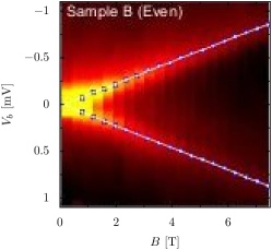
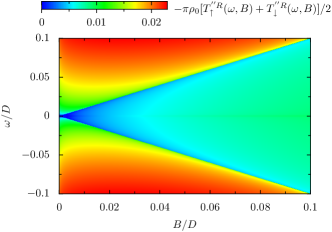
Figure 13: (color online) Upper panel: experimental data roch_observation_2009 for the finite bias conductance of an underscreened $S=1$ Kondo dot as a function of magnetic field and applied bias. A splitting is still observed at small magnetic field, below the typical voltage scale characterizing the width of the $B=0$ differential conductance. Lower panel: spin-symmetric $\mathcal{T}$-matrix of the $S=1/2$ Kondo model with ferromagnetic exchange ($J/D=-0.138$) as a function of magnetic field and frequency. Similarly to the experiment, the Zeeman effect persists even for vanishingly small magnetic field.

IV.3 Spin relaxation time

We finally investigate the role of spin relaxation in transport, motivated by the spurious logarithmic singularities obtained at RPA level in the $\mathcal{T}$-matrix near the threshold $\omega=B$. Following previous works rosch_spectral_2003 ; rosch_kondo_2005 ; Kehrein ; Schoeller ; Schuricht ; SchurichtAndergassen , one can expect that spin lifetime effects occuring at higher order in perturbation will smear out the artificial divergence of the $\mathcal{T}$-matrix. In the Majorana diagrammatics, spin relaxation is straightforwardly incorporated within Majorana self-energies, because the magnetic susceptibilities identically reduce to Majorana propagators, see e.g. Eq. (20).

Due to the presence of the magnetic field along the $z$-axis, we need to introduce longitudinal and transverse susceptibilities, $\chi_{z}(\tau)=-\left\langle T_{\tau}\left[S^{z}(\tau)S^{z}(0)\right]\right\rangle$ and $\chi_{\perp}(\tau)=-\left\langle T_{\tau}\left[S^{+}(\tau)S^{-}(0)\right]\right\rangle$. The spin operators are then replaced by $S^{z}=\Phi\eta$, $S^{+}=\sqrt{2}\Phi f^{\dagger}$ and $S^{-}=\sqrt{2}\Phi f$, so that imaginary parts of these susceptibilities are given by single fermion propagators:

$$\chi^{{}^{\prime\prime}R}_{z}(\omega) =-\frac{1}{2}\tanh\left(\frac{\beta\omega}{2}\right)G^{{}^{\prime\prime}R}_{\eta}(\omega)$$ (55)

$$\chi^{{}^{\prime\prime}R}_{\perp}(\omega) =-\tanh\left(\frac{\beta\omega}{2}\right)G^{{}^{\prime\prime}R}_{f}(\omega).$$ (56)

Spin relaxation is now immediately incorporated from Dyson’s equation:

$$G_{\eta}^{R}(\omega) = \frac{1}{\omega-\Sigma_{\eta}(\omega)+i0^{+}}$$ (57)

$$G_{f}^{R}(\omega) = \frac{1}{\omega-B-\Sigma_{f}(\omega)+i0^{+}}$$ (58)

and the needed imaginary part of the self-energies are easily computed up to second order in $J$ (here at zero temperature):

$$\Sigma_{\eta}^{{}^{\prime\prime}R}(\omega) = \delta\Sigma_{\eta}-\frac{J^{2}}{4}\rho_{0}\int_{-D}^{D}\left[\Pi_{0f}^{{}^{\prime\prime}R}(\omega_{1}+\omega)-\Pi_{0f}^{{}^{\prime\prime}R}(-\omega_{1}-\omega)\right]\left[\operatorname{Sign}(\omega_{1}+\omega)-\operatorname{Sign}(\omega_{1})\right]d\omega_{1}$$ (59)

$$\Sigma_{f}^{{}^{\prime\prime}R}(\omega) = -\frac{J^{2}}{4}\rho_{0}\int_{-D}^{D}\left[\Pi_{0f}^{{}^{\prime\prime}R}(\omega_{1}+\omega)+\Pi_{0\eta}^{{}^{\prime\prime}R}(\omega_{1}+\omega)\right]\left[\operatorname{Sign}(\omega_{1}+\omega)-\operatorname{Sign}(\omega_{1})\right]d\omega_{1},$$ (60)

from which the real part of the self-energies can be obtained by applying the Kramers-Kronig relation. The self-energy $\Sigma_{\eta}$ contains an extra $\omega$-independent contribution given by

$$\delta\Sigma_{\eta}=-\frac{J^{2}}{4}\int_{0}^{\beta}d\tau G_{0c}(\tau)G_{0c}(-\tau)=\frac{J^{2}}{4}\rho_{0}\log(4),$$ (61)

that originates from the last term in Eq. (41), and which is crucial to preserve the correct particle-hole symmetry. The susceptibilities obtained from the Majorana propagators (55)-(56) are shown in Figure 14.

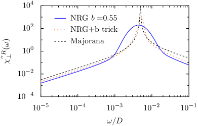
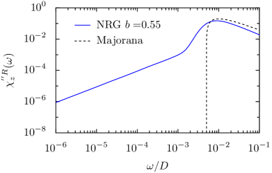
Figure 14: (color online) Upper panel: transverse spin susceptibility for the antiferromagnetic Kondo model, comparing the lowest order Majorana calculation to NRG simulations obtained with constant broadening bulla_numerical_2008 $b=0.55$ and with the adaptative broadening methods (“b-trick”) freyn_optimal_2009 , using the same parameters as in Fig. 9. The resonance at $\omega=B$ is clearly overbroadened, and the broadening trick allows to improve on the resolution. Lower panel: longitudinal spin susceptibility within the Majorana diagrammatics and the NRG (with constant broadening $b=0.55$ only). The spurious gap obtained by the lowest order diagrammatics result should be filled by enforcing self-consistency in the diagrammatic calculation scheme Florens_spinboson .

Let us begin with the discussion of the transverse susceptibility, which is expected to display a narrow resonance at the Zeeman energy. As noted previously Florens_spinboson , the NRG data for the transverse spin susceptibility is much more overbroadened than the $\mathcal{T}$-matrix (which only shows a shoulder and not a peak), as can be gathered from the sharper feature found in the Majorana calculation. Some improvement of the NRG data processing can be obtained by using adaptative broadening methods (“b-trick”) freyn_optimal_2009 , where the broadening parameter $b$ is taken to be frequency-dependent. This allows to obtain a much narrower peak, yet still somewhat too broad. Larger scale NRG simulations using so-called $z$-averaging oliveira_generalized_1994 should allow to obtain better agreement. We now turn to the longitudinal susceptibility, which similarly to the $\mathcal{T}$-matrix is expected Florens_spinboson to give a shoulder at $\omega=B$. The lowest order Majorana calculation shows good agreement with the NRG at $\omega>B$, but fails to reproduce the low-frequency tails, because the self-energy Eq. (60) has a gap. Previous work Florens_spinboson showed however that enforcing self-consistency in the perturbative scheme allows to cure this defect of the bare perturbation theory. Note also that the use of self-consistency in the self-energies allows to include the renormalization of the exchange coupling within the relaxation rate, a small quantitative effect that we did not take into account here.

Ultimately, it is the finite amplitude of the resonance peak in the spin susceptibilities at $\omega=B$ which is expected to regularize the spurious divergence in the $\mathcal{T}$-matrix rosch_spectral_2003 ; rosch_kondo_2005 ; Kehrein ; Schoeller ; Schuricht ; SchurichtAndergassen . This is simply achieved by replacing the free propagators Eq. (43) by the dressed ones Eq. (57)-(58) into the previous $\mathcal{T}$-matrix calculation. Figure 15 shows the inclusion of spin relaxation effects at the RPA level for the $\mathcal{T}$-matrix for the ferromagnetic Kondo model.

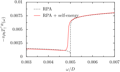
Figure 15: (color online) $\mathcal{T}$-matrix of the ferromagnetic Kondo model near the Zeeman energy $B=0.005D$, comparing the RPA calculation with and without self-energy corrections. The inclusion of a finite spin relaxation rate allows to cut the singularity (a spurious logarithmic vanishing at $\omega=B$) of the bare Majorana calculation.

The previously observed artifact, namely a logarithmic cancellation of $\mathcal{T}^{{}^{\prime\prime}R}$ at $\omega=B$, is now cured by the spin lifetime. Note still that the shoulder at the Zeeman energy persists, an important check to argue about the occurrence of a split Kondo resonance at low magnetic field in the underscreened situation roch_observation_2009 .

V Conclusion

The goal of this paper was to understand quantum transport under an applied magnetic field in presence of a ferromagnetic Kondo interaction. Although magnetic impurities (or spin-active quantum dots) are most often coupled antiferromagnetically to conducting electrons (see however Ref. lucignano_kondo_2009, ), the ferromagnetic case is relevant for the situation of underscreened large magnetic moments roch_observation_2009 ; ParksUS . Indeed, partially screened moments decouple weakly from the electrons at low energy, due to an effective ferromagnetic Kondo interaction nozieres_kondo_1980 . The existence of a degenerate magnetic ground state leads then to a singular response to magnetic field, also visible in transport, which we investigated here in some detail, using a combination of density-matrix numerical renormalization group calculations and an analytical perturbative technique based on Majorana diagrammatics Florens_spinboson . This latter method is conceptually simpler than previously proposed various renormalization scheme, either based on Callan-Symanzik equations Fritz , functional RG rosch_spectral_2003 ; rosch_kondo_2005 , flow equations Kehrein , and Liouvillian-based RG Schoeller ; Schuricht ; SchurichtAndergassen . However we have to recognize that the Majorana diagrammatics is likely harder to implement beyond one-loop, because disentangling the sub-leading logarithmic contributions really requires an RG method (the Majorana scheme performs yet very well beyond one loop near a perturbatively-accessible quantum critical point Florens_spinboson ). Another issue addressed here and in previous works rosch_spectral_2003 ; rosch_kondo_2005 is the energy resolution of the NRG, which is clearly insufficient. We believe that a careful comparison of large scale NRG simulations freyn_optimal_2009 ; Weichselbaum_Bfield ; Zitko and possibly two-loop RG analytics Schoeller ; Schuricht ; SchurichtAndergassen , already in the equilibrium situation, still need to be performed.

- (1) M. A. Kastner, Rev. Mod. Phys. 64, 849 (1992).
- (2) M. A. Kastner, Ann. Phys. 9, 885 (2000).
- (3) N. Roch, S. Florens, V. Bouchiat, W. Wernsdorfer, and F. Balestro, Nature 453, 633 (2008).
- (4) S. Florens, A. Freyn, N. Roch, W. Wernsdorfer, F. Balestro, P. Roura-Bas, and A. A. Aligia, J. Phys. Condens. Matter 23, 243202 (2011).
- (5) K. Kaasbjerg, and K. Flensberg, Nano Lett. 8, 3809 (2008).
- (6) J. V. Holm, H. I. Jorgensen, K. Grove-Rasmussen, J. Paaske, K. Flensberg and P. E. Lindelof, Phys. Rev. B 77, 161406(R) (2008).
- (7) J. R. Hauptmann, J. Paaske and P. E. Lindelhof, Nature Physics 4 373 (2008).
- (8) A. C. Hewson, The Kondo Problem to Heavy Fermions (Cambridge University Press, 1997).
- (9) D. Goldhaber-Gordon, H. Shtrikman, D. Mahalu, D. Abusch-Magder, U. Meirav, and M. A. Kastner, Nature 391, 156 (1998).
- (10) S. M. Cronenwett, T. H. Oosterkamp and L. P. Kouwenhoven, Science 281, 540 (1998).
- (11) M. Pustilnik and L. I. Glazman, J. Phys. Condens. Matter 16, R513 (2004).
- (12) M. Grobis, I. G. Rau, R. M. Potok and D. Goldhaber-Gordon, Kondo Effect in Mesoscopic Quantum Dots, Handbook of Magnetism and Magnetic Materials (Wiley, 2007).
- (13) N. Roch, S. Florens, T. A. Costi, W. Wernsdorfer, and F. Balestro, Phys. Rev. Lett. 103, 197202 (2009).
- (14) J. J. Parks, A. R. Champagne, T. A. Costi, W. W. Shum, A. N. Pasupathy, E. Neuscamman, S. Flores-Torres, P. S. Cornaglia, A. A. Aligia and C. A. Balseiro, G. K.-L. Chan, H. D. Abruña and D. C. Ralph, Science 328, 1370 (2010).
- (15) P. Nozières and A. Blandin, J. Phys. 41, 19 (1980).
- (16) P. Mehta, N. Andrei, P. Coleman, L. Borda, and G. Zaránd Phys. Rev. B 72, 014430 (2005).
- (17) W. Koller, A. C. Hewson, and D. Meyer, Phys. Rev. B 72, 045117 (2005).
- (18) D. E. Logan, C. J. Wright and M. R. Galpin, Phys. Rev. B 80, 125117 (2009).
- (19) A. Rosch, T. A. Costi, J. Paaske, and P. Wölfle, Phys. Rev. B 68, 014430 (2003).
- (20) A. Rosch, J. Paaske, J. Kroha, and P. Wölfle, J. Phys. Soc. Jap. 74, 118 (2005).
- (21) H. Schoeller, Eur. Phys. J. Special Topics 168, 179 (2009).
- (22) D. Schuricht, and H. Schoeller, Phys. Rev. B 80, 075120 (2009).
- (23) C. B. M. Hörig, D. Schuricht, and S. Andergassen, preprint arXiv:1110.6103.
- (24) P. Fritsch and S. Kehrein, Phys. Rev. B 81, 035113 (2010).
- (25) O. Parcollet and C. Hooley, Phys. Rev. B 66, 085315 (2002).
- (26) A. Shnirman and Y. Makhlin, Phys. Rev. Lett. 91, 207204 (2003).
- (27) W. Mao, P. Coleman, C. Hooley, and D. Langreth, Phys. Rev. Lett. 91, 207203 (2003).
- (28) L. N. Bulaevskii, M.Hruška, and G. Ortiz, Phys. Rev. B 68, 125415 (2003).
- (29) S. Florens, A. Freyn, D. Venturelli, and R. Narayanan, Phys. Rev. B 84, 155110 (2011).
- (30) M. Cabrera Cano, Zeeman splitting of the Kondo resonance in high magnetic fields, Master’s thesis, Karlsruher Institut für Technologie, (2011).
- (31) W. Hofstetter, Phys. Rev. Lett. 85, 1508 (2000).
- (32) A. I. Tóth, C. P. Moca, Ö. Legeza, and G. Zaránd, Phys. Rev. B 78, 245109 (2008).
- (33) K. G. Wilson, Rev. Mod. Phys. 47, 773 (1975).
- (34) H. R. Krishna-murthy, J. W. Wilkins, and K. G. Wilson, Phys. Rev. B 21, 1003 (1980).
- (35) R. Bulla, T. A. Costi, and T. Pruschke, Rev. Mod. Phys. 80, 395 (2008).
- (36) P. Lucignano, R. Mazzarello, A. Smogunov, M. Fabrizio, and E. Tosatti, Nature Mat. 8, 563 (2009).
- (37) G. D. Mahan, Many-Particle Physics, (Springer, 1990).
- (38) H. Bruus and K. Flensberg, Many-body quantum theory in condensed matter Physics, (Oxford University Press, 2004).
- (39) M. Pustilnik and L. I. Glazman, Phys. Rev. B 64, 045328 (2001).
- (40) L. Borda, L. Fritz, N. Andrei, and G. Zaránd, Phys. Rev. B 75, 235112 (2007).
- (41) P. Coleman, preprint arXiv:cond-mat/0206003v3 (2002).
- (42) R. D. Mattuck, A Guide to Feynman Diagrams in the Many-Body Problem, (Dover, 1992).
- (43) W. C. Oliveira and L. N. Oliveira, Phys. Rev. B 49, 11986 (1994).
- (44) A. Freyn and S. Florens, Phys. Rev. B 79, 121102 (2009).
- (45) A. Weichselbaum, F. Verstraete, U. Schollwöck, J. I. Cirac and J. von Delft, Phys. Rev. B 80, 165117 (2009).
- (46) D. M. Cragg and P. Lloyd, J. Phys. C: Sol. State Phys. 12, 215 (1978).
- (47) L. Fritz, S. Florens, and M. Vojta, Phys. Rev. B 74, 144410 (2006).
- (48) R. Zitko, Phys. Rev. B 84, 085142 (2011).