A computationally efficacious free-energy functional
for studies of inhomogeneous liquid water

Abstract

We present an accurate equation of state for water based on a simple microscopic Hamiltonian, with only four parameters that are well-constrained by bulk experimental data. With one additional parameter for the range of interaction, this model yields a computationally efficient free-energy functional for inhomogeneous water which captures short-ranged correlations, cavitation energies and, with suitable long-range corrections, the non-linear dielectric response of water, making it an excellent candidate for studies of mesoscale water and for use in ab initio solvation methods.

I Introduction

The emergence of several macroscopic phases of water with distinct microscopic structures IceReview ; AmorphousIceReview from relatively simple molecular interactions places this liquid at the forefront of interesting unsolved problems in the study of condensed matter. The structure of water around microscopic objects differs significantly from the bulk,ConfinedWater and such effects play a critical role in the structure of proteins WaterProteinFolding and in chemical reactions at catalyst surfaces.WaterCatalyst

Current computational approaches to systems sensitive to liquid structure most often employ molecular dynamics simulations. Ab initio molecular dynamics,CPMD which treats all the valence electrons in the system quantum mechanically, is relatively accurate but prohibitively expensive for all but the smallest of systems. Hybrid approaches that combine electronic structure methods for part of the system with classical molecular dynamics simulations for the fluid can handle larger systems, but require empirical models for both the electron-fluid coupling and the classical pair potentials for the fluid. These molecular dynamics methods are inherently expensive due to the sampling required for thermodynamic averages which, when coupled to an electronic system, necessitates repeated electronic structure calculations. In addition, the thermodynamic integration required to calculate free energies, which are necessary for analyzing chemical reaction pathways, significantly exacerbates the cost of such methods.

Efficient theories for the equilibrium properties of liquids, on the other hand, deal directly with average densities instead of individual molecular configurations. Integral equation theories give accurate structures of inhomogeneous fluids,IntEqnInhomogeneous but still prove relatively expensive, particularly for estimating free energies. The most direct approach to free energies is classical density-functional theory, a method based on approximations to the exact free-energy functional of the liquid,MerminTheorem which has the added advantage of being readily coupled to electronic density-functional theory within the framework of joint density-functional theory.JDFT The most accurate, currently available functionals for polar molecular fluids such as water,WDA ; WaterFreezingDFT ; LischnerHCl ; LischnerH2O ; WuIntegralEqnCDFT however, rely on direct correlations (from neutron scattering or computer simulation) at each temperature and pressure of interest, restricting their efficiency and applicability.

This work addresses the need for a computationally efficacious microscopic theory of water that is capable of providing accurate free energies under inhomogeneous conditions without the dependence on fluid structure data. The strategy is to identify a simple effective microscopic Hamiltonian which (a) reproduces the equation of state for homogeneous water and (b) is readily represented by a free-energy functional even in the inhomogeneous case.

Statistical Associating Fluid Theory,SAFT-DFT based on Wertheim’s thermodynamic pertubation theory,WertheimTPT is one such approach which has been successfully applied to the study of vapor-liquid interfaces,SAFT-Tension with model parameters for water determined from the equation of state.SAFT-Water However, the predictions of this theory for the inhomogeneous fluid have not yet included quantities of interest in solvation methods such as pair correlations, cavitation energies and dielectric response, partly due to the relative complexity of the model Hamiltonian. Below, we develop an alternate simpler Hamiltonian based upon microscopic intuition about hydrogen bonding, and we demonstrate that the resulting functional (also based on Wertheim theory) leads to a relatively accurate free-energy description of inhomogeneous water, especially given the simplicity of the underlying model.

II Model molecular Hamiltonian and the equation of state for water

Within the constraints of condition (b) above, a natural starting point would be the standard approach of perturbation about the hard-sphere fluid, for which Fundamental Measure TheoryRosenfeldFMT ; TarazonaFMT ; WhiteBearFMT_MarkII ; FMTreview provides a highly accurate functional. The hard-sphere diameter required to reproduce bulk properties can be inferred from the excluded volume in the equation of state, and fitsJeffAustinEOS to experimental data suggest a value that strongly decreases with temperature and is $\sim 3.3$Å at $298$ K. This is clearly incompatible with the almost temperature-independent $\sim 2.8$Å location of the first peak in the experimentally observed oxygen-oxygen radial distribution.SoperEPSR

This incompatibility stems from the discrepancy between the close-packed coordination of the hard-sphere fluid and the tetrahedral coordination favored by water. Water prefers the formation of open tetrahedral networks at lower temperatures, which leads to empty space, “voids”, within cages of water molecules, as manifested by the temperature-dependent excess excluded volume in the equation of state. Consequently, we propose a reference fluid consisting of a compound object (FIG. 1(a)): a hard sphere of radius $R_{O}$ at the $O$ (oxygen) site with smaller spheres of radii $R_{V}$ at two void sites $V$ placed in contact (at a distance $\sigma_{OV}=R_{O}+R_{V}$) along two of the conjugate tetrahedral directions to the hydrogen bond directions. For our model, we take the $O$-$H$ distance to be 1 Å with a tetrahedral $H$-$O$-$H$ angle, as in the frequently employed SPC/E interatomic potential model.SPCE The geometry of this compound object is chosen to encourage closest approach along the hydrogen bond directions.

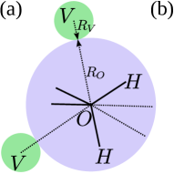
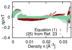
Figure 1: (a) Tangentially bonded hard-sphere model for liquid water: $O$ (oxygen) sphere with two $V$ spheres in contact diametrically opposite to the $H$ (hydrogen) sites (b) Residual for the equation of state (1) fit to experimental data,BulkData ; SupercooledData compared to the semi-empirical Jeffery-Austin equation of state.JeffAustinEOS

Our ansatz for the intermolecular Hamiltonian is the repulsive pair potential corresponding to the tangentially bonded hard-sphere trimer of FIG. 1(a), perturbed by an isotropic attractive pair potential $U_{a}(r)$ between the $O$ sites. The equation of state of this fluid is well approximated by

$$p(n,T) =p_{\textrm{id}}+p^{\textrm{ex}}_{\textrm{HS}}-2n^{2}T\left.\frac{\partial\log\left.g^{\textrm{HS}}_{OV}\right|_{\sigma_{OV}}}{\partial n}\right|_{T}-\frac{\kappa n^{2}}{2},$$ (1)

where the first three terms correspond to the bonded hard-sphere equation of state,BHS_EOS and the final term is the mean-field contribution from the as yet undetermined attractive perturbation $U_{a}(r)$, with $\kappa\equiv-\int\textrm{d}r4\pi r^{2}U_{a}(r)$.

The bonded hard sphere equation of state is based on Wertheim perturbation theory WertheimTPT about the hard sphere mixture, consisting of density $n$ of $O$-spheres and $2n$ of $V$-spheres. The pressure of this reference system is $p_{\textrm{HS}}=3nT+p^{\textrm{ex}}_{\textrm{HS}}$, where we separate and collect the $\mathcal{O}(n)$ ideal gas parts to elucidate the connection with the density functional (6). For $p^{\textrm{ex}}_{\textrm{HS}}$, we employ the accurate generalizationHardSphereEOS_CSIII of the Carnahan-Starling excess pressure to hard sphere mixtures

$$p^{\textrm{ex}}_{\textrm{HS}} =T\left[\frac{n_{0}n_{3}}{1-n_{3}}+\frac{n_{1}n_{2}}{(1-n_{3})^{2}}\left(1+\frac{n_{3}^{2}}{3}\right)\right.$$

$$+\left.\frac{n_{2}^{3}}{12\pi(1-n_{3})^{3}}\left(1-\frac{2n_{3}}{3}+\frac{n_{3}^{2}}{3}\right)\right],$$ (2)

where $n_{0}=3n$, $n_{1}=(R_{O}+2R_{V})n$, $n_{2}=4\pi(R_{O}^{2}+2R_{V}^{2})n$ and $n_{3}=\frac{4\pi}{3}(R_{O}^{3}+2R_{V}^{3})n$ are the uniform fluid fundamental measures.

First order Wertheim perturbation for the bonding constraints accounts for the fixed $O$-$V$ separation and not the $V$-$O$-$V$ angle; nonetheless it has been shown to well approximate the equation of state of objects with this geometry.BHS_EOS We accumulate its contribution at $\mathcal{O}(n)$ into the first term of (1): this exactly corrects the ideal gas mixture value of $3nT$ to the rigid-molecule ideal gas value of $p_{\textrm{id}}=nT$. (We use this fact later to restore the bond angle constraints in the intramolecular geometry of the inhomogeneous fluid.) The remaining contribution of this perturbation, the third term of (1), corrects the excluded volume effects of the hard sphere mixture to account for the $O$-$V$ distance constraints. There,

$$\left.g^{\textrm{HS}}_{OV}\right|_{\sigma_{OV}}=\frac{1}{1-n_{3}}+\frac{n_{2}R_{\textrm{hm}}}{(1-n_{3})^{2}}+\frac{2(n_{2}R_{\textrm{hm}})^{2}}{9(1-n_{3})^{3}},$$ (3)

is the contact value of the $O$-$V$ radial distribution in the hard sphere mixture with $R_{\textrm{hm}}=R_{O}R_{V}/\sigma_{OV}$.

As motivated earlier, the temperature dependence of the exclusion volume is a critical feature of the equation of state for water.JeffAustinEOS Because the location of the first peak in the $O$-$O$ radial distribution does not change appreciably with temperature, we attribute this dependence to changes in the radii of the $V$ spheres, modeled as a decreasing function $R_{V}(T)=R_{V}^{(0)}\textrm{e}^{-T/T_{V}}$ to qualitatively capture the effect of the empty spaces in the open tetrahedral network. This leads to a model equation of state (1) with only four adjustable parameters ($R_{V}^{(0)}$, $T_{V}$, $\kappa$, and $R_{O}$), which we fit to experimental data for the bulk liquid and vapor BulkData including data for the supercooled liquid.SupercooledData

The root mean-square error in the ratio of the pressure to the ideal-gas pressure, $p/nT$, is $4.8\times 10^{-2}$ for the current 4-parameter fit, which compares very favorably with $2.9\times 10^{-2}$ for the standard semi-empirical Jeffery-Austin equation of stateJeffAustinEOS (comparison in FIG. 1(b)), especially considering the fact that the latter fit employs more than twice as many ($\sim 9$) adjustable parameters. Beyond providing a reasonable fit to the equation of state, the key advantage of the present work is that these results stem directly from a model microscopic Hamiltonian, which we exploit below to construct a theory for the inhomogeneous fluid.

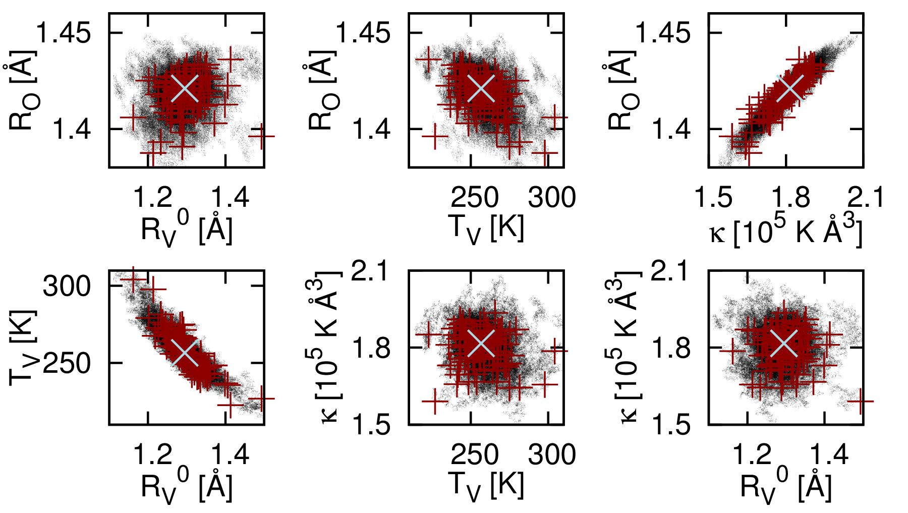
Figure 2: Metropolis sampling of a canonical ensemble of parameters, shown in all six projections of the four-dimensional parameter space. One hundred random samples ($+$) are drawn from the full set ($\cdot$) for error estimation of all subsequent results; $\times$’s mark the optimum parameter set.

To ensure that our model parameters are indeed independent and physically meaningful, we employ Bayesian error estimation following Ref.30,31. Specifically, we generate a canonical ensemble of parameter sets (FIG. 2) with a Metropolis walk in parameter space, where the residual is the ‘energy’ and the ‘temperature’ is $2C_{0}/N_{p}$ where $C_{0}$ is the minimum residual and $N_{p}=4$ is the number of fit parameters. The optimum parameters with standard deviations thus estimated are

$$R_{V}^{(0)} =(1.290\pm 0.049)\mbox{\AA}$$

$$T_{V} =(258.7\pm 12.3)K$$

$$\kappa =(1.805\pm 0.074)\times 10^{5}K\mbox{\AA}^{3}$$

$$R_{O} =(1.419\pm 0.010)\mbox{\AA}.$$ (4)

The modest eccentricities of the ensemble slices in FIG. 2 indicate that the covariances of these parameters are nominal, suggesting that the parameters have physical meaning rather than merely controlling a flexible fit function for the equation of state.

An advantage of this ensemble-of-models approach, which we exploit below, is that one can estimate how well the fit to bulk data constrains all subsequent predictions, including those for the inhomogeneous fluid, by evaluating those predictions for a sampling of the ensemble of parameters (indicated in FIG. 2 as +’s), instead of just the one optimum parameter set.

III Model for inhomogeneous liquid

Capturing the behavior of the inhomogeneous fluid requires information beyond merely the integrated strength $\kappa$ of the pair-potential interaction $U_{a}(r)$. This work demonstrates that the simplest next step, including information about the range of the interaction, suffices to capture surprisingly well the main features of the short-range correlations in the liquid. To this end, we employ the attractive-part of the Lennard-Jones potential

$$U_{a}(r)=\frac{-9\kappa}{8\pi\sqrt{2}\sigma_{U}^{3}}\left\{\begin{array}[]{lc}(\sigma_{U}/r)^{6}-(\sigma_{U}/r)^{12},&r\geq 2^{1/6}\sigma_{U}\\ 1/4,&r<2^{1/6}\sigma_{U}\end{array}\right.$$ (5)

which has the correct long range $r^{-6}$ tail for the orientation-averaged interaction of a dipolar fluid. We fit the range $\sigma_{U}$ to reproduce the bulk surface tension at $298$ K (based on calculations with the free-energy functional below), finding $\sigma_{U}=2.62$ Å. We thereby introduce only one additional fit parameter in going to the inhomogeneous fluid.

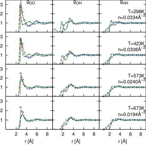
Figure 3: Partial radial distributions from the density functional (6) (bundle of thin red lines for the ensemble, with results for optimum parameters highlighted by dashed line) and Monte Carlo simulations for the model Hamiltonian (blue circles), compared to experimental pair correlations of water from Soper et al.SoperEPSR (green dot-dashed line)

To evaluate the viability of this simple model Hamiltonian for describing the inhomogeneous fluid, we compute its pair correlation functions (for each of the state points for which experimental correlations were measured in Soper et al.SoperEPSR ) directly with canonical-ensemble Monte Carlo simulations of 2048 molecules. The comparison (FIG. 3) between the behavior of this model microscopic Hamiltonian (circles) and the actual experimental correlations in physical water (green dash-dot line) is remarkable given the highly simplified form for the model. Although the secondary peaks in the $O$-$O$ correlations of this model Hamiltonian do appear more at the characteristic distances for a hard-sphere rather than at those for a tetrahedrally bonded fluid, the temperature and pressure dependence of the locations and heights of the first $O$-$O$ peak compare reasonably to water. Similarly, although the first two peaks of the $O$-$H$ and $H$-$H$ correlations are fused into a single broader peak, the general location and particle content of these peaks are in reasonable agreement for such a simple model. These details could be corrected in future work by fitting perturbation pair potentials of zero integral $\Delta U_{\alpha\beta}(r)$ with $\alpha,\beta\in\{O,H\}$ to the experimental correlation data, but the focus of the present work is the quality of predictions which can be made from a simple microscopic model with very few adjustable parameters (five) constrained purely by the macroscopic data.

Having established a short-ranged microscopic model Hamiltonian which reproduces relatively well the experimental correlations in water, we turn next to development of a corresponding free-energy functional. The form of this functional,

$$\Phi[\psi]=\Phi_{\textrm{id}}+\Phi^{\textrm{ex}}_{\textrm{HS}}+\Phi_{b}+\frac{1}{2}\int n_{O}\left(U_{a}\ast n_{O}\right),$$ (6)

mirrors the equation of state (1), and is composed of the ideal gas free energy, hard sphere excess functional, bonding correction and mean field perturbation.

We start with the exact grand free energy functional for the ideal gas of rigid molecules and thereby restore exact treatment of the intramolecular bond-angle constraints; this approach is consistent with Wertheim theory since the latter yields the exact rigid-molecular ideal gas pressure $p_{id}=nT$ at $\mathcal{O}(n)$ in the uniform limit. The free energy of the inhomogeneous ideal gas with chemical potential $\mu$ in external site potentials $V_{\alpha}(\vec{r})$ is written as

$$\Phi_{\textrm{id}}[\psi,n[\psi]]= \sum_{\alpha}\int d\vec{r}n_{\alpha}(\vec{r})(V_{\alpha}(\vec{r})-\psi_{\alpha}(\vec{r}))$$

$$-(\mu+T)\int d\vec{r}n_{O}(\vec{r}),$$ (7)

employing ideal gas effective potentials RISM1 ; RISM2 $\psi_{\alpha}(\vec{r})$ for $\alpha\in\{O,H,V\}$ as the sole independent variables.LischnerHCl Here, the site densities are dependent variables computed using

$$n_{\alpha}(\vec{r})=\frac{\delta}{\delta\psi_{\alpha}(\vec{r})}\int\frac{d\omega d\vec{r}^{\prime}}{4\pi^{2}}\exp\frac{-1}{T}\sum_{\alpha^{\prime},i}\psi_{\alpha^{\prime}}(\vec{r}^{\prime}+\omega\circ\vec{R}_{\alpha^{\prime}i}),$$ (8)

where $\omega\in SO(3)/\mathbb{Z}_{2}$, where $\omega\circ$ denotes the corresponding rotation for a vector, and where $\vec{R}_{\alpha i}$ are the site coordinates for a molecule in the reference orientation centered at the origin with $i=1$ for $\alpha=O$ and $i\in\{1,2\}$ for $\alpha\in\{H,V\}$. Note that we have simplified the above expression using the $\mathbb{Z}_{2}$ rotation symmetry of the molecule about its dipole axis.

To treat the hard sphere mixture excess free energy $\Phi^{\textrm{ex}}_{\textrm{HS}}$, we use the ‘White-Bear mark II’ version of fundamental measure theoryWhiteBearFMT_MarkII (incorporating Tarazona’s tensor modificationsTarazonaFMT )

$$\Phi^{\textrm{ex}}_{\textrm{HS}} =T\int\left[\begin{array}[]{c}n_{0}\log\frac{1}{1-n_{3}}+\frac{n_{1}n_{2}-\vec{n}_{v1}\cdot\vec{n}_{v2}}{1-n_{3}}f_{2}(n_{3})+\\ \frac{n_{2}^{3}-3n_{2}\vec{n}_{v2}^{2}+9\vec{n}_{v2}\bar{n}_{m2}\vec{n}_{v2}-\frac{9}{2}\textrm{Tr}\bar{n}_{m2}^{3}}{24\pi(1-n_{3})^{2}}f_{3}(n_{3})\end{array}\right],$$ (11)

in terms of the scalar, vector and tensor weighted densities $n_{i}=w_{i}^{O}\ast n_{O}+w_{i}^{V}\ast n_{V}$ for $i\in\{0,1,2,3,v1,v2,m2\}$, where

$$\begin{array}[]{rl}f_{2}(n_{3})&=1+\frac{n_{3}(2-n_{3})+2(1-n_{3})\log(1-n_{3})}{3n_{3}}\\ \textrm{and }f_{3}(n_{3})&=1-\frac{2n_{3}-3n_{3}^{2}+2n_{3}^{3}+2(1-n_{3})^{2}\log(1-n_{3})}{3n_{3}^{2}}.\end{array}$$

(See the comprehensive review by R. RothFMTreview for details.) Note that this functional corresponds exactly to the hard sphere excess pressure (2) in the uniform fluid limit.

Next, $\Phi_{b}$ accounts for the tangential bonding constraints on the hard-sphere exclusion effects; note that the contribution from Wertheim pertubation to the ideal gas part has been absorbed into the exact rigid-molecule ideal gas free energy $\Phi_{\textrm{id}}$. The Helmholtz-energy density for this term in the uniform fluid limit is determined from the third term of (1) to be $-2nT\log g^{\textrm{HS}}_{OV}(\sigma_{OV})$, which we generalize to the inhomogeneous version

$$\Phi_{b}=\int\frac{-2n_{0}T}{3}\log\left[\frac{1}{1-n_{3}}+\frac{\zeta n_{2}R_{\textrm{hm}}}{(1-n_{3})^{2}}+\frac{2\zeta n_{2}^{2}R_{\textrm{hm}}^{2}}{9(1-n_{3})^{3}}\right],$$ (13)

with the vector correction factor $\zeta=1-|\vec{n}_{v2}|^{2}/n_{2}^{2}$. We include this factor here following the spirit of Yu et al.,WuBonding where $\zeta$ was introduced in analogy with the occurence of the vector weighted densities in the hard sphere mixture functional in order to improve agreement with Monte Carlo calculations. Finally, the last term in (6) describes the attractive perturbation potential within a mean-field picture.

The partial radial distribution functions implied by the free energy functional (6), as evaluated from its analytic second variational derivatives using the Ornstein-Zernike relation, are in excellent agreement with the Monte Carlo simulations (circles and corresponding curve in FIG. 3). (The minor artifacts in the interior of the hard cores are caused by the bonding correction, whose inhomogeneous generalization is not perfect.) The small spread in these results with variation of parameters in the ensemble exemplifies how tightly the bulk data indeed constrain these predictions within the assumed model.

IV Predictions for the inhomogeneous liquid

To evaluate the predictions of the above density functional for the inhomogeneous fluid, we perform direct minimization of (6) using the nonlinear conjugate gradients algorithm NCG with the values of $\psi_{\alpha}(\vec{r})$ on a discretized grid as the independent variables. The orientation integrals involved in evaluating the site densities from the site potentials (8) are discretized using quadratures on $SO(3)/\mathbb{Z}_{2}$. The calculations presented below are performed on radial or planar $d=1$ dimensional grids Note2 where the azimuthal symmetry simplifies the orientation quadrature from $SO(3)\equiv\mathbb{S}_{2}\times\mathbb{S}_{1}$ to $\mathbb{S}_{2}$, which we tesselate using a recursively subdivided icosahedron. Note1

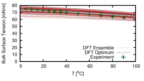
Figure 4: Energy of the vapor-liquid interface as a function of temperature, compared to the experimental values for surface tension.LangeHandbook

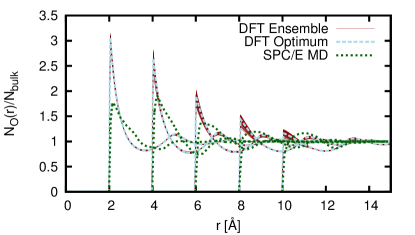
Figure 5: Comparison of density functional predictions with SPC/E molecular dynamics resultsHardSphereSPCE for (a) Radial distribution around spheres of radii 2, 4, 6, 8, and 10Å that exclude the oxygen sites and (b) the variation of solvation energy of such spheres per surface area with radius.

We find remarkable agreement with available data for the behavior and free energies of inhomogeneous aqueous systems, especially given that only bulk data, including surface tension at a single temperature, were employed in determining the limited number of parameters in the functional. For example, FIG. 4 compares our prediction of the temperature dependence of the interfacial energies with experimental data. Over the entire range of accessible temperatures at ambient pressure, we find the experiment to lie within the relatively narrow variations within our ensemble of models. Moving beyond planar interfaces, FIG. 5 explores the radial distribution around hard spheres and the variation of free energy of hard-sphere insertion with radius, and demonstrates that the predictions of our model are in qualitative agreement with the SPC/E molecular dynamics results. HardSphereSPCE The contact densities and the free energies from our model are somewhat higher than those from the SPC/E model results, a situation which could potentially be improved in future work by including additional perturbation pair-potentials.

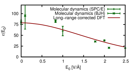
Figure 6: Nonlinear dielectric response: variation of relative dielectric constant $\epsilon$ with externally applied field $E_{0}$ at ambient conditions in comparison to SPC/ENonlinearEpsSPCE and BJHNonlinearEpsBJH molecular dynamics simulations. By construction, the linear dielectric constant matches experiment due to the long-range corrections.

In addition to the bulk and short-ranged correlations described above, a successful theory of solvation requires accurate dielectric response. Following Lischner et al.,LischnerH2O we add a scaled mean-field long range electrostatic correction

$$\Phi_{\epsilon}=\frac{A_{\epsilon}(T)}{2}\sum_{\alpha,\beta\in\{O,H\}}Z_{\alpha}Z_{\beta}\int n_{\alpha}K\ast n_{\beta},$$ (14)

where the site charges $Z_{\alpha}$ are taken to be the SPC/E values SPCE and $K\equiv\frac{4\pi}{G^{2}(1+(G/G_{c})^{4})}$ with $G_{c}=0.33$ is the Coulomb kernel with a high frequency (short range in space) cutoff LischnerH2O . The prefactor $A_{\epsilon}(T)=1-T/(7.35\times 10^{3}~{}\textrm{K})$ serves to correct for dipole correlations beyond mean field, and is fit to reproduce the bulk dielectric constant at small field. Fig. 6 shows that the nonlinear response at high fields (which is not fit) is well captured by the interplay between $\Phi_{\epsilon}$ and $\Phi_{\textrm{id}}$.

Conclusion — We have constructed a computationally tractable free-energy functional for studies of inhomogeneous water based upon a microscopic Hamiltonian constrained by experimental data for the bulk equation of state. Following this approach gives a remarkably high-quality fit to the equation of state with only four tightly constrained parameters. With one additional parameter, the range of the model interaction, the resulting functional captures the free energies associated with inhomogeneous systems such as the liquid-vapor interface and the embedding free energy of microscopic objects, as well as essential features of the partial radial distributions and density profiles around microscopic objects. With long-range corrections, the model gives an accurate description of the non-linear dielectric response. The model thus shows good promise for capturing the key quanties which require description in solvation studies. In future work, further details may be captured with suitable perturbation of the pair potentials constituting the underlying microscopic Hamiltonian.

This work was supported as a part of the Energy Materials Center at Cornell (EMC²), an Energy Frontier Research Center funded by the U.S. Department of Energy, Office of Science, Office of Basic Energy Sciences under Award Number DE-SC0001086. We would like to thank N. W. Ashcroft for valuable suggestions regarding the microscopic Hamiltonian and J. P. Sethna for recommending the Bayesian analysis.

References

- (1) G. Malenkov, J. Phys. Cond. Mat. 21, 283101 (2009).
- (2) P. Debenedetti, J. Phys. Cond. Mat. 15, R1669 (2003).
- (3) H. E. Stanley, Z. Phys. Chem 223, 939 (2009).
- (4) Y. Levy and J. N. Onuchic, Ann. Rev. Biophys. 35, 389 (2006).
- (5) P. Vassilev, R. A. van Santen, and M. T. M. Koper, J. Chem. Phys. 122, 054701 (2005).
- (6) R. Car and M. Parrinello, Phys. Rev. Lett. 55, 2471 (1985).
- (7) R. Ishizuka, S.-H. Chong, and F. Hirata, J. Chem. Phys. 128, 034504 (2008).
- (8) N. D. Mermin, Phys. Rev. 137, A1441 (1965).
- (9) S. A. Petrosyan, J.-F. Briere, D. Roundy, and T. A. Arias, Phys. Rev. B 75, 205105 (2007).
- (10) W. A. Curtin and N. W. Ashcroft, Phys. Rev. A 32, 2909 (1985).
- (11) K. Ding, D. Chandler, S. J. Smithline, and A. D. J. Haymet, Phys. Rev. Lett. 59, 1698 (1987).
- (12) J. Lischner and T. A. Arias, Phys. Rev. Lett. 101, 216401 (2008).
- (13) J. Lischner and T. A. Arias, J. Phys. Chem. B 114, 1946 (2010).
- (14) S. Zhao, Z. Jin, and J. Wu, J. Phys. Chem. B 115, 6971 (2011).
- (15) G. J. Gloor, G. Jackson, F. J. Blas, E. M. del Rio, and E. de Miguel, J. Chem. Phys 121, 12740 (2004).
- (16) M. S. Wertheim, J. Chem. Phys. 87, 7323 (1987).
- (17) G. J. Gloor, F. J. Blas, E. M. del Rio, E. de Miguel, and G. Jackson, J. Phys. Chem. C 111, 15513 (2007).
- (18) G. N. I. Clark, A. J. Haslam, A. Galindo, and G. Jackson, Molecular Physics 104, 3561 (2006).
- (19) Y. Rosenfeld, Phys. Rev. Lett. 63, 980 (1989).
- (20) P. Tarazona, Phys. Rev. Lett. 84, 694 (2000).
- (21) H. Hansen-Goos and R. Roth, J. Phys.: Cond. Matt. 18, 8413 (2006).
- (22) R. Roth, J. Phys. Cond. Matt. 22, 063102 (2010).
- (23) C. A. Jeffery and P. H. Austin, J. Chem. Phys 110, 484 (1999).
- (24) A. K. Soper, Chem. Phys. 258, 121 (2000).
- (25) H. J. C. Berendsen, J. R. Grigera, and T. P. Straatsma, J. Phys. Chem. 91, 6269 (1987).
- (26) L. Haar, J. S. Gallagher, and G. Kell, NBS/NRC Steam Tables (Taylor & Francis, 1984).
- (27) D. E. Hare and C. M. Sorensen, J. Chem. Phys. 87, 4840 (1987).
- (28) M. D. Amos and G. Jackson, J. Chem. Phys. 96, 4604 (1992).
- (29) H. Hansen-Goos and R. Roth, J. Chem. Phys. 124, 154506 (2006).
- (30) K. S. Brown and J. P. Sethna, Phys. Rev. E 68, 021904 (2003).
- (31) J. J. Mortensen, K. Kaasbjerg, S. L. Frederiksen, J. K. Nørskov, J. P. Sethna, and K. W. Jacobsen, Phys. Rev. Lett. 95, 216401 (2005).
- (32) D. Chandler, J. McCoy, and S. Singer, J. Chem. Phys. 85, 5971 (1986).
- (33) D. Chandler, J. McCoy, and S. Singer, J. Chem. Phys. 85, 5978 (1986).
- (34) Y.-X. Yu and J. Wu, J. Chem. Phys. 117, 2368 (2002).
- (35) R. Fletcher and C. M. Reeves, Comp. J. 7, 149 (1964).
- (36) An implementation of this free energy functional in dimensions is available in the open source plane-wave electronic density functional theory software, JDFTx,JDFTx and supports efficient orientation quadratures based on platonic solid rotation groups and spherical -designs,SphereSampling in addition to outer product quadratures on Euler angles.
- (37) The results obtained at a subdivision depth of 3 (642 quadrature nodes) are within 0.1% of those at depth 4 (2562 nodes), and we used the latter for generating all the plots in the paper.
- (38) J. A. Dean, Lange’s Handbook of Chemistry, 15th ed. (McGraw-Hill, 1999).
- (39) D. M. Huang, P. L. Geissler, and D. Chandler, J. Phys. Chem. B 105, 6704 (2001).
- (40) I.-C. Yeh and M. Berkowitz, J. Chem. Phys. 110, 7935 (1999).
- (41) G. Sutmann, J. Electroanal. Chem. 450, 289 (1998).
- (42) R. Sundararaman, K. Letchworth-Weaver, and T. A. Arias, “JDFTx,” http://jdftx.sourceforge.net (2012).
- (43) M. Graf and D. Potts, Num. Func. Anal. and Optim. 30, 665 (2009).