Quantum Computation with Coherent Spin States and the Close Hadamard Problem

Abstract

We study a model of quantum computation based on the continuously-parameterized yet finite-dimensional Hilbert space of a spin system. We explore the computational powers of this model by analyzing a pilot problem we refer to as the close Hadamard problem. We prove that the close Hadamard problem can be solved in the spin system model with arbitrarily small error probability in a constant number of oracle queries. We conclude that this model of quantum computation is suitable for solving certain types of problems. The model is effective for problems where symmetries between the structure of the information associated with the problem and the structure of the unitary operators employed in the quantum algorithm can be exploited.

I Introduction

Ever since the remarkable discovery that quantum mechanical systems can in principle be used for computational purposes by pioneers such as Benioff Be82 , Feynman Fe82 , and Deutsch De85 , researchers have considered the feasibilities of implementing such computations in a rich variety of physical models. These models include phenomena such as light, electrons, atomic nuclei each of which have degrees of freedom such as position, path or spin into which quantum information can be encoded, processed and measured. The measurement spectrum can be discrete, for example measuring spin up or down or position being left or right, or continuous, for example measuring the angle of the spin axis or where on a line the particle is located.

This distinction between whether the spectrum of measurement, or preparation, is discrete or continuous is at the heart of the difference between discrete variable and continuous variable versions of quantum information Ad12 . Continuous variable studies are most often linked to harmonic oscillators because quantum optics has powerful tools to prepare, process and measure optical field modes Le97 , which are analogous to harmonic oscillators.

The harmonic oscillator is a continuously-parameterized system having an infinite-dimensional Hilbert space. Continuous variable quantum computation based on the harmonic oscillator may be thought of as a model of quantum computation. The circuit model was the first such model De89 , and the circuit and one-way quantum models are examples of different models Ne06 , which are distinguished by different processing methods. Since continuous-variable quantum information may be defined in both finite- and infinite- dimensional Hilbert spaces Ad12 , we are inspired to investigate computational models in continuously parameterized yet finite-dimensional Hilbert spaces.

Here we study a model of quantum computation based on the continuously-parameterized, finite-dimensional Hilbert space of a spin system Pe72 ; Ar72 ; Ra71 ; KU93 . We are ultimately interested in characterizing the computational powers of this system. We initiate this investigation by proposing and analyzing a pilot problem we refer to as the close Hadamard problem. This problem has in particular two advantages: Firstly, this problem seems suitable for solution within a finite-dimensional model. Secondly, since variations of this problem have been studied in other models, it provides a mean to compare this model with other models of quantum computing.

The close Hadamard problem oracle is an oracle decision problem  AHS09 ; AHS12 , related to the digital coding techniques employed in classical communications MS77 ; Hor07 . It is also a special case of what is sometimes referred to as the bounded-distance decoding problem BV93 ; MM99 . In order to highlight features of the spin model, we differentiate between two versions of the close Hadamard problem, which we refer to as the restricted and the unrestricted versions.

We introduce a new algorithm and prove that both versions of the problem can be solved in the spin system model with arbitrarily small error probability in a constant number of oracle queries. This performance is comparable to that of the Bernstein–Vazirani algorithm BV93 ; MM99 adapted to this problem in the circuit model of quantum computation. The observation of comparable performance does not imply a win over the Bernstein–Vazirani algorithm in the circuit model. That the performance is comparable in this new model of computation in and of itself warrants further exploration of the model.

Our investigation of the pilot problem suggests that this model can be used to exploit symmetries between the structure of the information associated with the problem and the structure of the unitary operators employed in the quantum algorithm. The improved efficiency in the restricted case over the unrestricted case of the pilot problem is due to error cancellation that results from employing a symmetric superposition of spin states as algorithm input and from the combination of the group structure of the Hadamard codewords and the employment of Hadamard operators in the algorithm.

The tolerance of errors in this case is a direct result of error cancellation that results from this combination. We further demonstrate that this pairing between operators and the codewords offers the promise of discovery of new problems by giving a sketch of another problem that can be efficiently solved in this way. We conclude that the continuously-parameterized representation of quantum dynamical systems having a finite-dimensional Hilbert space gives us a model of quantum computation that is suitable for certain types of problems and is worthy of further exploration.

Our paper is presented as follows. In Sec. II, we give formal definitions of oracle decision problems and of the unrestricted and the restricted versions of the close Hadamard problem. In Sec. III, we introduce the spin system model and spin squeezing KU93 . We show that for a particular coherent spin state, the limiting squeezed state is asymptotically approximated by a symmetric superposition of two discrete states with constant error independent of the size of the Hilbert space.

In Sec. IV, we prove that our algorithm solves the close Hadamard problem with arbitrarily small error probability in a constant number of oracle queries independent of the size of the problem. In Sec. V, we discuss generalization of the computational model by showing that if the Hadamard operator is replaced by the discrete Fourier transformation, the oracle decision problem changes. We conclude in Sec. VI.

II Oracle Decision Problems and the Close Hadamard Problem

Quantum algorithms for the efficient solution of oracle decision problems are of historical importance in quantum information  De85 ; DJ92 . The Deutsch–Jozsa problem in particular has been studied in both discrete and continuous variable settings  DJ92 ; BP03 ; AHS09 ; AHS12 . We are inspired by the continuous variable quantum algorithm used to solve the Deutsch–Jozsa problem, where logical states are a continuously-parameterized in a infinite-dimensional Hilbert space. Here we explore this continuous variable quantum algorithm where the logical states are continuously-parameterized in the finite-dimensional Hilbert space of a spin system.

This continuously-parameterized spin model of quantum computation naturally yields to a symmetric superposition of two basis states as the logical state. Returning to a discrete representation inspires us to discover a new oracle decision problem, which we refer to as the close Hadamard problem.

II.1 Oracle Decision Problems

Oracle decision problems are related to oracle identification problems, which are usually presented in terms of the problem of identifying a unique function $f$. The function $f$ maps $N=2^{n}$-bit strings to a single bit

$$f:\{0,1\}^{n}\mapsto\{0,1\}.$$ (1)

Any Boolean function on $n$ bits can also be represented by a string of $N=2^{n}$ bits, in which the $i^{\rm{th}}$ bit $z_{i}$ is the value of the function on the $i^{\rm{th}}$ bit string, taken in lexicographical order. The challenge of the oracle identification problem is to identify a unique $N$-bit string from a set of size $2^{N}$ by making the fewest queries to an oracle.

Oracle decision problems are simpler than oracle identification problems because the function or string does not have to be identified explicitly. Rather, the problem is to identify which of two mutually disjoint sets contains the string. For our analysis, the oracle decision problem is defined as follows.

Definition 1.

An oracle decision problem is specified by two non-empty, disjoint subsets $A,B\subset\{0,1\}^{N}$. Given a string $z\in A\cup B=C$, the oracle-decision problem is to determine whether $z\in A$ or $z\in B$ with the fewest queries to the oracle possible.

II.2 The Close Hadamard Problem

In this subsection, we specify the particular sets $A$, $B$ and $C$ required by Definition 1 for the close Hadamard problem. We are interested in strings that are close in the sense of Hamming distance to the $N=2^{n}$-bit strings referred to as Hadamard codewords Hal69 ; MS77 .

The problem of discriminating between codewords received after transmission over a noisy channel is well-known in classical digital coding theory employing linear block codes ML85 . Linear block codes are characterized by the triplet $[N,k,t]$, where $N$ is the total length of the codeword; $k<N$ is the amount of information coded, and $t-1$ is the number of errors that the code can correct.

The Hadamard code is a linear block code with $N=2^{n}$, $k=n+1$, and $t=N/4-1$. The Hadamard code has a poor information rate $k/N$, but it has excellent error-correcting capability. Because of this latter feature, the $[32,6,7]$ Hadamard code was used to encode picture information on Mariner space craft missions Hal69 .

For $N=2^{n}$ and $i,j\in\{0,1\}^{n}$, the matrix of Hadamard codewords is defined as

$$\mathsf{W}^{(N)}=\left[w_{ij}=i\cdot j\right],$$ (2)

where $i\cdot j$ is the$\mod{2}$ bit-wise dot product between the the matrix indices $i$ and $j$. For the specific $N=4$ case where $i=j=11$, $i\cdot j=1+1=0\mod 2$. Similarly, the other 15 bit-wise dot products give

$$\mathsf{W}^{(4)}=\left(\begin{array}[]{cccc}0&0&0&0\\ 0&1&0&1\\ 0&0&1&1\\ 0&1&1&0\\ \end{array}\right).$$ (7)

For $j\in\mathbb{Z}_{N}$, the $j^{\rm th}$ Hadamard codeword corresponds to the $j^{\rm th}$ row of the matrix $\mathsf{W}^{(N)}$ and is expressed as $W^{(N)}_{j}$. For example $W^{(4)}_{3}=0110$.

All Hadamard codewords are balanced with the exception of $W_{0}^{(N)}$, which is constant. Additionally, all $N$ Hadamard codewords are separated from each other by Hamming distance

$$d\left(W^{(N)}_{j},W^{(N)}_{k}\right)=N/2.$$ (8)

An arbitrary string $z\in{\{0,1\}}^{N}$ having Hamming distance $d\left(z,W^{(N)}_{j}\right)<N/4$ from any Hadamard codeword is said to be within the $t-$error-correcting capability of the Hadamard code Hor07 .

In our analysis, we introduce Hadamard codewords with two types of bit errors: unrestricted errors and restricted errors. Unrestricted bit errors can occur at any of the $N$ bit positions, whereas restricted errors are limited to $N/2$ specific bit positions.

II.2.1 Codewords with unrestricted errors

The codewords having unrestricted errors are the strings having Hamming distance $d$ from any Hadamard codeword $W^{(N)}_{j}$. We define the set of codewords with errors specified with respect to any particular codeword through the use of an error syndrome, which represents all the possible ways an error of $d$ bits can occur.

The error syndrome for $d$ unrestricted errors is

$$U_{d}=\left\{z\in\{0,1\}^{N}\mid|z|=d\right\}.$$ (9)

The set of codewords having $d$ unrestricted errors with respect to the $j^{\textup{th}}$ codeword is

$$\Xi^{(N)}_{j,d}=\left\{z\oplus W_{j}^{(N)}\mid z\in U_{d}\right\},$$ (10)

and the set of all codewords with zero to $N/16$ unrestricted errors is

$$\Xi^{(N)}_{j,\,\mathbb{Z}_{N/16}}= \left\{\Xi^{(N)}_{j,m}\mid m\in\mathbb{Z}_{N/16}\right\}.$$ (11)

We proceed in a similar manner with the definition of the Hadamard codewords having restricted errors.

II.2.2 Codewords with restricted errors

The codewords having restricted errors are the strings with Hamming distance $d$ from Hadamard codeword $W^{(N)}_{j}$, but the errors are restricted to the $N/2$ specific bit positions where the codeword $W^{(N)}_{N-1}$ contains a one. The error syndrome for $d$ restricted errors is

$$R_{d}=\left\{z\in\{0,1\}^{N}\mid|z|=d\text{ and }z\preccurlyeq W^{(N)}_{N-1}\right\}.$$ (12)

We say that a vector $a\in\{0,1\}^{N}$ is dominated by a vector $b\in\{0,1\}^{N}$, denoted $a\preccurlyeq b$, if whenever $a_{i}=1$ then also $b_{i}=1$. The set of codewords having $d$ restricted errors with respect to the $j^{\textup{th}}$ codeword is

$$\tilde{\Xi}^{(N)}_{j,d}=\left\{z\oplus W_{j}^{(N)}\mid z\in R_{d}\right\}.$$ (13)

We present two examples of the sets given by Eq. (13).

For the $N=8$ case where there is a single restricted error, we have $W^{(8)}_{7}=01101001$, and, for the particular codeword $W^{(8)}_{4}=00001111$,

$$\tilde{\Xi}^{(8)}_{4,1}= \left\{01001111,00101111,00000111,00001110\right\}.$$ (14)

Inspection of the set given in Eq. (14) reveals the error alignment with the bit positions where $W^{(8)}_{7}=1$.

For $N=8$ where there are two restricted errors, the errors may occur at any two of four possible possible bit positions represented as $\{a,b,c,d\}$, for which there are the ${4\choose 2}=6$ distinct bit error pairings $\{ab,ac,ad,bc,bd,cd\}$. The codewords with two errors in this case are

$$\tilde{\Xi}^{(8)}_{4,2}= \{00000110,00100111,00101110,01000111,$$

$$01001110,01101111\}.$$ (15)

For the general case, the set having $m$-tuple restricted errors has size $\left|\tilde{\Xi}^{(N)}_{j,m}\right|={N/2\choose m}$.

The set of all correctable codewords with zero to $N/4$ restricted errors with respect to the $j^{\rm th}$ Hadamard codeword is

$$\tilde{\Xi}^{(N)}_{j,\,\mathbb{Z}_{N/4}}= \left\{\tilde{\Xi}^{(N)}_{j,m}\mid m\in\mathbb{Z}_{N/4}\right\}.$$ (16)

The size of this set is exponential in $N$ since

$$\left|\tilde{\Xi}^{(N)}_{j,\,\mathbb{Z}_{N/4}}\right|= \sum_{m=0}^{N/4-1}{\frac{N}{2}\choose m}$$

$$= \,\frac{1}{2}\left[2^{\frac{N}{2}}-{\frac{N}{2}\choose\frac{N}{4}}\right].$$ (17)

We give two variations of the close Hadamard problem in terms of Definition 1.

Problem 1.

Given the set of codewords $\tilde{A}=\tilde{\Xi}^{(N)}_{N/2-1,\,\mathbb{Z}_{N/4}}$, which contains strings that are close (in the restricted sense) to the Hadamard codeword $W_{N/2-1}^{(N)}$ and the set of codewords $\tilde{B}=\tilde{\Xi}^{(N)}_{k,\,\mathbb{Z}_{N/4}}$, which contains strings that are close (in the restricted sense) to any other Hadamard codeword $W_{k}^{(N)}$ with $k\in\mathbb{Z}_{N/2-1}$ and a string $z$ randomly selected with uniform distribution $\mu$ such that $z\in_{\mu}\tilde{C}=\tilde{A}\cup\tilde{B}$, the restricted close Hadamard problem is to determine whether $z\in\tilde{A}$ or $z\in\tilde{B}$ with the fewest oracle queries.

In our formulation of Problem 1, we have made a technical assumption by setting $j=N/2-1$ in our definition of set $\tilde{A}$. We could have selected any other $j\in\mathbb{Z}_{N/2}$ as long as we excluded the selection from the definition of set $\tilde{B}$. We make this assumption because our quantum algorithm requires the measurement of some qubit. We have arbitrarily, and without loss of generality, set it to the qubit that corresponds to $j=N/2-1$. The same assumption is made in our formulation of Problem 2.

Problem 2.

Given the set of codewords $A=\Xi^{(N)}_{N/2-1\,\mathbb{Z}_{N/16}}$, which contains strings that are close (in the unrestricted sense) to the Hadamard codeword $W_{N/2-1}^{(N)}$ and the set of codewords $B=\Xi^{(N)}_{k,\,\mathbb{Z}_{N/16}}$, which contains strings that are close (in the unrestricted sense) to any other Hadamard codeword $W_{k}^{(N)}$ with $k\in\mathbb{Z}_{N/2-1}$ and a string $z$ randomly selected with uniform distribution $\mu$ such that $z\in_{\mu}C=A\cup B$. The unrestricted close Hadamard problem is to determine whether $z\in A$ or $z\in B$ with the fewest oracle queries.

II.3 Quantum Algorithm for Oracle Decision Problems

Fig. 1 is a graphical representation of the operators applied to the solution of

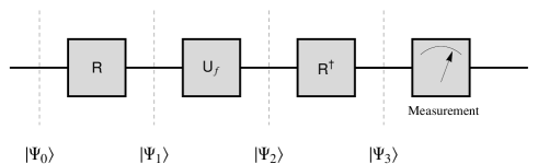
Figure 1: Graphical representation of the operators for the solution of oracle decision problems in continuous variable settings AHS09 .

the Deutsch–Jozsa oracle decision problem employing logical states encoded in the infinite-dimensional Hilbert space of the harmonic oscillator AHS09 ; AHS12 . In this case, $\Psi(x)$ is a square-integrable function of the continuous position $x$.

A key aspect of the approach is the physical accessibility of the harmonic oscillator ground state and the availability of linear and quadratic operators that enable us to prepare the logical input state $\left|\Psi_{0}\right\rangle$. Additionally, the operators $\mathsf{R}$ and $\mathsf{R}^{\dagger}$ identified in Fig. 1 are the easily implementable continuous Fourier transform and its inverse. The oracle information is encoded in the logical state by the unitary operator AHS09

$$\mathsf{U}_{f}=\left(\begin{array}[]{cccc}(-1)^{z_{1}}&0&\cdots&0\\ 0&(-1)^{z_{2}}&\cdots&0\\ \vdots&\vdots&\ddots&\vdots\\ 0&0&\cdots&(-1)^{z_{N}}\\ \end{array}\right),$$ (18)

where the $z_{i}$ are the bits of the unknown string given in oracle decision problem Definition 1.

Mapping this algorithm to the finite-dimensional, continuously-parameterized coherent spin system must first deal with the step that takes the ground state of the spin system to the logical input state $\left|\Psi_{0}\right\rangle$. This first step also employs physically accessible, linear spin rotation and quadratic spin squeezing.

III The Spin System Model

The method of generalized coherent states has been successfully used to describe a number of diverse physical phenomena including quantum optics, atom-light interactions, and superfluidity Pe72 . Here we make use of coherent spin states Ra71 ; Ar72 in creating an alternative model of continuous variable quantum computation. Just as squeezing is beneficial in continuous variable quantum computing using the harmonic oscillator, we make use of spin squeezing here KU93 . We use the optimally squeezed spin state KU93 as input to our algorithm and show that it can be approximated by a superposition of two discrete states with constant error independent of the size of the Hilbert Space.

III.1 Coherent Spin States

Our spin system is a collection of $2S$ elementary $1/2$ spins. $2S$ is an odd integer, and we choose $2S+1=N$ so that $N=2^{n}$-bit strings may be naturally represented. We refer this as an $S$-spin system KU93 .

The system dynamics are determined by the Hamiltonian, which is expressed as a polynomial of su(2) algebraic elements. These algebraic elements are Pauli spin operators in the spin-1/2 single-particle case. For higher even dimensions, we use notation similar to KU93 with operators $\hat{\mathsf{S}}_{i}$, $\hat{\mathsf{S}}_{j}$ and $\hat{\mathsf{S}}_{k}$ and $i,j,k$ denoting the components of any three orthogonal directions, such that

$$\left[\hat{\mathsf{S}}_{i},\hat{\mathsf{S}}_{j}\right] ={\rm{i}}\hat{\mathsf{S}}_{k},$$ (19)

and

$$\Delta\hat{\mathsf{S}}^{2}_{i}\Delta\hat{\mathsf{S}}^{2}_{j} \geq\frac{1}{4}\left\langle\hat{\mathsf{S}}_{k}\right\rangle^{2},$$ (20)

and cyclic permutations.

The spin system is oriented in the usual way. With

$$m\in\left\{-s,-s+1,-s+2,\ldots,s\right\},$$ (21)

the spin kets $\left|m\right\rangle_{s}$ are eigenstates of $\hat{\mathsf{S}}_{z}$ and $\mathsf{S}^{2}$ satisfying

$$\hat{\mathsf{S}}_{z}\left|m\right\rangle_{s} =m\left|m\right\rangle_{s},$$ (22)

and

$$\mathsf{S}^{2}\left|m\right\rangle_{s} =s(s+1)\left|m\right\rangle_{s},$$ (23)

where $\mathsf{S}^{2}=\hat{\mathsf{S}}_{x}^{2}+\hat{\mathsf{S}}_{y}^{2}+\hat{\mathsf{S}}_{z}^{2}$. The ladder operators are $\hat{\mathsf{S}}_{\pm}=\hat{\mathsf{S}}_{x}\pm{\rm i}\hat{\mathsf{S}}_{y}$, and the action of the lowering operator on the ground state is

$$\hat{\mathsf{S}}_{-}\left|-s\right\rangle_{s}=0.$$ (24)

We use the discrete spin states to construct the continuously parameterized coherent spin states.

The harmonic oscillator coherent states are translations of the oscillator ground state Le97 . Analogously, the coherent spin states are rotations of the spin system ground state KU93 ; Ar72 ; Pe72 . Individual spin states are often referred to in the literature Ar72 ; Pe72 as Dicke states analogous to photon number states, and the coherent spin states are referred to as Bloch states analogous to Glauber states.

The coherent spin state, $\left|\theta,\phi\right\rangle_{s}$ with  $\theta,\phi\in\mathbb{R}$, is KU93 :

$$\left|\theta,\phi\right\rangle_{s} =\mathsf{R}_{\theta,\phi}\left|-s\right\rangle_{s}$$

$$=\left(1+\tan^{2}\frac{\theta}{2}\right)^{-s}\times$$

$$\phantom{=}\,\sum_{k=0}^{2s}{2s\choose k}^{\frac{1}{2}}\left(e^{{\rm{i}}\phi}\tan{\frac{\theta}{2}}\right)^{k}\left|s-k\right\rangle_{s}.$$ (25)

The coherent spin state of most interest is

$$\left|\pi/2,0\right\rangle_{s}=2^{-s} \sum_{k=0}^{2s}{2s\choose k}^{\frac{1}{2}}\left|s-k\right\rangle_{s},$$ (26)

which has a Dicke-state amplitude spectrum whose squared magnitude is the binomial probability distribution with $p=q=1/2$ shown in Fig. 2b.

Quasi-probability distributions Pe72 are a useful means of visualizing spin states. We choose to use Q-functions Pe72 as coherent-state representations. The spherical plots of these distributions provide good intuition as to the orientation and the isotropic or anisotropic distribution of uncertainties, but they are not used to actually calculate uncertainties, which is performed using Eq. (20).

For the arbitrary coherent spin state represented as $\left|\Psi\right\rangle=\sum_{k=0}^{2s}\alpha_{k}\left|k\right\rangle$, we express the spherical Q-function Le97 as

$$Q(\theta,\phi)= \sum_{k=0}^{2s}{2s\choose k}^{\frac{1}{2}}\sin(\theta/2)^{k}\cos(\theta/2)^{2s-k}\alpha_{k}e^{{\rm{i}}k\phi}.$$ (27)

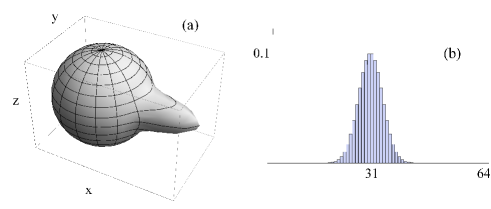
Figure 2: (a) Spherical Q-function of the state given by Eq. (26) for $s=\frac{63}{2}$, and (b) Plot of the respective Dicke-state probability distribution.

In Fig. 2, we plot the spherical Q-function and the probability distribution of the discrete spin state for the state given in Eq. (26). Note that this coherent spin state appears as an ‘equatorial’ state with isotropic uncertainty distribution when represented this way.

III.2 Squeezed Spin States

Coherent spin states can be squeezed KU93 . Whereas the Glauber states can be squeezed to an arbitrary degree, spin states can only be squeezed to the Heisenberg limit of $1/2$ KU93 . We wish to exploit the squeezed state with the minimal achievable variance in our algorithm. In the following, we formulate expressions for this optimally squeezed spin state and show that it can be approximated well by a superposition of two spin states.

We employ two-axis counter-twisting KU93 to define the squeezing operator

$$\mathsf{S}_{\mu}= e^{\rm{i}\frac{\pi}{4}\hat{\mathsf{S}}_{x}}e^{\rm{i}\mu\left(\hat{\mathsf{S}}^{2}_{z}-\hat{\mathsf{S}}^{2}_{y}\right)},$$ (28)

where $\mu$ is the squeezing parameter KU93 . The rotation operator $e^{\rm{i}\frac{\pi}{4}\hat{\mathsf{S}}_{x}}$ orients the resulting anisotropic uncertainty distribution in the $y,z$ directions.

Applying the operator $\mathsf{S}_{\mu}$ to

$$\left|\Psi\right\rangle=\left|\pi/2,0\right\rangle_{s}$$ (29)

allows us to reduce the variance $\Delta\hat{\mathsf{S}}^{2}_{z}$ at the expense of enhancing the variance $\Delta\hat{\mathsf{S}}^{2}_{y}$. The reduced variance may be expressed as

$$V_{-}=\langle\hat{\mathsf{S}}^{2}_{z}\rangle=\left\langle\Psi\right|\mathsf{S}^{\dagger}_{\mu}\hat{\mathsf{S}}^{2}_{z}\mathsf{S}_{\mu}\left|\Psi\right\rangle$$ (30)

since the first moment $\langle\hat{\mathsf{S}}_{z}\rangle=0$. In Fig. 3a, we plot the quasi-probability distribution of a squeezed spin state. The reduced variance of the squeezed state in the $z$ direction and increased variance in the $y$ direction is evident.

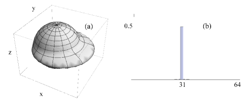
Figure 3: (a) Spherical Q-function of the squeezed state given by Eq. (III.2) for $s=\frac{63}{2}$, and (b) Plot of the respective Dicke-state probability distribution.

The minimum value of the reduced variance $V_{-}$ asymptotically approaches 1/2 with increasing $s$ KU93 . We refer to the optimal value of the squeezing parameter at this minimum as $\mu_{\text{opt}}$. For $\mu>\mu_{\text{opt}}$, the distribution variance increases and the distribution quasi-probability distribution becomes skewed  KU93 . It can shown be that $\mu_{\text{opt}}\rightarrow\frac{1}{s}$ as $s\rightarrow\infty$. This limit is understandable since the variance of a binomial distribution with $p=q=1/2$ is $N/4$, and squeezing simply has the effect of removing the distribution variance of the dependency on $N=2s+1$.

We express the optimally squeezed spin state as

$$\left|\Phi^{(N)}\right\rangle =\left|\pi/2,0,\mu_{\text{opt}}\right\rangle_{s}$$

$$=\mathsf{S}_{\mu_{\text{opt}}}\left|\Psi\right\rangle,$$ (31)

with $\left|\Psi\right\rangle$ defined in Eq. (29). In Fig. 3b, we plot the Dicke-state probability distribution of the optimally squeezed state. It is evident that this state approximates the superposition of two spin states. We wish to provide a bound on how well approximated the squeezed state is by a two-component superposition.

Analysis of the variance of the squeezed state’s probability distribution is facilitated using the qudit representation rather than the spin state representation. We represent this $N$-dimensional squeezed state in terms of the qudits $|i\rangle$ as

$$\left|\Phi^{(N)}\right\rangle=\sum_{i=0}^{N-1}\alpha_{i}|i\rangle.$$ (32)

The probability distribution associated with $\left|\Phi^{(N)}\right\rangle$ may be represented as the set

$$\mathcal{P}^{(N)}=\{\left|\alpha_{0}\right|^{2},\ldots,\left|\alpha_{i}\right|^{2},\ldots,\left|\alpha_{N-1}\right|^{2}\},$$ (33)

with individual probabilities $\mathcal{P}^{(N)}_{i}=\left|\alpha_{i}\right|^{2}$. We note that the squeezed state is symmetric about the centre, and the two central states have

$$\mathcal{P}^{(N)}_{(N/2-1)} =\mathcal{P}^{(N)}_{(N/2)}=P_{c}^{(N)},$$ (34)

and thereby form the principle components of the probability distribution of optimally squeezed states.

For $s>\frac{3}{2}$, the expression for the reduced variance given by Eq. (30) requires solving eigenvalue problems of degree greater than eight and is no longer analytic, and we must resort to numerical analysis. For $s=3/2$ ($N=4$), the expression for the reduced variance given by Eq. (30) is analytic, and $\mu_{\text{opt}}=\frac{\pi}{6\sqrt{3}}$. We represent this optimal squeezed state as

$$\left|\Phi^{(4)}\right\rangle=e^{\rm{i}\phi}\left(0|0\rangle+\frac{1}{\sqrt{2}}|1\rangle+\frac{1}{\sqrt{2}}|2\rangle+0|3\rangle\right),$$ (35)

where $e^{\rm{i}\phi}$ is a global phase picked up by the action of $\mathsf{S}_{\mu}$. The associated probability distribution is

$$\mathcal{P}^{(4)}=\left\{0,1/2,1/2,0\right\}.$$ (36)

For this case we achieve what we refer to as ‘perfect’ squeezing, where ‘perfect’ means that the two central components have probability equal to a half, and the probability of the other two components is zero.

However, this four-component distribution has a variance of only a quarter, where the distribution variance is expressed as

$$\text{Var}\left[\mathcal{P}^{(N)}\right]=\sum_{i=0}^{N-1}i^{2}\left|\alpha_{i}\right|^{2}-\left(\sum_{i=0}^{N-1}i\left|\alpha_{i}\right|^{2}\right)^{2}.$$ (37)

Indeed, for all $N$ if $\mathcal{P}_{c}^{(N)}=1/2$ then,

$$\text{Var}\left[\mathcal{P}^{(N)}\right]= \frac{1}{2}\left((N/2-1)^{2}+(N/2)^{2}\right)-\frac{1}{4}\left(N-1\right)^{2}$$

$$= \frac{1}{4}.$$ (38)

Since the distribution variance approaches 1/2 as $N=2s+1$ approaches infinity, perfect squeezing in the sense we have defined is not possible. We use the variance equals 1/2 as a means to bound $\mathcal{P}_{c}^{(N)}$ defined in Eq. (34). In Fig. 4a,

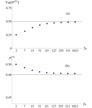
Figure 4: (a) Calculated value of the reduced variance of the probability distribution given by Eq. (30) approaches $1/2$ with increasing $s$ as predicted KU93 . (b) Calculated value of the probability of the two central components given by Eq. (34) is bounded by the constant given by Eq. (41).

we plot the calculated values of the reduced variance given by Eqs. (30) and (37) as a function of $s$ from $s=3/2$ to $s=1023/2$, where we observe that the variance approaches $V=1/2$ as predicted. In order to bound the limiting value of the two central components $\mathcal{P}_{c}^{(N)}$, we bound the ‘tails’ of the probability distribution $\mathcal{P}^{(N)}$.

In Fig. 5, we plot histograms calculated from the squeezed distribution, $\mathcal{P}^{(N)}$, for several values of $s$, where we have scaled the ordinate to reveal the structure of the tail components. We see that the components immediately adjacent to the central components have

$$\mathcal{P}_{N/2+1}^{(N)}=\mathcal{P}_{N/2-2}^{(N)}\approx 0,$$ (39)

and further outlying terms tail off in an exponential-like fashion. We thus introduce the following bounding probability distribution

$$\mathcal{P}_{\mathcal{B}}^{(N)}= \left\{0,\ldots,0,\frac{\epsilon}{3},\frac{2\epsilon}{3},0,\frac{1}{2}-\epsilon,\right.$$ (40)

$$\,\,\,\left.\frac{1}{2}-\epsilon,0,\frac{2\epsilon}{3},\frac{\epsilon}{3},0,\ldots,0\right\},$$

in order to calculate a bound on the two central components of the distribution.

Solving $\text{Var}\left[\mathcal{P}_{\mathcal{B}}^{(N)}\right]=1/2$ for $\epsilon$ gives the probability of the two central components

$$\mathcal{P}_{\mathcal{B}_{c}}^{(N)}=\frac{1}{2}-\epsilon<0.484.$$ (41)

In Fig. 4b, we plot the calculated values of $\mathcal{P}_{c}^{(N)}$, where we note that it goes from 1/2 at $s=3/2$ and asymptotically approaches the constant bounded from below by Eq. (41). The bounding distribution is also overlayed on the histograms presented in Fig. 5.

With these concepts behind us, we state a theorem.

Theorem 1.

The close Hadamard problem, as defined by Problem 1 and Problem 2, can be solved in the spin system model with arbitrarily small error probability in a constant number of oracle queries.

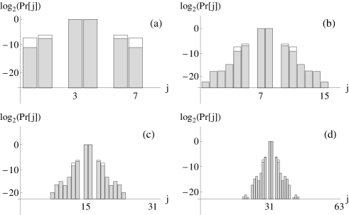
Figure 5: Histograms of the probability distribution $\mathcal{P}^{(N)}$ for (a) $s=7/2$, (b) $s=15/2$, (c) $s=31/2$ and (d) $s=63/2$ with a logarithmic scale for the ordinate. The bounding distribution given by Eqs. (40) and (41) is overlayed on each of the histograms.

Here we briefly recap and summarize the overall approach before proving the theorem in the next section. The spin system model gives us the optimally squeezed state $\left|\Phi^{(N)}\right\rangle$ given by Eq. (32), which forms the input state to the algorithm operators graphically represented in Fig. 1. The input state $\left|\Phi^{(N)}\right\rangle$ has an associated probability distribution $\mathcal{P}^{(N)}$ given by Eq. (33) and bounded by the distribution $\mathcal{P}_{\mathcal{B}}^{(N)}$ given by Eq. (40).

In order to facilitate analysis, we approximate the optimally squeezed state with an idealized input state consisting of the only the two central components. Since greater than $96\%$ of the probability is manifest in the two central components of the bounding distribution as given by Eq. (41), we can replace the optimally squeezed state with the idealized superposition of two states and fold the approximation into the resulting single-query success probability.

This idealized input state can be expressed in a variety of ways. In the qudit representation, it is written

$$\left|\Phi^{(N)}_{\text{\tiny{ideal}}}\right\rangle= 0|0\rangle+...+\frac{1}{\sqrt{2}}|N/2-1\rangle+$$

$$\frac{1}{\sqrt{2}}|N/2\rangle+...+0|N-1\rangle.$$ (42)

In the spin representation with $s=\frac{N-1}{2}$, it is written

$$\left|\Psi^{(s)}_{\text{\tiny{ideal}}}\right\rangle= 0|{-}s\rangle+0|{-s}+1\rangle+...+\frac{1}{\sqrt{2}}|{-}1/2\rangle+$$

$$\frac{1}{\sqrt{2}}|1/2\rangle+...+0|s-1\rangle+0|s\rangle.$$ (43)

Finally in shorthand spin representation, the idealized input state is simply written

$$|\Psi_{0}\rangle=\frac{1}{\sqrt{2}}\left(\left|\frac{1}{2}\right\rangle_{s}+\left|-\frac{1}{2}\right\rangle_{s}\right),$$ (44)

where we have used the subscript zero to represent the algorithm input state in Fig. 1. Proof analysis proceeds by assuming we have a quantum algorithm employing the operators $\mathsf{R}\mathsf{U_{f}}\mathsf{R}^{\dagger}$ given in Fig. 1 with $\mathsf{R}=\mathsf{R}^{\dagger}=\mathsf{H}^{\otimes n}$ acting on the idealized input state given by Eq. (44).

IV Algorithms for the Close Hadamard Problem

In this section we prove Theorem 1 demonstrating what we have an algorithm that solves the close Hadamard problem in the spin system model. We conclude this section with a discussion bounding the performance of classical algorithms in the solution of the close Hadamard problem.

IV.1 Bounding the Performance of the Close Hadamard Algorithm in the Spin System Model

To facilitate analysis in the spin system case, we first use the idealized state given by Eq (44), and then reintroduce the effect of the probability distribution of the optimally squeezed state at the end. We proceed by breaking the proof of Theorem 1 up into two claims one for the restricted case and one for the unrestricted case.

We suppress the normalization factor $\frac{1}{\sqrt{2}}$ and express the idealized input state as

$$\left|\Psi_{0}\right\rangle=\left|\frac{1}{2}\right\rangle_{s}+\left|-\frac{1}{2}\right\rangle_{s}.$$ (45)

We will suppress this normalization factor in all equations having a simple two-component superposition in order to make the equations easier to read. The action of the algorithm on the input state is expressed as

$$\left|\Psi_{3}\right\rangle= \mathsf{H}^{\otimes n}\mathsf{U}_{z}\mathsf{H}^{\otimes n}\left|\Psi_{0}\right\rangle.$$ (46)

The $N$-bit string $z$ represents the function $f$. We show that the algorithm efficiently solves both versions of the close Hadamard problem.

Claim 1.

The restricted close Hadamard problem can be solved with certainty in a single oracle query using the quantum circuit given in Fig. 1 and the idealized input state given by Eq. (45).

Claim 2.

The unrestricted close Hadamard problem can be solved with arbitrarily small error probability in a constant number of oracle queries using the quantum circuit given in Fig. 1 and the idealized input state given by Eq. (45).

A key feature of the input state is that it is a symmetric superposition of two basis states. When Hadamard codewords are encoded into the oracle, the action of the algorithm preserves the symmetric superposition. This preservation is demonstrated in Fig. 6.

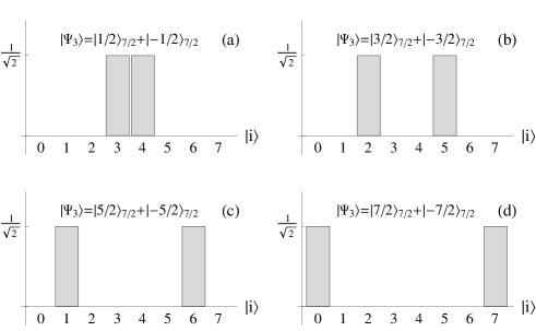
Figure 6: For the example of $s=7/2$, $N=8$, the output state given by Eq. (49) remains a symmetric superposition of two states for the Hadamard codewords: (a) $W^{(8)}_{0}$, (b)$W^{(8)}_{1}$, (c) $W^{(8)}_{2}$, and (d) $W^{(8)}_{3}$.

Lemma 1.

Given the input $\left|\Psi_{0}\right\rangle=\left|\frac{1}{2}\right\rangle_{s}+\left|-\frac{1}{2}\right\rangle_{s}$ to the circuit shown in Fig. 1 and the oracle encoded with one of the Hadamard codewords $z=W_{j}^{(N)}$ for $N=2s+1$ and $0\leq j<\frac{N}{2}$, the output state is another superposition of spin states $\left|\Psi_{3}\right\rangle=\left|\frac{1}{2}+j\right\rangle_{s}+\left|-\frac{1}{2}-j\right\rangle_{s}$.

Proof.

In order to simplify notation in the following, we suppress the superscript $N$ in $W_{j}^{(N)}$. With $W$ defined as the set of Hadamard codewords given by Eq. (2), the pair $(W,\oplus)$ forms a group under addition modulo two Hor07 . In particular, the identity element is $W_{0}$, and each element is its own inverse since

$$W_{j}\oplus W_{j}=W_{0}.$$ (47)

It follows from the group property that the addition of any two codewords is another codeword. For the Hadamard codeword pairs $W_{j}$ and $W_{N-1-j}$, it can be readily shown that

$$W_{j}\oplus W_{N-1-j}=W_{N-1}$$ (48)

for all $j\in\mathbb{Z}_{N}$.

With some algebraic manipulation, the state $\left|\Psi_{3}\right\rangle$ may be expressed as

$$\left|\Psi_{3}\right\rangle= \frac{1}{N}\sum_{y=0}^{N-1}\left(\sum_{x=0}^{N-1}\alpha_{x,y}\right)\left|y\right\rangle.$$ (49)

We use the qudit representation $|y\rangle$ rather than the spin state representation $|m\rangle_{s}$. We translate back to spin state representation as the last step.

The symbol

$$\alpha_{x,y}= (-1)^{\left(z\oplus W_{y+N/2}\right)_{x}}+(-1)^{\left(z\oplus W_{N/2-(y+1)}\right)_{x}},$$ (50)

where $z=W_{j}$ is the string encoded in the oracle, and the symbol $x$ represents the $x^{\rm{th}}$ bit of the $N$-bit strings. Note that the sums $y+N/2$ and $N/2-(y+1)$ in Eq. (50) are modulo $N$ sums.

The Hadamard codewords are balanced with the exception of $W_{0}$, which is constant. For $j\neq k$, this allows us to write

$$0= \sum_{x=0}^{N-1}(-1)^{\left(W_{j}\oplus W_{k}\right)_{x}},$$ (51)

and for $j=k$,

$$N= \sum_{x=0}^{N-1}(-1)^{\left(W_{j}\oplus W_{j}\right)_{x}},$$ (52)

where we have used the group inverse relation given in Eq. (47). Using this result, we see that a non-zero sum of $\alpha_{x,y}$ in Eq. (49) occurs exactly twice when $y=(N/2+j)\mod N$ and when $y=(N/2-1-j)\mod N$.

In the qudit representation, the output state is expressed

$$\left|\Psi_{3}\right\rangle=\left|N/2-1-j\right\rangle+\left|N/2+j\right\rangle,$$ (53)

where qudit indices are understood to be modulo $N$. For $0\leq j<N/2$, this translates back to the spin basis as

$$\left|\Psi_{3}\right\rangle=\left|-1/2-j\right\rangle_{s}+\left|1/2+j\right\rangle_{s},$$ (54)

thus completing the proof of Lemma 1. ∎

We now show that the superposition of two states is also preserved for codewords with restricted errors.

Lemma 2.

Given the input $\left|\Psi_{0}\right\rangle=\left|\frac{1}{2}\right\rangle_{s}+\left|-\frac{1}{2}\right\rangle_{s}$ to the circuit shown in Fig. 1 and the oracle encoded with $z\in\tilde{\Xi}^{(N)}_{j,\,\mathbb{Z}_{N/4}}$ given by Eq. (16), which is a codeword having less than $N/4$ restricted errors, and with $0\leq j<\frac{N}{2}$, the output state is another superposition of spin states $\left|\Psi_{3}\right\rangle=\left|\frac{1}{2}+j\right\rangle_{s}+\left|-\frac{1}{2}-j\right\rangle_{s}$.

Proof.

Observe that the form of Eq. (50) allows for cancelling of errors. Under certain conditions if an error occurs at bit position $x$, the effect on the left-hand side of the plus sign is cancelled by the opposite effect on the right-hand side. Consider the $x^{\rm th}$ bit error in Eq. (50), where we have cancellation

$$0= (-1)^{\left(z\oplus W_{y+N/2}\right)_{x}}+(-1)^{\left(z\oplus W_{N/2-(y+1)}\right)_{x}}.$$ (55)

This identity implies that

$$1 =\left(W_{y+N/2}\oplus W_{N/2-(y+1)}\right)_{x}$$

$$=(W_{N-1})_{x},$$ (56)

where we have used the result expressed in Eq. (48). This is exactly the same as the requirement to be a member of set $\tilde{\Xi}^{(N)}_{j,\,\mathbb{Z}_{N/4}}$ defined in Eq. (16). Under this condition, the result of Lemma 1 holds and $\left|\Psi_{3}\right\rangle=\left|\frac{1}{2}+j\right\rangle_{s}+\left|-\frac{1}{2}-j\right\rangle_{s}$.
∎

We now show that the perfect superposition of two states is no longer preserved for codewords having unrestricted errors. The effect of errors that are not of the restricted type is to degrade the superposition by distributing amplitude evenly across all other states. However, as long as the number of these errors is less than $N/16$, it is still possible to efficiently identify the desired state.

Lemma 3.

Given the input $\left|\Psi_{0}\right\rangle=\left|\frac{1}{2}\right\rangle_{s}+\left|-\frac{1}{2}\right\rangle_{s}$ to the circuit shown in Fig. 1 and the oracle encoded with $z\in\Xi^{(N)}_{j,\,\mathbb{Z}_{N/16}}$ given by Eq. (11), which is a codeword having less than $N/16$ unrestricted errors, the desired state can be identified with success probability of at least $\frac{9}{16}$.

Proof.

Let $V_{j}\in\Xi^{(N)}_{j,1}$ be a Hadamard codeword with a single unrestricted error. We have already shown that if the error is of the restricted type, two-component superpositions are preserved. If the the error is not a restricted error, we have no error cancellation, so the single bit error breaks the balanced and constant sums defined by Eqs. (51) and (52), respectively. For $j\neq k$ this gives

$$2= \sum_{x=0}^{N-1}(-1)^{\left(W_{j}\oplus V_{k}\right)_{x}},$$ (57)

and for $j=k$,

$$N-2= \sum_{x=0}^{N-1}(-1)^{\left(W_{j}\oplus V_{j}\right)_{x}}.$$ (58)

As the input state is a two-component superposition, the above sums result in all the amplitudes of the output state either acquiring or losing an amount of amplitude proportional to four—two from the amount in the balanced or constant sums given in Eqs. (57) and (58) and two from the effect of there being two components in the input state.

We express the output state for the worst case of a single unrestricted error as

$$\left|\Psi_{3}\right\rangle= \frac{1}{\sqrt{2}}\left(1-\frac{4}{N}\right)\left(\left|\frac{1}{2}+j\right\rangle_{s}+\left|-\frac{1}{2}-j\right\rangle_{s}\right)$$

$$+\frac{4}{\sqrt{2}N}\sum_{\stackrel{{\scriptstyle k=-s-1/2}}{{k\neq\pm j}}}^{k=s-1/2}\pm\left|\frac{1}{2}+k\right\rangle_{s}.$$ (59)

For the worst case of $l$ unrestricted errors, where no errors are of the restricted type, the principle components have amplitude

$$\alpha=\frac{1}{\sqrt{2}}\left(1-\frac{4l}{N}\right),$$ (60)

and the amplitude of the next largest component is

$$\beta=\frac{4l}{\sqrt{2}N}.$$ (61)

The amplitude reduction of the principle components by an amount directly proportional to the number of errors results from the constant sum given by Eq. (58) being reduced by double the number of errors. However, the balanced sums are variable since errors can cancel. The worst case occurs when the errors are ‘in phase’ resulting in the amplitude of the next largest component being proportional to the number of errors. The effect of codewords with unrestricted errors on the input superposition is presented in Fig. 7.

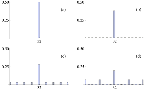
Figure 7: For $N=64$, the effect of $l$ unrestricted errors, where none of the $l$ errors are of the restricted type, on the probability of the central components is demonstrated for (a) $l=0$, (b) $l=2$, (c) $l=4$, and (d) $l=6$. Fig. 7(c) corresponds to the case that $l=N/16$.

The probability of the two central components is

$$\left|\alpha\right|^{2}\geq\frac{1}{2}\left(1-\frac{8l}{N}+\frac{16l^{2}}{N^{2}}\right).$$ (62)

The equality holds for the worst case where none of the errors are of the restricted type. If $l=N/16$, then $\left|\alpha\right|^{2}\geq\frac{1}{2}\left(\frac{9}{16}\right)$. The amplitudes of the two central states can be combined into a single state with amplitude $\sqrt{2}\alpha$ by an appropriate unitary operation. Since $l$ is less than $N/16$, the desired state can be identified with probability $2\left|\alpha\right|^{2}$, which is at least $\frac{9}{16}$. ∎

We use the results of Lemmas 1, 2 and 3 to show that Claims 1 and 2 are true.

Proof of Claim 1:

By Lemmas 1 and 2, $\left|\Psi_{3}\right\rangle=\left|\frac{1}{2}+j\right\rangle_{s}+\left|-\frac{1}{2}-j\right\rangle_{s}$ for $z\in\tilde{\Xi}^{(N)}_{j,\,\mathbb{Z}_{N/4}}$. Immediately prior to the measurement step, we require a unitary operator $\mathsf{U}_{2\mapsto 1}$ that maps this superposition of two states into a single basis state such that

$$\mathsf{U}_{2\mapsto 1}\left|\Psi_{3}\right\rangle=\left|\frac{1}{2}+j\right\rangle_{s}.$$ (63)

Since we know that the unknown string $z$ is either in set $\tilde{\Xi}_{N/2-1}^{(N)}$ or in $\tilde{\Xi}_{k}^{(N)}$, we wish to measure the outcome of the qudit $|s\rangle_{s}$ in the spin basis. We define the projection operator NC00

$$M_{s}=\left|s\right\rangle_{s}\left\langle s\right|,$$ (64)

and outcome probability is

$$\Pr[s]=\left\langle\frac{1}{2}+j\right|_{s}M_{s}\left|\frac{1}{2}+j\right\rangle_{s}.$$ (65)

If $j=N/2-1$, then $\Pr[s]=1$ and $z\in A$, and if $j\neq N/2-1$, then $\Pr[s]=0$ and $z\in B$. Thus, the restricted close Hadamard problem is solved with certainty in a single oracle query. $\square$

Proof of Claim 2:

By Lemmas 1 and 2, $\left|\Psi_{3}\right\rangle=\left|\frac{1}{2}+j\right\rangle_{s}+\left|-\frac{1}{2}-j\right\rangle_{s}$ for $z\in\tilde{\Xi}^{(N)}_{j,\,\mathbb{Z}_{N/4}}$. By Lemma 3, the effect of including $l$ unrestricted bit errors on the output state may be expressed as

$$\left|\Psi_{3}\right\rangle= \alpha\left(\left|\frac{1}{2}+j\right\rangle_{s}+\left|-\frac{1}{2}-j\right\rangle_{s}\right)$$

$$+\beta\sum_{\kappa}\pm\left|\frac{1}{2}+k\right\rangle_{s}+\gamma\sum_{\lambda}\pm\left|\frac{1}{2}+k\right\rangle_{s},$$ (66)

where the symbols $\alpha$ and $\beta$ are given by Eqs. (60) and (61) respectively, and $|\gamma|<|\beta|$. Note that $\kappa+\lambda=N-2$, so that all $N$ possible states are accounted for, but the specific values of $\gamma$, $\kappa$ and $\lambda$ are dependent on $N$ and $l$. The outcome probabilities of measuring the state $|s\rangle_{s}$ are

$$\Pr[s]=\left\langle\frac{1}{2}+j\right|_{s}M_{s}\left|\frac{1}{2}+j\right\rangle_{s}.$$ (67)

If $j=N/2-1$, then $\Pr[s]>\left|\alpha\right|^{2}$, and if $j\neq N/2-1$, then $\Pr[s]<\left|\beta\right|^{2}$. Assuming that the number of unrestricted errors $l$ is less than $N/16$, then an error of $O(e^{-q})$ can be achieved by making $O(q)$ repetitions of the algorithm AHS09 . Thus, the unrestricted close Hadamard problem is solved with arbitrarily small error probability in a constant number of queries. $\square$

Proof of Theorem 1:

In the restricted case, the algorithm output error probability is only due to the error in the input distribution given by Eq. (41). In the unrestricted case, the algorithm output error probability is due to both the error in the input distribution and the inability of the algorithm to accurately distinguish output states when the codeword errors are unrestricted.

For the restricted case, the total success probability is

$$\Pr_{\checkmark}=\mathcal{P}_{c}^{(N)}\Pr[s]_{\text{\tiny{restricted}}}>0.96.$$ (68)

Similarly for unrestricted case, the total success probability is

$$\Pr_{\checkmark}=\mathcal{P}_{c}^{(N)}\Pr[s]_{\text{\tiny{unrestricted}}}>0.54.$$ (69)

Since for each of these cases $\Pr_{\checkmark}>0.5$, then an error of $O(e^{-q})$ can be achieved by making $O(q)$ repetitions of the algorithm AHS09 . This completes the proof of Theorem 1. $\square$

IV.2 Classical Algorithm

In this subsection we compare the performance of any classical algorithm to the performance of the quantum algorithm.

Claim 3.

Any classical deterministic algorithm requires $\Omega(n)$ oracle queries of the bit positions to solve the close Hadamard problem with certainty, even if there are no bit errors. A randomized algorithm with bounded error probability also requires $\Omega(n)$ queries, even if there are no bit errors.

Claim 3 follows from information theoretical considerations. The goal of the classical strategy is to determine which of the $N/2$ Hadamard codewords is loaded into the oracle. The number of possible solutions is then initially $\Omega(2^{n})$. Whenever a classical strategy performs a query, it can eliminate at most half of the remaining possible solutions, even if there are no errors. To reduce the number of possible solutions to a single solution, the classical strategy therefore requires at least $\Omega(n)$ queries. The lower bound also holds when the strings loaded into the oracle are Hadamard codewords with errors.

In the next section we discuss how changing the unitary operators $\mathsf{R}$ and $\mathsf{R}^{\dagger}$ in the algorithm shown in Fig. 1 changes the oracle decision problem that can be solved.

V Alternative Algorithm

The continuously-parameterized, finite-dimensional Hilbert space of the spin system inspired an efficient algorithm for the solution of the close Hadamard problem. The group structure of the Hadamard codewords is implicit in the use of Hadamard operators in the quantum algorithm. We now show that this computation model can inspire other algorithms. Other unitary operators can be employed in the quantum circuit shown in Fig. 1. The discrete Fourier transform NC00 is an obvious alternative. We provide a sketch of how the Fourier transform changes the group structure of the codewords and point to the need for further exploration of problems that could benefit from this computational model.

We replace the operators $\mathsf{R}$ and $\mathsf{R}^{\dagger}$ in Fig. 1 with the discrete Fourier transform $\mathsf{F}$ and $\mathsf{F}^{\dagger}$. The matrix representation of the discrete Fourier transform is expressed as

$$\mathsf{F}^{(N)}=\frac{1}{\sqrt{N}}\left(\begin{array}[]{cccc}1&1&\cdots&1\\ 1&\omega&\cdots&\omega^{N-1}\\ \vdots&\vdots&\ddots&\vdots\\ 1&\omega^{(N-1)}&\cdots&\omega^{(N-1)(N-1)}\\ \end{array}\right),$$ (70)

where $\omega=e^{\frac{\rm{i}\pi}{N}}$ NC00 .

In our analysis of the $\mathsf{F}$-based algorithm, we adopt a similar approach to that taken for the $\mathsf{H}$-based algorithm and define the ‘Fourier codewords’ as

$$\mathsf{T}^{(N)}=\log_{(-1)}\left[\sqrt{N}\mathsf{F}^{(N)}\right].$$ (71)

Similar to the Hadamard codewords, the $j^{\rm th}$ Fourier codeword is the $j^{\rm th}$ row of the matrix $\mathsf{T}^{(N)}$. As an example, we express the $N=8$ matrix as

$$\mathsf{T}^{(8)}=\left(\begin{array}[]{cccccccc}0&0&0&0&0&0&0&0\\ 0&\frac{1}{4}&\frac{1}{2}&\frac{3}{4}&1&-\frac{3}{4}&-\frac{1}{2}&-\frac{1}{4}\\ 0&\frac{1}{2}&1&-\frac{1}{2}&0&\frac{1}{2}&1&-\frac{1}{2}\\ 0&\frac{3}{4}&-\frac{1}{2}&\frac{1}{4}&1&-\frac{1}{4}&\frac{1}{2}&-\frac{3}{4}\\ 0&1&0&1&0&1&0&1\\ 0&-\frac{3}{4}&\frac{1}{2}&-\frac{1}{4}&1&\frac{1}{4}&-\frac{1}{2}&\frac{3}{4}\\ 0&-\frac{1}{2}&1&\frac{1}{2}&0&-\frac{1}{2}&1&\frac{1}{2}\\ 0&-\frac{1}{4}&-\frac{1}{2}&-\frac{3}{4}&1&\frac{3}{4}&\frac{1}{2}&\frac{1}{4}\end{array}\right),$$ (80)

with $T^{(8)}_{4}=01010101$. We see that the Fourier codewords are not bit strings but rather can be thought of as fractional bits. These fractional bits can still be encoded into the oracle function $\mathsf{U}_{z}$ given in Eq. (18).

We define what we term the simple Fourier codeword oracle decision problem and show that it can be solved in a single query using the modified algorithm. Note that we have structured this problem along the same lines as the close Hadamard problem with no errors.

Problem 3.

Given the string $\check{A}=T^{(N)}_{N/2-1}$ and a set of strings $\check{B}=T^{(N)}_{k}$, with $k\in\left\{\mathbb{Z}_{N}\mid k\neq N/2-1\right\}$ and a string $z$ randomly selected with uniform distribution $\mu$ such that $z\in_{\mu}\check{C}=\check{A}\cup\check{B}$, the Simple Fourier Codeword problem is to determine whether $z\in\check{A}$ or $z\in\check{B}$ with the fewest oracle queries.

The action of the algorithm on the input state is expressed as

$$\left|\Psi_{3}\right\rangle= {\mathsf{F}^{{\dagger}}}^{(N)}\mathsf{U}_{z}\mathsf{F}^{(N)}\left(\left|\frac{1}{2}\right\rangle_{s}+\left|-\frac{1}{2}\right\rangle_{s}\right).$$ (81)

For $z=T^{(N)}_{j}$ and $j\in 0,1,\ldots,N-1$, the output state can be shown to be

$$\left|\Psi_{3}\right\rangle= \left|\frac{1}{2}+j\right\rangle_{s}+\left|-\frac{1}{2}+j\right\rangle_{s},$$ (82)

where $\frac{1}{2}+j$ and $-\frac{1}{2}+j$ are modulo $s$ sums in the sense that $\left|\frac{1}{2}+\frac{N}{2}\right\rangle=\left|-s\right\rangle$.

We apply $U_{2\mapsto 1}$ given in Eq. (63) to the state $\left|\Psi_{3}\right\rangle$ given in Eq. (82). Measuring the qudit $|s\rangle_{s}$ in the spin basis with the measurement operator $M_{s}$ given in Eq. (64), distinguishes whether the encoded string is in set $\check{A}$ or set $\check{B}$ thereby solving the simple Fourier codeword problem in a single query.

The result given by Eq. (82) is achieved by exploiting group properties similar to those expressed in Eqs. (47) and (48) for the Hadamard codewords. The columns of $\mathsf{F}^{(N)}$ represent the multiplicative cyclic group of order $N$, where the generator is the first non-trivial column of $\mathsf{F}^{(N)}$. The matrix of codewords $\mathsf{T}^{(N)}$ represents the additive cyclic group of order $N$ as a result of taking the logarithm of $\mathsf{F}^{(N)}$.

Each element of the group has the inverse relation

$$T_{j}+T_{N-j}=T_{0},$$ (83)

and each codeword also obeys the sum relation

$$T_{j}+T_{N/2-j}=T_{N/2},$$ (84)

where $N-j$ and $N/2-j$ are understood to be modulo $N$ sums. In Fig. 8 we clearly see that, unlike, the Hadamard codewords that preserve the superposition of two symmetric states, the Fourier codewords preserve the superposition of two adjacent states.

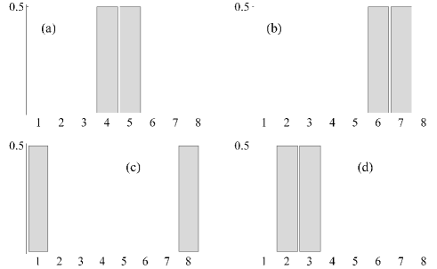
Figure 8: For $s=7/2$, the Fourier-based algorithm probability distributions for the states given by Eq. (82) for (a) $j=0$, (b) $j=2$ (c) $j=4$ and (d) $j=6$. The $\mathsf{F}$-based algorithm preserves the ‘adjacency’ of the input superposition, whereas the $\mathsf{H}$-based algorithm preserves the ‘mirror’ symmetry of the input superposition as shown in Fig. 6.

Comparison of the effect of the different operators is interesting. The Hadamard codewords preserve symmetric superpositions, and there are $N/2$ unique symmetric superpositions. The Fourier codewords preserve adjacent superpositions, and there are $N$ unique adjacent superpositions.

The exploration of the structure of error cancellations along the lines of Eq. (56) using the relationship Eq. (84) for the Fourier codewords may lead to new problems that can be efficiently solved using this model of computation. For example, it is natural to apply this error cancellation concept to the simple Fourier codeword oracle decision problem presented in Problem 3 so that the equivalent of Fourier codewords with errors may be included.

VI Conclusions

We have presented a model of continuous variable quantum computation based on the continuously-parameterized yet finite-dimensional Hilbert space of a spin system. Like continuous variable quantum computation using the states of the harmonic oscillator, this spin system is amenable to physical preparation with linear rotation and quadratic squeezing operators. Unlike the harmonic oscillator case where an arbitrary degree of squeezing may be achieved, spin squeezing occurs in a spherical phase space, and the minimum attainable variance of a spin component asymptotically approaches the Heisenburg limit of one-half KU93 .

We have proposed a pilot oracle decision problem called the close Hadamard problem to demonstrate the type of problem that is amenable to solution using this computational model. We have used a superposition of two discrete states to approximate the optimally squeezed coherent spin state as input into a quantum algorithm presented in Figure 1, which is adapted from the continuously-parameterized infinite-dimensional single mode algorithm AHS09 ; AHS12 .

We have shown that this model of computation solves the close Hadamard problem with arbitrarily small error probability in a constant number of oracle queries. The combination of the model and the algorithm taken together describe a new model of quantum computation. Furthermore, the two versions of the close Hadamard problem hi-light an interesting feature of the model.

The tolerance of errors observed in the restricted case is due to error cancellation, which results from employing the symmetric superposition of spin states as algorithm input combined with the group structure of the Hadamard codewords and the employment of Hadamard operators in the algorithm. This relationship between the structure of the information associated with the problem and the structure of the unitary operators employed in the quantum algorithm is what enables us to solve the restricted problem more efficiently in this computational model. It may prove fruitful to explore the relationship between the error cancellation observed here and how the perturbations related to Grover’s problem mutually cancel in arbitrarily high-dimensional search spaces Jin15 .

We have further explored the relationship between operators and codewords and have shown that it can inspire other algorithms. We have shown that using the discrete Fourier transform as an alternative to the Hadamard operator changes the group structure of the codewords. This in turns indicates that further exploration may lead to the discovery of new problems that would benefit from this computational model. We conclude that the continuously-parameterized representation of quantum dynamical systems having a finite-dimensional Hilbert space gives us a new model of quantum computation that is worthy of further exploration.

References

- (1) Benioff, P., “Quantum mechanical models of Turing machines that dissipate no energy,” Phys. Rev. Lett. 48, pp. 1581–1585 (1982). doi:10.1103/PhysRevLett.48.1581.
- (2) Feynman, R.P., “Simulating physics with computers,” Int. J. Theor. Phys. 21, pp. 467–488 (1982). doi:10.1007/BF02650179.
- (3) Deutsch, D., “Quantum theory, the Church–Turing principle and the universal quantum computer,” Proc. 762 R. Soc. Lond. A 400, pp. 97–117 (1985). doi:10.1098/rspa.1985.0070.
- (4) Adcock, M.R.A., Continuous-Variable Quantum Computation of Oracle Decision Problems, Ph.D. thesis, University of Calgary, (2012). http://theses.ucalgary.ca/bitstream/11023/387/2/ucalgary_2012_adcock_mark.pdf.
- (5) Leonhardt, U., Measuring the Quantum State of Light. Cambridge University Press, Cambridge (1997)
- (6) Deutsch, D., “Quantum computational networks,” Proc. R. Soc. Lond. A, 425, pp. 73–90 (1989). doi:10.1098/rspa.1989.0099.
- (7) Nielsen, M. A., “Cluster-state quantum computation,” Rep. Math. Phys., 57, pp. 147–161 (2006). doi:10.1016/S0034-4877(06)80014-5.
- (8) Perelomov, A., Generalized Coherent States and Their Applications, Springer, New York, (1972).
- (9) Arrechi, F. T., Courtens, E., Gilmore, R., and Thomas, H., “Atomic coherent states in quantum optics,” Phys. Rev. A, 6, pp. 2211–2237, (1972). doi:10.1103/PhysRevA.6.2211.
- (10) Radcliffe, J. M., “Some properties of coherent spin states,” J. Phys. A Gen. Phys., 4, pp. 313 (1971). doi:10.1088/0305-4470/4/3/009.
- (11) Kitagawa, M. and Ueda, M., “Squeezed spin states,” Phys. Rev. A, 47, pp. 5138–5143 (1993). doi:10.1103/PhysRevA.47.5138.
- (12) Adcock, M. R. A., Høyer, P., and Sanders, B. C., “Limitations on continuous variable quantum algorithms with Fourier transforms,” New J. Phys., 11, pp. 103035 (2009). doi:10.1088/1367-2630/11/10/103035.
- (13) Adcock, M. R. A., Høyer, P., and Sanders, B. C., “Gaussian quantum computation with oracle-decision problems,” Quantum Inf. Process., 12, pp. 759 -1779 (2012). doi:10.1007/s11128-012-0489-1.
- (14) MacWilliams, F. J. and Sloane, N. J. A., The Theory of Error-Correcting Codes, North Holland, New York (1977)
- (15) Horadam, K. J., Hadamard Matrices and Their Applications, Princeton University Press, Princeton (2007)
- (16) Bernstein, E. and Vazirani, U., “Quantum Complexity Theory,” In: Proceedings of the Twenty-fifth Annual Association for Computing Machinery Symposium on Theory of Computing, pp. 11–20 (1993). doi:10.1145/167088.167097.
- (17) Mosca, M., Quantum Computer Algorithms, Ph.D. thesis, University of Oxford, (1999). http://www.iqc.ca/~mmosca/web/papers/moscathesis.pdf.
- (18) Deutsch, D. and Jozsa, R., “Rapid solution of problems by quantum computation,” Proc. R. Soc. Lond. A, 439, pp. 553–558 (1992). doi:10.1098/rspa.1992.0167.
- (19) Braunstein, S. L. and Pati, A. K., editors, Quantum Information with Continuous Variables, Kluwer, Dordrecht, (2003)
- (20) Hall, M., “Semi-automorphisms of Hadamard matrices,” Math. Proc. Camb. Philos. Soc, 77, pp. 459–473 (1975). doi:10.1017/S0305004100051288.
- (21) Michelson, A. M. and Levesque, A. H., Error Control Techniques for Digital Communication, Wiley, New York (1985).
- (22) Nielsen, M. A. and Chuang, I. L., Quantum Computation and Quantum Information, Cambridge University Press, Cambridge, (2000)
- (23) Atallah, M. J., Algorithms and Theory of Computation Handbook, CRC Press LLC, Boca Raton, (1998)
- (24) Jin, W. L., “Dynamical Analysis of Grover’s Search Algorithm in Arbitrarily High-Dimensional Search Spaces,” (2015). http://vixra.org/abs/1506.0069