Two quantum walkers sharing coins

Abstract

We consider two independent quantum walks on separate lines augmented by partial or full swapping of coins after each step. For classical random walks, swapping or not swapping coins makes little difference to the random walk characteristics, but we show that quantum walks with partial swapping of coins have complicated yet elegant inter-walker correlations. Specifically we study the joint position distribution of the reduced two-walker state after tracing out the coins and analyze total, classical and quantum correlations in terms of mutual information, quantum mutual information, and measurement-induced disturbance. Our analysis shows intriguing quantum features without classical analogues.

I Introduction

Quantum walks (QWs) ADZ93 are especially interesting because of their importance in quantum algorithms research AAKV01 ; Ken06 and also because they represent an intriguing quantum version of the ubiquitous classical phenomenon of random walks (RWs). Originally conceived as a single walker whose left or right step on a line is entangled with the outcome of flipping a single two-sided quantum coin, the QW has been extended to more general cases of higher-dimensional walks MBSS02 ; FGB11 ; FGMB11 , multiple walkers and/or multiple coins BCA03 ; BCAprl ; SBKKJ11 ; RSSJS11 ; AVWW11 ; AAM+11 ; BW11 . These generalizations enable exploration of QWs in complex settings, which could connect with real-world phenomena such as transport in photosynthetic protein complexes MRLG08 . Additionally the inclusion of more walkers and/or coins can efficiently enlarge the Hilbert space being explored because a linear increase in degrees of freedom exponentially enlarges the Hilbert space.

Here we explore the complex case of two walkers each carrying and (quantumly) flipping separate coins but with the freedom to swap partially the coins between flips. By partial swapping we mean that the two walkers can effect the unitary operation SWAP^τ on their coins: for $\tau=0$, this corresponds to no swapping whatsoever so the two walkers evolve completely independently, and the other extreme is $\tau=1$ corresponding to completely swapping the coins after every step. For $\tau>0$ a consequence of full or partial swapping is to cause entanglement between the walkers’ position and coin degrees of freedom. Classically swapping coins does not change the walker dynamics because each coin flip is random, but quantumly the effect of swapping is important because of the unitary dynamics.

Partial or full swapping of coins is interesting as this simple procedure turns independent QWs into entangled QWs. As multi-walker QWs could occur in nature, our work suggests new phenomena to explore in QW behavior. Although we focus on the two-walker case, the multiple-walker case can be obtained by a natural extension of our foundational work on this area. Full and partial swapping of coins between independent QWers is also appealing practically as an implementation. Each independent walker’s can correspond to the phase of a cavity field, and each walker’s two-sided coin is an atom in the cavity with a superposition of ground and excited electronic energy states coupled to the cavity via a dispersive nonlinear phase shift TM02 ; XS08 ; XSBL08 . The atoms can interact via a dipole-dipole interaction HM09 ; DRKB02 between (or during) steps, and the strength of this dipole-dipole interaction determines the value of $\tau$.

Two-walker QWs are compared to two-walker RWs by examining the joint position distributions of the two walkers after tracing out the coin states. Classically, for any value of $\tau$, no correlation is expected and the diffusion of position is marked by its spread $\sigma$ (standard deviation of the position distribution) increasing as $\sqrt{t}$ for $t$ the elapsed time (which can be expressed as a continuous or a discrete quantity and is the discrete number of steps in our study). Quantum walks can be distinguished by ballistic spreading, where the $\sigma$ grows linearly with $t$ Kem03 or by Anderson-type localization where the walker’s spread becomes constant at large $t$ KLMW07 ; SCP+11 . This localization effect is due to the walker effectively becoming trapped due to irregularities of the spacing of the lattice traversed by the walker. Thus, there are three domains of spreading in the asymptotic large $t$ limit: ballistic ($\sigma\propto t$), diffusive ($\sigma\propto\sqrt{t}$) and localized ($\sigma\sim$constant).

Here we are interested not only in how the walker’s position spreads but also in the correlations between two walkers’ positions after tracing out the coins. To study the correlations, we go beyond evaluating joint position distributions for different values of $t$ to studying two-time correlation functions. Such correlation functions prove to be quite useful for studying two-walker dynamics with partial coin swapping.

II Methods

II.1 One walker

For a single-walker QW on a line, the Hilbert space is

$$\mathscr{H}=\mathscr{H}_{\text{w}}\otimes\mathscr{H}_{\text{c}}$$ (1)

with the walker Hilbert space $\mathscr{H}_{\text{w}}$ spanned by the orthogonal lattice position vectors $\{\left|{x}\right\rangle\}$ and $\mathscr{H}_{\text{c}}$ the two-dimensional coin space spanned by two orthogonal vectors which we denote $\left|{\pm 1}\right\rangle$. Each step by the walker is effected by two subsequent unitary operators: the coin-flip operator

$$C=H=\frac{1}{\sqrt{2}}\begin{pmatrix}1&1\\ 1&-1\end{pmatrix},$$ (2)

for $H$ the Hadamard matrix and the conditional-translation operator

$$S= \sum_{x}\left|{x+1}\right\rangle\left\langle{x}\right|\otimes\left|{1}\right\rangle\left\langle{1}\right|$$

$$+\sum_{x}\left|{x-1}\right\rangle\left\langle{x}\right|\otimes\left|{-1}\right\rangle\left\langle{-1}\right|.$$ (3)

The resultant step operator is $U=S(\mathds{1}\otimes C)$ with $\mathds{1}$ the identity operator on $\mathscr{H}_{\text{w}}$.

The choice of initial state $\big{|}\psi(t=0)\big{\rangle}$ is important in studies of QWs because the interference features sensitively depend on the choice of state. This sensitivity is persistent because the dynamics are unitary hence do not die out. On the other hand the general properties of QWs do not depend on the choice of initial state so the choice of initial state is not crucial provided that the focus is on such characterization.

As we are interested in general properties, the initial state is not important so we choose the initial product state with the walker at the origin of the two-dimensional lattice and hold separate coins in an equal superposition of the $+1$ and $-1$ states:

$$\big{|}\psi(t=0)\big{\rangle}=\frac{1}{\sqrt{2}}\left|{0}\right\rangle(\left|{1}\right\rangle+i\left|{-1}\right\rangle).$$ (4)

The differences between QWs and RWs are due to interference effects (or entanglement) between coin and walkers after several applications of $U$ (with the number of applications $t$ being the discrete time variable). We perform a measurement at some point in order to know the outcome of the walk. The measurement of the walker’s position corresponds to the projection-valued measure $\big{\{}\left|{x}\right\rangle\left\langle{x}\right|;x\in\mathbb{Z}\big{\}}$ resulting in the walker’s state ‘collapsing’ to position $x$ on the lattice. After $t$ steps, the final state of the system is $\left|{\psi(t)}\right\rangle=U^{t}\left|{\psi(0)}\right\rangle$. The reduced state of the walker is obtained by tracing out the coin.

The probability $P(x;t)$ that the walker will be found at the position $x$ is

$$P(x;t)=\left\langle{x}\right|\text{Tr}_{\text{c}}\left(\left|{\psi(t)}\right\rangle\left\langle{\psi(t)}\right|\right)\left|{x}\right\rangle,$$ (5)

which is obtained by tracing out the coin of the walker-coin state and then measuring the walker’s position. We can characterize $P(x;t)$ by the moments of this position distribution $\langle x^{m}\rangle$. The mean $\langle x\rangle$ and variance $\langle x^{2}\rangle-\langle x\rangle^{2}$ can be used as the measure of QWs and show the signature of QWs compared to RWs. For a RW, the position variance $\sim t$, which is characteristic of diffusive motion, whereas, for a QW, a quadratic enhancement is achieved: the position variance $\sim t^{2}$ Kem03 .

II.2 Two walkers

The extension to two independent quantum walkers is straightforward. The new Hilbert space is $\mathscr{H}\otimes\mathscr{H}$, and the step operator is $U\otimes U$. The walkers evolve independently of each other. To entangle the walkers and their respective coins together, we change the step operator from $U\otimes U$ to $\text{SWAP}^{\tau}(U\otimes U)$ for

$$\text{SWAP}^{\tau}=\frac{1}{2}\begin{pmatrix}2&0&0&0\\ 0&1+(-1)^{\tau}&1-(-1)^{\tau}&0\\ 0&1-(-1)^{\tau}&1+(-1)^{\tau}&0\\ 0&0&0&2\\ \end{pmatrix}$$ (6)

expressed in the basis that naturally extends from the single-walker case via the tensor product of Hilbert spaces.

The full initial state of the two-walker system is $\left|{\psi(0)}\right\rangle\otimes\left|{\psi(0)}\right\rangle$ (each walker is initially localized at the origin of their respective lines). After $t$ steps, the final state of the two-walker+coins system is

$$\left|{\psi(t)}\right\rangle_{12}=U_{2}^{t}\left|{\psi(0)}\right\rangle_{1}\otimes\left|{\psi(0)}\right\rangle_{2}$$ (7)

with $U_{2}=\text{SWAP}^{\tau}(U\otimes U)$. We now follow the evolution by performing a Fourier transform of the evolution operator to the “momentum” $k$ space.

The eigenvectors

$$\left|{k}\right\rangle=\sum_{x}e^{ikx}\left|{x}\right\rangle,$$ (8)

of $S$ and $S^{\dagger}$ in Eq. (II.1) have the eigenrelations

$$S\left|{k}\right\rangle=e^{-ik}\left|{k}\right\rangle,S^{\dagger}\left|{k}\right\rangle=e^{ik}\left|{k}\right\rangle$$ (9)

for $k$ a continuous real quantity. The inverse transformation is

$$\left|{x}\right\rangle=\int^{\pi}_{-\pi}\frac{\text{d}k}{2\pi}e^{-ikx}\left|{k}\right\rangle.$$ (10)

Each walker is initialized at the origin of the line so each walker’s initial state is

$$\left|{0}\right\rangle=\int^{\pi}_{-\pi}\frac{\text{d}k}{2\pi}\left|{k}\right\rangle.$$ (11)

In the $\{\left|{k}\right\rangle\}$ and $\{\left|{j}\right\rangle\}$ bases for the two wakers, where $j$ is a continuous index for the momentum of the second walker, the evolution operator becomes

$$U_{2}\left|{k}\right\rangle\otimes\left|{j}\right\rangle\otimes\left|{\Phi}\right\rangle_{\text{c}}=\left|{k}\right\rangle\otimes\left|{j}\right\rangle\otimes U_{kj}\left|{\Phi}\right\rangle_{\text{c}},$$ (12)

with $\left|{\Phi}\right\rangle_{\text{c}}$ the coin state and

$$U_{kj}=\text{SWAP}^{\tau}U_{k}\otimes U_{j},$$ (13)

where

$$U_{k(j)}=\begin{pmatrix}e^{-ik(j)}&e^{-ik(j)}\\ e^{ik(j)}&-e^{ik(j)}\\ \end{pmatrix}.$$ (14)

The $k$ and $j$ subscripts are of course the continuous walker-momentum eigenvalues.

The general density operator for the initial state of the system in the $k$ basis can be expressed as

$$\rho(0)=\int_{-\pi}^{\pi}\frac{\text{d}k}{2\pi}\int_{-\pi}^{\pi}\frac{\text{d}k^{\prime}}{2\pi}\int_{-\pi}^{\pi}\frac{\text{d}j}{2\pi}\int_{-\pi}^{\pi}\frac{\text{d}j^{\prime}}{2\pi}\left|{k}\right\rangle\left\langle{k^{\prime}}\right|\otimes\left|{j}\right\rangle\left\langle{j^{\prime}}\right|\otimes\left|{\Phi_{0}}\right\rangle\left\langle{\Phi_{0}}\right|.$$ (15)

The final state after $t$ steps is

$$\rho(t)=\frac{1}{(2\pi)^{4}}\int_{-\pi}^{\pi}\text{d}k\int_{-\pi}^{\pi}\text{d}k^{\prime}\int_{-\pi}^{\pi}\text{d}j\int_{-\pi}^{\pi}\text{d}j^{\prime}\left|{k}\right\rangle\left\langle{k^{\prime}}\right|\otimes\left|{j}\right\rangle\left\langle{j^{\prime}}\right|\otimes U_{kj}^{t}\left|{\Phi_{0}}\right\rangle\left\langle{\Phi_{0}}\right|(U_{kj}^{\dagger})^{t}.$$ (16)

In terms of the superoperator $\mathcal{L}_{kk^{\prime}jj^{\prime}}\hat{O}=U_{kj}\hat{O}U_{kj}^{\dagger}$,

$$\rho(t)=\frac{1}{(2\pi)^{4}}\int_{-\pi}^{\pi}\text{d}k\int_{-\pi}^{\pi}\text{d}k^{\prime}\int_{-\pi}^{\pi}\text{d}j\int_{-\pi}^{\pi}\text{d}j^{\prime}\left|{k}\right\rangle\left\langle{k^{\prime}}\right|\otimes\left|{j}\right\rangle\left\langle{j^{\prime}}\right|\otimes\mathcal{L}^{t}_{kk^{\prime}jj^{\prime}}\left|{\Phi_{0}}\right\rangle\left\langle{\Phi_{0}}\right|.$$ (17)

The walkers’ positions are on a two-dimensional integer lattice labeled $(x,y)$ with the initial position localized at $(0,0)$. Measurement of the first walker’s position corresponds to the projection-valued measure $\{|x\rangle\langle x|\otimes\mathds{1};x\in\mathbb{Z}\}$ on the two-walker reduced state (after tracing out the coins), and the second walker’s position measurement is $\{\mathds{1}\otimes|y\rangle\langle y|;y\in\mathbb{Z}\}$. Joint measurement of the two walkers’ positions corresponds to the projection-valued measure

$$\{|x\rangle\langle x|\otimes|y\rangle\langle y|;(x,y)\in\mathbb{Z}^{2}\}$$

acting on the reduced two-walker state.

The joint position distribution $P(x,y;t)$ of finding the first walker at $x$ and the second at $y$ is

$$P(x,y;t)=\!_{1}\left\langle{x}\right|_{2}\left\langle{y}\right|\rho_{\text{w}}(t)\left|{y}\right\rangle_{2}\left|{x}\right\rangle_{1},$$ (18)

at time $t$ where

$$\rho_{\text{w}}(t)=\text{Tr}_{\text{c}}(\left|{\psi(t)}\right\rangle_{12}\left\langle{\psi(t)}\right|)$$ (19)

is the state of the two walkers obtained by tracing out the coins. Thus the position distribution of each walker at position $x$ (the case for $y$ is similar) is obtained by tracing out the states of the two coins and the other walker

$$P_{1}\left(x;t\right)=\left\langle{x}\right|\text{Tr}_{2}\rho_{\text{w}}(t)\left|{x}\right\rangle,$$

$$P_{2}\left(y;t\right)=\left\langle{y}\right|\text{Tr}_{1}\rho_{\text{w}}(t)\left|{y}\right\rangle.$$ (20)

The variance of the position distribution is especially important. For standard QWs with single walkers, the variance of the position distribution has been shown to evolve according to $\sigma\propto t^{2}$, whereas $\sigma\propto t$ for RWs. This quadratic speedup of spreading in a unitary evolution is a hallmark of the QW on a line. For our case, namely QWs with two walkers switching their coin partially for each step, the variance of each walker distribution can still be used to qualify the quantum behavior of this kind walks.

If we trace out the second walker, the reduced density matrix is

$$\rho_{1}(t) =\sum_{y}\text{Tr}\left\{\left|{y}\right\rangle\left\langle{y}\right|\rho(t)\right\}$$

$$=\frac{1}{(2\pi)^{4}}\int_{-\pi}^{\pi}\text{d}k\int_{-\pi}^{\pi}\text{d}k^{\prime}\int_{-\pi}^{\pi}\text{d}j\int_{-\pi}^{\pi}\text{d}j^{\prime}\left|{k}\right\rangle\left\langle{k^{\prime}}\right|\sum_{y}e^{-i(j-j^{\prime})y}\text{Tr}\left(\mathcal{L}^{t}_{kk^{\prime}jj^{\prime}}\left|{\Phi_{0}}\right\rangle\left\langle{\Phi_{0}}\right|\right).$$ (21)

The sum can be exactly carried out in terms of derivatives of the $\delta$ function:

$$\frac{1}{2\pi}\sum_{y}y^{m}e^{-(j-j^{\prime})y}=(-i)^{m}\delta^{(m)}(j-j^{\prime}).$$ (22)

Inserting this result back into the expression of the reduced density matrix yields

$$\rho_{1}(t)=\frac{1}{(2\pi)^{3}}\int_{-\pi}^{\pi}\text{d}k\int_{-\pi}^{\pi}\text{d}k^{\prime}\int_{-\pi}^{\pi}\text{d}j\left|{k}\right\rangle\left\langle{k^{\prime}}\right|\text{Tr}\left(\mathcal{L}^{t}_{kk^{\prime}j}\left|{\Phi_{0}}\right\rangle\left\langle{\Phi_{0}}\right|\right).$$ (23)

The probability for the first walker to reach a point $x$ at time $t$ is

$$P_{1}(x;t) =\text{Tr}\left\{\left|{x}\right\rangle\left\langle{x}\right|\rho_{1}(t)\right\}$$

$$=\frac{1}{(2\pi)^{3}}\int_{-\pi}^{\pi}\text{d}k\int_{-\pi}^{\pi}\text{d}k^{\prime}\int_{-\pi}^{\pi}\text{d}je^{-i(k-k^{\prime})x}\text{Tr}\left(\mathcal{L}^{t}_{kk^{\prime}j}\left|{\Phi_{0}}\right\rangle\left\langle{\Phi_{0}}\right|\right).$$ (24)

Thus we can calculate the moments of this distribution:

$$\langle x^{m}\rangle_{t} =\sum_{x}x^{m}P(x;t)$$

$$\frac{(-1)^{m}}{(2\pi)^{3}}\int_{-\pi}^{\pi}\text{d}k\int_{-\pi}^{\pi}\text{d}k^{\prime}\int_{-\pi}^{\pi}\text{d}j\delta^{(m)}(k-k^{\prime})\text{Tr}\left(\mathcal{L}^{t}_{kk^{\prime}j}\left|{\Phi_{0}}\right\rangle\left\langle{\Phi_{0}}\right|\right).$$ (25)

For the first moment, we obtain

$$\langle x\rangle_{t} =\frac{-i}{(2\pi)^{2}}\int_{-\pi}^{\pi}\text{d}k\int_{-\pi}^{\pi}\text{d}j\frac{\text{d}}{\text{d}k}\text{Tr}\left(\mathcal{L}^{t}_{kj}\left|{\Phi_{0}}\right\rangle\left\langle{\Phi_{0}}\right|\right)$$

$$=-\frac{1}{(2\pi)^{2}}\int_{-\pi}^{\pi}\text{d}k\int_{-\pi}^{\pi}\text{d}j\sum_{l=1}^{t}\text{Tr}\left(Z_{1}\mathcal{L}^{l}_{kj}\left|{\Phi_{0}}\right\rangle\left\langle{\Phi_{0}}\right|\right),$$ (26)

where $Z_{1}=\sigma_{z}\otimes\mathds{1}$. We can carry out a similar integration by parts to obtain the second moment:

$$\langle x^{2}\rangle_{t}=\frac{1}{(2\pi)^{2}}\int_{-\pi}^{\pi}\text{d}k\int_{-\pi}^{\pi}\text{d}j\left\{\sum_{l=1}^{t}\sum_{l^{\prime}=1}^{l}\text{Tr}\left[Z_{1}\mathcal{L}^{l-l^{\prime}}_{kj}\left(Z_{1}\mathcal{L}_{kj}^{l^{\prime}}\left|{\Phi_{0}}\right\rangle\left\langle{\Phi_{0}}\right|\right)\right]+\sum_{l=1}^{t}\sum_{l^{\prime}=1}^{l-1}\text{Tr}\left[Z_{1}\mathcal{L}^{l-l^{\prime}}_{kj}\left(\left(\mathcal{L}_{kj}^{l^{\prime}}\left|{\Phi_{0}}\right\rangle\left\langle{\Phi_{0}}\right|\right)Z_{1}\right)\right]\right\}.$$ (27)

For $\tau=0$, the two-walker QW turns to be the standard Hadamard walk for each walker. The first and second moments of the distribution behave as same as those for the standard Hadamard walk. That is, $\langle x\rangle_{t}$ is linear dependent on $t$, while $\langle x^{2}\rangle_{t}$ is quadratic dependent on $t$.

For $0<\tau\leq 1$, $U_{kj}$ is still unitary. For short time, the moments of the position distribution behave similarly to those for standard unitary walk. In the long-time limit we can solve the moments of distribution analytically. Suppose $\mathcal{L}_{kj}$ is a linear transformation and all the eigenvalues satisfy $|\lambda|\leq 1$. We drop the terms that will be zero at large $t$ from the expressions for the moments.

As $\mathcal{L}_{kj}$ is linear, we can represent it as a matrix acting on the space of $4\times 4$ operators. We choose the representation to be

$$\hat{O}=r_{1}\mathds{1}^{12}+r_{2}\mathds{1}^{1}\otimes\sigma^{2}_{x}+\cdot\cdot\cdot+r_{16}\sigma_{z}^{1}\otimes\sigma_{z}^{2}.$$ (28)

The action of $\mathcal{L}_{kj}$ on $\hat{O}$ is given by the matrix

$$\mathcal{L}_{kj}\hat{O}=M_{kj}(r_{1}\;r_{2}\cdots\;r_{16})$$ (29)

with none-zero matrix elements

$$(M_{kj})_{1,1}=(M_{kj})_{4,4}=(M_{kj})_{13,13}=(M_{kj})_{16,16}=\frac{1}{4}\left[-(1+e^{i\pi\tau})\cos(k-j)+2\cos(k+j)\right],$$

$$(M_{kj})_{1,4}=(M_{kj})_{4,1}=(M_{kj})_{13,16}=(M_{kj})_{16,13}=\frac{1}{8}e^{-i(k+j)}\left\{2+\left[1+(-1)^{\tau}\right]e^{2ij}-\left[1+(-1)^{\tau}+2e^{2ij}\right]e^{2ik}\right\},$$

$$(M_{kj})_{1,13}=(M_{kj})_{4,16}=(M_{kj})_{13,1}=(M_{kj})_{16,4}=\frac{1}{8}e^{-i(k+j)}\left\{2-\left[1+(-1)^{\tau}\right]e^{2ij}+\left[1+(-1)^{\tau}-2e^{2ij}\right]e^{2ik}\right\},$$

$$(M_{kj})_{1,16}=(M_{kj})_{4,13}=(M_{kj})_{13,4}=(M_{kj})_{16,1}=\frac{1}{4}\left[(1+e^{i\pi\tau})\cos(k-j)+2\cos(k+j)\right],$$

$$(M_{kj})_{6,6}=i(M_{kj})_{6,7}=-i(M_{kj})_{7,6}=(M_{kj})_{7,7}=i(M_{kj})_{10,6}=-(M_{kj})_{10,7}=(M_{kj})_{11,6}=i(M_{kj})_{11,7}$$

$$=-\frac{1}{4}\left[-1+(-1)^{\tau}\right]e^{i(j-k)},$$

$$(M_{kj})_{6,10}=i(M_{kj})_{6,11}=i(M_{kj})_{7,10}=-(M_{kj})_{7,11}=-i(M_{kj})_{10,10}=(M_{kj})_{10,11}=(M_{kj})_{11,10}=i(M_{kj})_{11,11}$$

$$=i\frac{1}{4}\left[-1+(-1)^{\tau}\right]e^{i(j-k)}.$$ (30)

In the integrand, the initial density matrix for the coins is multiplied $l$ times by $\mathcal{L}_{kj}$ then multiplied on the left by $Z_{1}$ and finally the trace is taken. As $\text{Tr}\left\{\hat{O}\right\}=r_{1}+r_{4}+r_{13}+r_{16}$, $\langle x\rangle_{t}$ is the same as multiplying the vector $(r_{1}\;r_{2}\;\cdots r_{16})^{T}$ $l$ times by $M_{kj}$ and then keeping only the $r_{1}$, $r_{4}$,$r_{13}$ and $r_{16}$ components of the result. This gives the new expression of the first moment as

$$\langle x\rangle_{t} =-\frac{1}{(2\pi)^{2}}\int_{-\pi}^{\pi}\text{d}k\int_{-\pi}^{\pi}\text{d}j\left(1\;0\;0\;1\;0\;\cdots\;0\;1\;0\;0\;1\right)\sum_{l=1}^{t}M_{kj}^{l}(r_{1}\;r_{2}\;\cdots\;r_{16})^{T}$$

$$=-\frac{1}{(2\pi)^{2}}\int_{-\pi}^{\pi}\text{d}k\int_{-\pi}^{\pi}\text{d}j\sum_{l}^{t}\left(M_{kj}^{l}-2\left|{1}\right\rangle\left\langle{1}\right|\otimes\mathds{1}M_{kj}^{l}\right)(r_{1}\;r_{2}\;\cdots\;r_{16})^{T},$$ (31)

which is independent on $t$ in the long time limit since $M_{kj}^{t}\rightarrow 0$ with all the eigenvalues of $M_{kj}$ satisfying $0<|\lambda|\leq 1$. We then obtain

$$\langle x\rangle_{t}\approx\left\{1-\frac{2}{(2\pi)^{2}}\int_{-\pi}^{\pi}\text{d}k\int_{-\pi}^{\pi}\text{d}j\text{Tr}\left[\left|{1}\right\rangle\left\langle{1}\right|\otimes\mathds{1}(1-\mathcal{L}_{kj})^{-1}\mathcal{L}_{kj}\left|{\Phi_{0}}\right\rangle\left\langle{\Phi_{0}}\right|\right]\right\}t+\text{oscillatory terms}.$$ (32)

For the second moment of the distribution, the superoperator $\mathcal{L}_{kj}$ is unitary and preserves the identity, $\mathcal{L}_{kj}\mathds{1}=\mathds{1}$. We will separate the traceless part $\chi_{0}$ of the coins’ initial state from the overall state BCA03 ; BCAprl ,

$$r_{1}\mathds{1}+(\left|{\Phi_{0}}\right\rangle\left\langle{\Phi_{0}}\right|-r_{1}\mathds{1})\equiv r_{1}\mathds{1}+\chi_{0}.$$ (33)

then insert this result into the expression for the second moment of the distribution to obtain

$$\langle x^{2}\rangle_{t}= \frac{1}{(2\pi)^{2}}\int_{-\pi}^{\pi}\text{d}k\int_{-\pi}^{\pi}\text{d}j\Big{\{}\text{Tr}\left[\sum_{l=1}^{t}\mathcal{L}_{kj}^{l}(r_{1}\mathds{1}+\chi_{0})\right]+2r_{1}\text{Tr}\left[Z_{1}\sum_{l=1}^{t}\sum_{l^{\prime}=1}^{l-1}\mathcal{L}_{kj}^{(l-l^{\prime})}Z_{1}\right]$$

$$+\sum_{l=1}^{t}\sum_{l^{\prime}=1}^{l-1}\text{Tr}\left[Z_{1}\mathcal{L}^{l-l^{\prime}}_{kj}\left(Z_{1}(\mathcal{L}^{l}_{kj}\chi_{0})+(\mathcal{L}^{l}_{kj}\chi_{0})Z_{1}\right)\right]\Big{\}}\approx C_{2}t^{2}+\text{const.}+\text{oscillatory terms},$$ (34)

where

$$C_{2}=1+\frac{1}{(2\pi)^{2}}\int_{-\pi}^{\pi}\text{d}k\int_{-\pi}^{\pi}\text{d}j\text{Tr}\left[-2Z_{1}\left(1-\mathcal{L}_{kj}\right)^{-1}\mathcal{L}_{kj}\left|{\Phi_{0}}\right\rangle\left\langle{\Phi_{0}}\right|\left|{1}\right\rangle\left\langle{1}\right|\otimes\mathds{1}-4\left|{1}\right\rangle\left\langle{1}\right|\otimes\mathds{1}\left(1-\mathcal{L}_{kj}\right)^{-1}\mathcal{L}_{kj}\left|{\Phi_{0}}\right\rangle\left\langle{\Phi_{0}}\right|\right].$$ (35)

In brief the first and second moments of the position distribution are linearly and quadratically dependent on $t$ for $\tau=0$. For $0<\tau\leq 1$, in the long-time limit, a ballistic behavior for each walker is obtained. Thus in the long-time limit the variance of the position distribution for one of the walkers is quadratically dependent on $t$. In our case the walker cycles through a finite sequence of coins (two) for each step, we still get ballistic transport. If the coin is chosen randomly from step to step, i.e. choosing coin from a infinite sequence for each step, a diffusive spreading will be obtained BCAprl ; AVWW11 ; AAM+11 .

III Analysis

In this section we analyze the two-walker state after reducing the density matrix by tracing out the two coins. In Subsec. III.1 we calculate the joint probability distribution for two walkers to show the correlation introduced by the SWAP operation on coins. In Subsec. III.2 we characterization classical and total correlation using the mutual information (MI) and the quantum mutual information (QMI), respectively, between the two coin-sharing walkers. In Subsec. III.3, we employ measurement-induced disturbance (MID) as the measure of choice for quantifying quantum correlations between the two walkers.

III.1 Joint-position probability distribution for walkers

The joint probability distribution $P(x,y;t)$ is calculated for finding walker $1$ in position $x$ and walker $2$ in position $y$ for time $t$ and shown in Fig. 1.

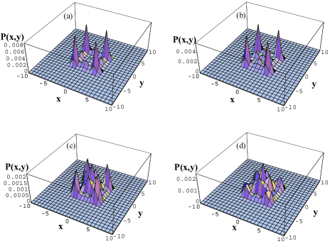
Figure 1: (Color online) The joint position distribution for a two-walker QW on a line after $t=6$ steps with various SWAP-operator powers: (a) $\tau=0$, (b) $\tau=0.5$, (c) $\tau=0.8$, and (d) $\tau=1$.

For the power of the SWAP operation $\tau=0$, which means the two walkers are uncorrelated, $P(x,y;t)$ is simply the product of the two independent one-walker distributions, $P_{1}(x;t)P_{2}(y;t)$, where $P_{1}(x;t)$ is the probability distribution for finding walker $1$ in position $x$ after $t$ and similarly for $P_{2}(y;t)$ and walker $2$.

The correlation functions $P(x,y;t=6)$ are shown in Fig. 1, The products of two independent single-walker distributions is evident in Fig. 1, which shows the $\tau=0$ case. However, for $\tau>0$, the walkers are not independent of each other due to the walkers (fractionally) swapping their coins after each step.

Evidently the SWAP operation on the two coins correlates and perhaps entangles the two coins. For classical RWs, the correlation between the coins do not affect the walkers behavior and the position distribution of each walker keeps the same as that of a standard RW with one walker. Compared to RWs, the interference effect and entanglement between each walker and his coin make the two-walker QW behave differently. The correlation between the coins is transferred to the walkers thereby inducing correlation between the two walkers. However, the interference effect and entanglement between each walker and his coin is partially destroyed by the SWAP operation.

In Fig. 1, the joint position distributions of two walkers after the $6^{\text{th}}$ step with various powers $\tau$ of the SWAP operation $\tau$ displays key concepts. For $\tau=0$, the two walkers are completely independent. For increasing $\tau$, a small peak appears in the middle of the distribution, which means there is correlation between the two walkers. For $\tau=1$, the peak in the middle gets large and the distribution still shows the quantum behavior of two walkers. Thus the correlation between two walkers increases with increasing power $\tau$ of the SWAP operation.

III.2 Mutual information and quantum mutual information

In probability theory and information theory, the mutual information of two random variables quantifies mutual dependence of the two random variables. Here we use the mutual information as a measure of classical correlation between two quantum walkers fractionally swapping their coins. Formally the mutual information of the positions of the two walkers can be defined as

$$I_{\text{c}}(t)=\int\int P(x,y;t)\log_{2}\left[\frac{P(x,y;t)}{P_{1}(x;t)P_{2}(y;t)}\right]\text{d}x\text{d}y.$$ (36)

As there is no classical correlation, the mutual information of two independent walkers is zero.

The SWAP operation between two coins connects the two walkers and introduces correlations. We use the mutual information as a measure of classical correlations between two walkers. In Fig. 2 the mutual information of the two walkers’ positions is depicted for various powers of the SWAP operation $\tau$.

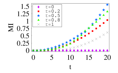
Figure 2: (Color online) The mutual information (MI) for the positions of the two walkers as a function of time $t$ with various choices of the SWAP operator power $\tau$.

In the case of $\tau=0$, the two walkers, each holding an independent Hadamard coin, walk on a separate line independently of the other’s dynamics so the mutual information of the two walkers’ positions is necessarily zero.

For a classical RW, if two walkers exchange their coin after every step, any correlation between each walker and his coin is severed. However, for the QW, correlations between the two walkers are not completely destroyed. For $\tau=1/2$ the two coins are maximally entangled by the $\sqrt{\text{SWAP}}$ operation, thereby maximizing the correlation between the two walkers.

In addition to classical correlations, the SWAP operation on two coins introduces quantum correlations between the two walkers as well. Now we consider the total correlation between two quantum walkers on a line under the influence of the SWAP operation between the coins. We use the quantum mutual information as a measure of the total correlation including classical and quantum correlations L08 ; LL07 ; L03 ; L06 ; OZ01 ; V03 ; M10 ; GBB10 between the walkers.

Given a bipartite state $\rho_{\text{w}}$ and the reduced density matrices denoted by $\rho_{1}$ and $\rho_{2}$, the quantum mutual information,

$$I\left[\rho_{\text{w}}(t)\right]=S\left[\rho_{1}(t)\right]+S\left[\rho_{2}(t)\right]-S\left[\rho_{\text{w}}(t)\right],$$ (37)

is a reasonable measure for total correlation between systems $1$ and $2$, where $S(\bullet)$ denotes von Neumann entropy. The quantum mutual information can be interpreted analogously to the classical case, namely

$$I\left[\rho_{\text{w}}(t)\right]=S\left[\rho_{\text{w}}(t)\|\rho_{1}(t)\otimes\rho_{2}(t)\right],$$ (38)

where $S(\bullet\|\bullet)$ denotes quantum relative entropy. Intuitively, the quantum mutual information reports the shared quantum information between walkers $1$ and $2$.

Quantum mutual information is a good measure for quantifying the reduction of the uncertainty of one variable through knowing the other variable. For example, if walkers $1$ and $2$ are independent, then knowing walker $1$’s position does not give any information about $2$’s position and vice versa so their quantum mutual information is zero. Otherwise, if walkers $1$ and $2$ are correlated, the quantum mutual information is positive, and the bound on this correlation is approximately $2\log_{2}d$ with $d$ the dimension of the walker state.

The total correlation between two walkers increases with the powers $\tau$ of the SWAP operations as does the classical correlation. Figure 3 presents plots of the quantum mutual information for an evolving two-walker QW system with various powers of the SWAP operation.

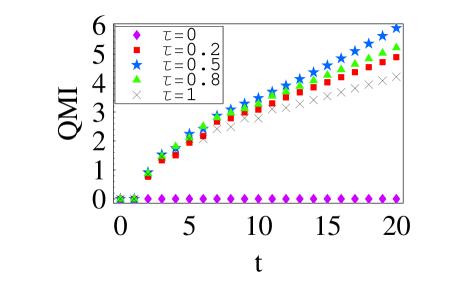
Figure 3: (Color online) The quantum mutual information (QMI) for two walkers’ positions as a function of time $t$ with various powers of the SWAP operator $\tau\in\left[0,1\right]$.

For fixed value of $\tau$, the quantum mutual information increases monotonically as the number of the steps increases. For $\tau=0$, the quantum mutual informations stays at zero, which means the total correlations are cut off between the two walkers. The quantum mutual informations for $\tau>0$ are positive and a maximum for $\tau=1/2$. We can see the maximal correlation (both total correlation and classical correlation) between walkers where we expect to see the coins entangled maximally.

III.3 Quantum correlations

Quantum discord OZ01 is a popular measure for characterizing purely quantum correlations within a bipartite state, but evaluating quantum discord requires extremizing over local measurement strategies. Such an evaluation can be intractable so measurement-induced disturbance was proposed as an operational measure that avoids such an onerous optimization. measurement-induced disturbance relies on diagonalizing the reduced density operators, which is tractable for small systems. For standard QWs, measurement-induced disturbance acts as a loose upper bound on quantum discord and tends to reflect well behavioral trends of the quantum discord SBC10 .

Measurement-induced disturbance and quantum discord have been compared for noisy linear and cyclic QWs RSCB11 . Whereas measurement-induced disturbance has an operational definition, operational meaning for quantum discord is less straightforward CAB+11 . On the other hand measurement-induced disturbance tends to overestimate non-classicality because it does not optimize over local measurements. Despite this over-estimation, measurement-induced disturbance gives a loose upper bound on quantum discord and reflects well quantum correlations for QWs RSCB11 . Nevertheless, care is need in interpretations of quantum correlations from measurement-induced disturbance as regimes exist where lack of optimization leads to overestimates of non-classicality.

Given the reduced two-walker bipartite state $\rho_{\text{w}}$ (tracing over coins), let the reduced density matrices for the two walkers be diagonalized to

$$\rho_{i}=\sum_{j}p_{i}^{j}\Pi_{i}^{j},$$ (39)

for $i=1,2$, where $\{\Pi_{i}^{j}\}$ is a complete projection-valued measure (i.e. using von Neumann measurements) for each $i$. Summing over joint projections on the two-walker state yields the diagonalized state

$$\Pi\rho_{\text{w}}(t)=\sum_{j,k}\Pi_{1}^{j}\otimes\Pi_{2}^{k}\rho_{\text{w}}(t)\Pi_{1}^{j}\otimes\Pi_{2}^{k}.$$ (40)

The leftmost $\Pi$ is an operator on the density matrix that diagonalizes it in the spectral basis corresponding to $\Pi_{i}^{j}$ projective measurements. The operator $\Pi$ can also be described as a ‘local measurement strategy’.

Correlations between the two reduced-walker states $\rho_{1}$ and $\rho_{2}$ are regarded as classical if there is a unique local measurement strategy $\Pi$ leaving $\Pi\rho_{\text{w}}(t)$ unaltered from the original two-walker state $\rho_{\text{w}}$ L08 . We ascertain whether the reduced two-walker state is ‘quantum’ by determining whether a local measurement strategy exists that leaves the two-walker state unchanged.

The degree of quantumness is given by the measurement-induced disturbance L08

$$Q\left[\rho_{\text{w}}(t)\right]=I\left[\rho_{\text{w}}(t)\right]-I\left[\Pi\rho_{\text{w}}(t)\right],$$ (41)

for $I(\bullet)$ the quantum mutual information. By construction $\Pi\rho_{\text{w}}(t)$ is classical. Hence $I\left[\Pi\rho_{\text{w}}(t)\right]$ quantifies the classical correlations in $\rho_{\text{w}}(t)$, which must equal $I_{c}$ (36). Thus, the measurement-induced disturbance is the difference between the quantum and classical mutual information, which quantify total and classical correlations. Accordingly, Eq. (41) is interpreted as the difference between the total and classical correlations, which are represented by the quantum mutual information and the mutual information.

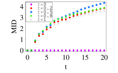
Figure 4: (Color online) The measurement-induced disturbance (MID) for two walkers’ positions as a function of $t$ with various powers of the SWAP operation $\tau\in\left[0,1\right]$.

Figure 4 presents plots of measurement-induced disturbance of two walkers in a two-walker QW system. From the relationship between total, classical and quantum correlations discussed in the previous paragraph, we expect a tight quantitative relationship between Figs. 2, 3 and 4. We see that the total correlation represented by quantum mutual information in Fig. 3 dwarfs the classical correlation represented by mutual information in Fig. 2. Hence Figs. 3 and 4 are quite similar.

Pure quantumness, represented by the measurement-induced disturbance depicted in Fig. 4, is monotonically increasing with $\tau$, and pure quantum correlations thus exist between the two walkers. This pure quantum correlation is not due to direct walker-walker interactions but are rather due to the walkers fractionally swapping their coins after each step, and the pure quantum correlations survive the tracing out of these coins.

IV Conclusions

We analyze the dynamics and entanglement of two quantum walkers who fractionally swap (i.e. perform a SWAP^τ unitary operation with $0\leq\tau\leq 1$) coins. We use mutual information, quantum mutual information and measurement-induced disturbance as measures to isolate classical vs quantum correlations.

Quantum discord would be a valuable measure to use but is not tractable in our case. However, measurement-induced disturbance suffices to show that pure quantum correlations are induced by having the walkers fractionally swap coins and then tracing out the degrees of freedom for the two coins. In fact both classical and quantum correlations co-exist between the two walkers for $\tau>0$. Quantum correlations are strongest for $\tau=1/2$ where the $\sqrt{\text{SWAP}}$ has maximal entangling power and is applied after each step.

Fractional swapping is a quintessentially quantum process. Classically the walkers can swap their coins or not, or they could SWAP their coins sometimes, either deterministically or probabilistically. In our two-walker fractional-coin-swapping scenario, a fractional coin swap is effected after every step identically. Classically one would expect that coin swapping would not affect the dynamics anyway because the coin state is unimportant: the flip chooses a random outcome. Our classical understanding of coin swapping thus gives little intuition about the quantum case. Thus, our analysis is quite valuable in that we characterize this two-walker fractional-coin-swapping case carefully and devise appropriate, tractable, meaningful classical and quantum correlation measures to study entanglement for this system.

- (1) Y. Aharonov, L. Davidovich and N. Zagury, Phys. Rev. A48, 1687 (1993).
- (2) D. Aharonov, A. Ambainis, J. Kempe and U. Vazirani, Proc. 33rd STOC (New York) pp 50-59 (2001).
- (3) V. Kendon, Phil. Trans. R. Soc. A 364, 3407 (2006).
- (4) T D Mackay, S D Bartlett, L T Stephenson and B C Sanders, J. Phys. A: Math. Gen. 35, 2745 (2002).
- (5) C. Di Franco, M. Mc Gettrick, and Th. Busch, Phys. Rev. Lett. 106, 080502 (2011).
- (6) C. Di Franco, M. Mc Gettrick, T. Machida, and Th. Busch, Phys. Rev. A84, 042337 (2011).
- (7) T. Brun, H. A. Carteret and A. Ambainis, Phys. Rev. A 67, 052317 (2003).
- (8) T. Brun, H. A. Carteret and A. Ambainis, Phys. Rev. Lett. 91, 130602 (2003).
- (9) M. Stefanak, S. M. Barnett, B. Kollar, T. Kiss and I. Jex, New J. Phys. 13, 033029 (2011).
- (10) P. P. Rohde, A. Schreiber, M. Stefanak, I. Jex and C. Silberhorn, New J. Phys. 13, 013001 (2001).
- (11) A. Ahlbrecht, H. Vogts, A. H. Werner and R. F. Werner, J. Math. Phys. 52, 042201 (2011).
- (12) A. Ahlbrecht, A. Alberti, D. Meschede, V. B. Scholz, A. H. Werner and R. F. Werner, Preprint: arXiv:1105.1051.
- (13) S. D. Berry and J. B. Wang, Phys. Rev. A83, 042317 (2011).
- (14) M. Mohseni, P. Rebentrost, S. Lloyd and A. Aspuru-Guzik, J. Chem. Phys. 129, 174106 (2008).
- (15) B. C. Travaglione and G. J. Milburn, Phys. Rev. A 65, 032310 (2002).
- (16) P. Xue and B. C. Sanders, New J. Phys. 8, 053025 (2008).
- (17) P. Xue, B. C. Sanders, A. Blais and K. Lalumière, Phys. Rev. A 78, 042334 (2008).
- (18) F. Helmer, M. Mariantoni, A. G. Fowler, J. von Delft, E. Solano and F. Marquardt, Euro. Phys. Lett. 85, 50007 (2009).
- (19) W. Dür. R. Raussendorf, V. M. Kendon and H. J. Briegel, Phys. Rev. A 66, 052319 (2002).
- (20) J. Kempe, Contemp. Phys. 44, 307 (2003); N. Shenvi, J. Kempe and K. B. Whaley, Phys. Rev. A 67, 052307 (2003).
- (21) J. P. Keating, N. Linden, J. C. F. Matthews and A. Winter, Phys. Rev. A76, 012315 (2007).
- (22) A. Schreiber, K. N. Cassemiro, V. Potoček, A. Gábris, I. Jex, and Ch. Silberhorn, Phys. Rev. Lett. 106, 180403 (2011).
- (23) H. Ollivier and W. H. Zurek, Phys. Rev. Lett. 88, 017901 (2001).
- (24) S. Luo, Phys. Rev. A77, 022301 (2008).
- (25) N. Li and S. Luo, Phys. Rev. A 76, 032327 (2007).
- (26) S. Luo, Phys. Rev. A 77, 042303 (2008).
- (27) S. Luo, Phys. Rev. A 73, 022324 (2006).
- (28) V. Vedral, Phys. Rev. Lett. 90, 050401 (2003).
- (29) K. Modi, T. Paterek, W. Son, V. Vidal and M. Williamson, Phys. Rev. Lett. 104, 080501 (2010).
- (30) O. Giraud, P. Braun and D. Braun, New J. Phys. 20, 063005 (2010).
- (31) R. Srikanth, S. Banerjee and C. M. Chandrashekar, Phys. Rev. A81, 062123 (2010).
- (32) B. R. Rao, R. Srikanth, C. M. Chandrashekar and S. Banerjee, Phys. Rev. A83, 064302 (2011).
- (33) D. Cavalcanti, L. Aolita, S. Boixo, K. Modi, M. Piani and A. Winter, Phys. Rev. A83, 032324 (2011).