A Bayesian Joinpoint regression model with an unknown number of break-points

Abstract

Joinpoint regression is used to determine the number of segments needed to adequately explain the relationship between two variables. This methodology can be widely applied to real problems, but we focus on epidemiological data, the main goal being to uncover changes in the mortality time trend of a specific disease under study. Traditionally, Joinpoint regression problems have paid little or no attention to the quantification of uncertainty in the estimation of the number of change-points. In this context, we found a satisfactory way to handle the problem in the Bayesian methodology. Nevertheless, this novel approach involves significant difficulties (both theoretical and practical) since it implicitly entails a model selection (or testing) problem. In this study we face these challenges through (i) a novel reparameterization of the model, (ii) a conscientious definition of the prior distributions used and (iii) an encompassing approach which allows the use of MCMC simulation-based techniques to derive the results. The resulting methodology is flexible enough to make it possible to consider mortality counts (for epidemiological applications) as Poisson variables. The methodology is applied to the study of annual breast cancer mortality during the period 1980–2007 in Castellón, a province in Spain.

, and

T1Supported in part by Ministerio de Educación y Ciencia; Contract Grants MTM2007-61554, MTM2010-19528.

T2Supported in part by Fondo de Investigaciones Sanitarias. Instituto de Salud Carlos III; Contract Grant ISCIII06-PI1742.

1 Introduction

Joinpoint regression is a statistical modeling technique that explains the relationship between two variables by means of a segmented linear regression constrained to be continuous everywhere, in particular, in those places where the slope of the regression function changes. This technique is widely applied to the modeling of time trends in mortality or incidence series in epidemiological studies. In these applications the number (if any) and the location of the changes in trends (known as change-points or joinpoints) is usually unknown, the main goal being to assess their existence and determine their location. Joinpoint regression is applied in a wide variety of contexts. Nevertheless, for clarity of presentation of the main ideas in this paper, the above-mentioned epidemiological setting is assumed throughout the paper.

The underlying problem in this context is a model selection (or testing) problem, with uncertainty about which is the model (number of change-points) that (most likely) produced the data observed. In this paper we approach the problem from a Bayesian perspective which is fully detailed below. Nevertheless, the predominant techniques in the context of Joinpoint regression are frequentist. Within them, the main goal is to find “the smallest number of joinpoints such that, if one more joinpoint is added, the improvement is not statistically significant” [Statistical Research and Applications Branch, National Cancer Institute (2009)]. This goal is usually met by means of nonparametric permutation tests [Kim et al. (2000)], the final result of that analysis being the determination of the model that meets the former condition and the estimation of its parameters and their variability. The National Cancer Institute (NCI) of the United States has developed a tool to carry out these kinds of analyses [Statistical Research and Applications Branch, National Cancer Institute (2009)]. This software has become a standard tool in epidemiological literature; see, for example, Cayuela et al. (2004), Bosetti et al. (2005), Stracci et al. (2007), Karim-Kos et al. (2008), Bosetti et al. (2008), Qiu et al. (2009).

The proposed permutation test approach has, in our opinion, two main limitations:

[(ii)]

The underlying model selection criterion selects the simplest model such that if a new joinpoint is added, it does not yield a statistically significant improvement. Therefore, the model selected is not the most likely one, but it is chosen according to both its capacity to describe the time trend within the data and the informativeness of data to highlight temporal changes (in the case of mortality or disease incidence time series, this last feature will depend heavily on the average number of annual observed cases in the data set). Hence, in a situation when the data is not very informative, the criteria is clearly biased (by definition) toward more simplistic models. This conservative behavior of the permutation procedure could seem reasonable to some authors [Kim, Yu and Feuer (2009)], but we find this systematic tendency unsatisfactory. Instead, in this situation we would expect to be “informed” that a number of alternative models are equally plausible.

It is hard to quantify to what extent one selected model is more likely than others. In practice, a single model is chosen, with a fixed number of joinpoints, regardless of whether the choice is much more likely or not than the other alternatives. As a consequence, the main goal of the inference in these kinds of models (how many joinpoints can adequately explain the time trend that we are observing?) lacks an estimate of its variability in contrast to the remaining parameters of the selected model. This is because the asymptotics of the number of joinpoints is an involved issue. Relevant advances in this regard include the work of Yao (1988), Liu, Wu and Zidek (1997), Kim, Yu and Feuer (2009), focusing mainly on conditions where estimators of this parameter are consistent (converge to the parameter as the sample size increases).

There is some previous work devoted to the application of Bayesian ideas to Joinpoint problems. Carlin, Gelfand and Smith (1992) is one of the pioneering contributions in this area, proposing the application of MCMC methods to fit these kinds of models. Moreno, Torres and Casella (2005) derived the intrinsic priors for a possibly heteroscedastic normal model under the assumption of a fixed change-point. In a similar problem but under homoscedasticity, more recently, Bayarri and García-Donato (2007) explicitly derived the Zellner–Siow priors [Zellner and Siow (1980); Zellner (1984)]. Bearing in mind its epidemiological application, Tiwari et al. (2005) describe the calculus of Bayes factors for model selection in Gaussian joinpoint models. A common limitation of the application of all these studies to epidemiological time series modeling is the assumption of normal errors. This restriction is relaxed in the work of Ghosh, Basu and Tiwari (2009), who propose semiparametric regression models by means of Dirichlet processes. Nevertheless, the original data in mortality studies are usually the annual observed death counts, for which in this paper we assume a Poisson regression model to take into account the discrete nature of these data. As far as we know, the only Bayesian model selection approach that considers Poisson counts in the context of Joinpoint regression is Ghosh et al. (2009). These authors also acknowledge the advantage of the Poisson assumption especially when the observed counts are smaller, in which case the Gaussian modeling of incidence or mortality rates is clearly not convenient. That is probably the work most closely related to ours. Nevertheless, our approach differs from it in at least two main ways. First, Ghosh et al. (2009) model the hazard rate in a context of relative survival, while we propose a model for the, more usual in this context, incidence or death rates (see Section 3.1). Second, the model selection performed in Ghosh et al. (2009) is based on popular model selection criteria like CPO and DIC, but not on posterior probabilities as we do. The advantages of posterior probabilities over other criteria are a straightforward interpretation and the richness of the results produced (e.g., to produce predictions). These are put in practice in Section 4.

The Bayesian approach is straightforward at least conceptually. Bayes factors allow the selection of models from among several alternatives, strictly according to their posterior probabilities. Furthermore, through Bayes factors it is possible not only to select one of the models entertained, according to the evidence (posterior probability) provided by the data, but also to quantify the difference between the one selected and the remaining competing models. In a broad sense, Bayes factors make it possible to evaluate the uncertainty involved with the selection made. Furthermore, their use is the basis for what has been called Model Averaging [Clyde (1999)], under which it is possible to average the fit of all the models weighted by their posterior probabilities. Therefore, uncertainty in the selection of the “correct” model is propagated to the inferential exercise.

The goal of this study is to propose a Joinpoint regression modeling that evaluates and incorporates the uncertainty in both model selection and model parameters into the analysis. We found the Bayesian approach, for the aforementioned reasons, a very appealing way of doing so. Of course, the Bayesian approach to model selection problems is not free of difficulties, as nicely explained in Berger and Pericchi (2001). These can basically be summarized in two main problems: a strong influence of the prior on the results and a very challenging numerical problem to compute these results. Much of the material presented in this paper focuses on how we manage to overcome these problems.

The rest of the paper is organized as follows: Section 2 introduces a reparameterization of the usual Joinpoint regression model which will be really convenient as a first step to assign prior distributions. In Section 3, starting from the reparameterization proposed in Section 2, we introduce a Joinpoint modeling proposal with an unknown number of change-points. That proposal will be carried out as a variable selection process [George and McCulloch (1993); Dellaportas, Forster and Ntzoufras (2000, 2002)], and prior distributions will be discussed in detail in order to get reasonable results from the previous model selection problem. In Section 4 our new model will be applied to the study of breast cancer mortality in the Spanish province of Castellón to illustrate the possibilities of the Bayesian approach for exploiting the results from the inference. Finally, in Section 5 we will summarize the main advances of our model and some future lines of work will be outlined.

2 A convenient parameterization of the joinpoints

Suppose that we want to describe the behavior of the variable $\{Y_{i};i=1,\ldots,n\}$ as a function of the explanatory covariate $\{t_{i},i=1,\ldots,n\}$. We find it convenient to assume that $t_{i}$ represents time, although it could represent any other magnitude. It is usual to model the presence of $J$ change-points (locations in which the functional describing the relationship between $Y$ and $t$ changes) through the expected value of the dependent variable as

$$g(E(Y_{i}|t_{i}))=\alpha+\beta_{0}\cdot t_{i}+\sum_{j=1}^{J}\beta_{j}\cdot(t_{i}-\tau_{j})^{+}$$ (1)

for certain $g$, a linking function. In this equation, $\tau_{j}$ represents the location of the $j$th change-point and $(\theta)^{+}$ is $\theta$ if $\theta>0$, and 0 otherwise. We label the model in (1) as $M_{J}$, to make it explicit that it contains exactly $J$ change-points. Similarly, we call the model with no change-points $M_{0}$.

In what follows, we assume that the maximum number of change-points is $J^{*}$, a number which is fixed (more on this aspect later). Then the problem that we face is to find the posterior probability of each of the models in $\{M_{0},M_{1},\ldots,M_{J^{*}}\}$ and in the case that a single model needs to be selected, the one with the highest posterior probability is preferred.

In the Bayesian framework, the distinction between common and new parameters for the assignment of prior distributions [first used by Jeffreys (1961)] is crucial. The terminology is very intuitive: common parameters appear in all the competing models while the new parameters are model-specific. In the problem above, $\alpha$ and $\beta_{0}$ are common and the remaining $\beta$’s are new parameters.

As we fully describe in the following section, the scheme that we adopt for the assignment of the priors proposes the same marginal (noninformative) prior for the common parameters. Clearly, using the same prior (either subjectively elicited or not) for common parameters does not make sense unless the meaning of these parameters does not change throughout the different models entertained. Unfortunately, common parameters do not (in general) represent the same magnitude, this being a major difficulty in Bayesian model selection [see Berger and Pericchi (2001)]. Although it is hard to establish precise conditions under which common parameters have the same meaning (a notion which can be viewed as subjective), it is clear that, as it stands, this is not the case for the problem presented above. For instance, in $M_{0}$, $\alpha$ and $\beta_{0}$ represent the parameters explaining the global trend of the series. Nonetheless, in $M_{1}$ (a model with one joinpoint) $\alpha$ and $\beta_{0}$ are the intercept and the slope respectively of a line adjusted up to the change-point ($\tau_{1}$), $\beta_{0}+\beta_{1}$ being the slope from the joinpoint on. We propose an alternative parameterization, for which we argue that the hypothesis of common parameters with a same meaning across models holds reasonably. More concisely, let

$$E(Y_{i}|t_{i})=\alpha+\beta_{0}\cdot(t_{i}-\bar{t})+\sum_{j=1}^{J}\beta_{j}\mathcal{B}_{\tau_{j}}(t_{i}),$$ (2)

where $\mathcal{B}_{\tau_{j}}(t)$, which we call the break-point or the break-point centered at $\tau_{j}$, is defined as the following piecewise linear function:

$$\mathcal{B}_{\tau_{j}}(t)=\cases{\displaystyle a_{0j}+b_{0j}\cdot t,&\quad$\forall t\leq\tau_{j}$,\cr\displaystyle a_{1j}+b_{1j}\cdot t,&\quad$\forall t>\tau_{j}$,}$$

restricted to a number of conditions which are fully specified below. What we finally obtain is, conditioned on the joinpoints, a known function of the original regressors at times $\{t_{1},t_{2},\ldots,t_{n}\}$ and describing a peak at the moment $\tau_{j}$. Alternatively, the set of break-points can be interpreted as a base of continuous piecewise linear functions generating the joinpoints needed to describe the time trend in the data. The linear component in (2) has been introduced as $(t_{i}-\bar{t})$ (instead of $t_{i}$) to avoid the dependency between $\alpha$ and $\beta_{0}$.

The conditions imposed on $\mathcal{B}_{\tau_{j}}(t)$ are as follows:

• $\lim_{t\to\tau_{j}^{-}}\mathcal{B}_{\tau_{j}}(t)=\lim_{t\to\tau_{j}^{+}}\mathcal{B}_{\tau_{j}}(t)$, that is, $\mathcal{B}_{\tau_{j}}(t)$ is a continuous function. Hence, it is guaranteed that the regression function (2) is continuous all around, independently of the number of break-points.

• $\sum_{i=1}^{n}\mathcal{B}_{\tau_{j}}(t_{i})=0$, that is, the sum of the elements of the break-point evaluated in all the points observed must be zero. This way the addition of any break-point in the model would not alter the mean value of the regression function and it would not change the meaning and the estimation of parameter $\alpha$ across models. In other words, this condition can be understood as if the new break-points are imposed to be geometrically orthogonal to the intercept term.

• $\sum_{i=1}^{n}\mathcal{B}_{\tau_{j}}(t_{i})\cdot t_{i}=0$, that is, the slope of the break-points along the whole period of study is zero. This way the addition of any break-points in the model would neither alter the slope of the regression function nor would it change the meaning and the estimate of parameters $\beta_{0}$ across models. In other words, this condition can be understood as if the new break-points are imposed to be geometrically orthogonal to the slope term.

• $\mathcal{B}_{\tau_{j}}(\tau_{j})=1$, so that the parameter $\beta_{j}$ has the role of measuring the magnitude of the break-point in the location where the change in the tendency takes place. Hence, $\beta_{j}$ has to be interpreted as the value of the deviation produced at $\tau_{j}$ as a consequence of including this break-point in the model. Without a restriction of this kind the value of $\beta_{j}$ would not be identifiable.

Subject to these conditions and given $\tau_{j}$, the function $\mathcal{B}_{\tau_{j}}(t)$ is unambiguously determined (details are provided as supplementary material [Martinez-Beneito, Garcia-Donato and Salmerón (2011)]).

The main motivation for introducing the above basis of functions is to improve robustness over prior specification by reparameterization as is further explained below. In this sense, our approach is different from the other basis of functions used [like MARS in Friedman (1991) and Nott, Kuk and Duc (2005)] where the aim was to approximate surfaces which could potentially be highly nonlinear on their multiple arguments. With this parameterization, it is now reasonable to assume that the common parameters have the same meaning: in all models, $\alpha$ and $\beta_{0}$ are parameters of a line representing the global trend. The remaining parameters are used to modify this common line to incorporate changes in the trend without changing the original meaning of $\alpha$ and $\beta_{0}$ in $M_{0}$.

As an illustration, a graphical representation of several break-points, corresponding to different locations of the change-points (for 20 observed values), is shown in Figure 1 (left). As can clearly be seen, all break-points are equal to 1 at their corresponding change-points, are zero on average and their slope is also null. Following this same context, Figure 1 (right) shows how the inclusion of break-points modifies a straight line common to all models ($\alpha+\beta_{0}\cdot t$). In this figure we have plotted the line $y(t)=10+0.1\cdot t$, jointly with the functions $y(t)=10+0.1\cdot t+0.5\cdot\mathcal{B}_{5}(t)$ and $y(t)=10+0.1\cdot t+0.5\cdot\mathcal{B}_{5}(t)-0.3\cdot\mathcal{B}_{13}(t)$. The effect of including break-points over a common regression function is the torsion of this function, instead of a divergence from a certain place as was done in the parameterization in (1). In other words, the effect of the introduced break-points is a global modification of the regression curve, as opposed to the previous parameterization which produced a local modification, changing the meaning of the parameters $\alpha$ and $\beta_{0}$ depending on whether the break-points are (or are not) included in the model and how many of them are included.

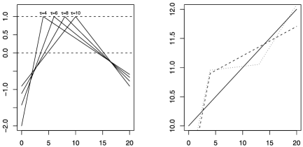
Figure 1: Left: Shape of different break-points as a function of their change-point locations. Right: Trends with 0 (solid line), 1 (dashed line) and 2 (dotted line) change-points. All these functions have the same mean value and slope for the whole period.

Additionally, a number of nice side effects are derived from this parameterization:

• With the definition of the break-points, the columns of the design matrix corresponding to the common parameters are orthogonal to the columns of the new parameters. Hence, we can reasonably expect the Fisher information to be approximately block diagonal (of course, it depends on the particular distribution assumed for $Y$, and will be true for the normal case). In this scenario, it is known that the Bayes factors (and consequently any other result derived from them, like the posterior probabilities) are quite robust to the prior distribution used for common parameters [see Jeffreys (1961); Kass and Vaidyanathan (1992)]. This has been used as a justification for the strategy of using noninformative priors, possibly improper, for common parameters [see Liang et al. (2008); Bayarri and García-Donato (2008)]. We use a similar approach, as we explain in the next section.

• With this reparameterization, the common parameters $\alpha$ and $\beta_{0}$ conserve their meaning regardless of the model (i.e., regardless of the number of joinpoints). This allows us to make inferences about them in a model-averaged way, that is, taking into account the uncertainty regarding which is the true model. We put this into practice in Section 4 where we draw inferences on these parameters.

3 A Joinpoint regression model with an unknown number of change-points

3.1 An encompassing model

To address the question of how many joinpoints are needed, or, equivalently, to select from among $\{M_{0},M_{1},\ldots,M_{J^{*}}\}$, we introduce an encompassing model in which all these models are nested. We also assume the scenario of modeling epidemiological series of mortality or incidence counts of a certain disease, since this is the most extended application of Joinpoint models. Nevertheless, the main ideas that we present hold for other types of data, not necessarily counting data.

Let $Y_{i}$ be the number of cases of a specific disease observed during a period of time, represented by $t_{i}$. To account for the discrete nature of these values, we suppose that

$$Y_{i}\sim\operatorname{Poisson}(\mu_{i}),\qquad i=1,\ldots,n,$$

whose mean is defined as

$$\log(\mu_{i})=\log(P_{i})+\alpha+\beta_{0}\cdot(t_{i}-\bar{t})+\sum_{j=1}^{J^{*}}\delta_{j}\cdot\bigl{(}\beta_{j}\cdot\mathcal{B}_{\tau_{j}}(t_{i})\bigr{)},$$ (3)

where $P_{i}$ is the population under study during year $i$, $\{\delta_{j};j=1,\ldots,J^{*}\}$ are binary variables which include (for $\delta_{j}=1$) or exclude (for $\delta_{j}=0$) each change-point in the model and $\tau_{j}$ is the unknown location of the $j$th break-point. This model can be interpreted as an encompassing model, which contains all possible joinpoint models unambiguously identified through $\bolds{\delta}=(\delta_{1},\ldots,\delta_{J^{*}})$, to explain the data. In particular, $M_{0}\equiv\{\bolds{\delta}=\bolds{0}\}$, $M_{1}\equiv\{\bolds{\delta}\dvtx\allowbreak\sum_{j=1}^{J^{*}}\delta_{j}=1\},\ldots$ and $M_{J^{*}}\equiv\{\bolds{\delta}=\bolds{1}\}$. Hence, the posterior probability over the model space $\{M_{0},M_{1},\ldots,M_{J^{*}}\}$ is completely specified through the posterior distribution of $\bolds{\delta}$. A detailed description of the computation of $\pi(\bolds{\delta}|\mathbf{y})$ is provided as supplementary material [Martinez-Beneito, Garcia-Donato and Salmerón (2011)]. The proposal in (3) can in a way be seen as an order-2 regression spline [Hastie, Tibshirani and Friedman (2009)], as this is a piecewise linear continuous regression function.

To avoid identifiability problems, we impose a number of restrictions on the locations of the change-points on which there is broad consensus in the related literature. These are imposed so as to ensure a minimum distance between change-points and a restriction of order. In particular, we assume that the parametric space for $\bolds{\tau}=(\tau_{1},\tau_{2},\ldots,\tau_{J^{*}})$, which we call $\Omega$, is

$$\Omega=\{(\tau_{1},\ldots,\tau_{J^{*}})\dvtx t_{1}+d<\tau_{1},\tau_{1}+d<\tau_{2},\tau_{2}+d<\tau_{3},\ldots,\tau_{J^{*}}+d<t_{n}\}.$$

With this assumption, there is a minimum number of periods $d$ between any two change-points. By default, we use $d=2$ in our applications. Notice that this restriction avoids the existence of two or more change-points between consecutive observations. Other ways of implementing this restriction have been proposed, as, for example, in Ghosh, Basu and Tiwari (2009). Notice that $\Omega$ is a bounded set in ${\cal R}^{J^{*}}$.

3.2 The prior distribution

Let $\pi(\alpha,\beta_{0},\bolds{\delta},\bolds{\tau},\bolds{\beta})$ be the prior distribution of the parameters in the model (3). We express this prior as

$$\pi(\alpha,\beta_{0},\bolds{\beta},\bolds{\tau},\bolds{\delta})=\pi(\bolds{\beta}|\alpha,\beta_{0},\bolds{\delta},\bolds{\tau})\pi(\alpha,\beta_{0})\pi(\bolds{\tau})\pi(\bolds{\delta}),$$

where $\bolds{\beta}=(\beta_{1},\ldots,\beta_{J^{*}})$.

The prior $\pi(\alpha,\beta_{0})$ corresponds to common (with the same meaning, as argued in the previous section) parameters in all models. Under this condition, it is common to use a noninformative prior [see, e.g., Berger and Pericchi (2001); Bayarri and García-Donato (2007, 2008)], in this case the constant prior: $\pi(\alpha,\beta_{0})\propto 1.$

All the other parameters are not common and it is well known [Berger and Pericchi (2001)] that the posterior distribution is very sensitive to their prior distribution. In particular, noninformative (improper) or vague priors would produce arbitrary Bayes factors.

Our approach to assigning $\pi(\bolds{\beta}|\alpha,\beta_{0},\bolds{\delta},\bolds{\tau})$ is based on an approximation of the divergence based (DB) prior, introduced by Bayarri and García-Donato (2008) as a broad generalization of the pioneering ideas of Jeffreys (1961), Zellner and Siow (1980) and Zellner (1984). When comparing two nested models, an approximation of the DB prior for the new parameters in the complex model (possibly reparameterized to range within the real line) is a heavy tailed density, centered at zero and scaled by the inverse of the corresponding block of the unitary Fisher information matrix evaluated in the simpler model. This would lead us to the proposal

$$\pi(\bolds{\beta}|\alpha,\beta_{0},\bolds{\delta},\bolds{\tau})=\mbox{Cauchy}_{J^{*}}(\bolds{\beta}|\bolds{0},\bolds{\Sigma}),$$ (4)

the matrix $\bolds{\Sigma}$ to be specified. Using a hierarchical scheme, this is equivalent to the proposal

$$\pi(\bolds{\beta}|\alpha,\beta_{0},\bolds{\delta},\bolds{\tau},\gamma)=\mbox{Normal}_{J^{*}}(\bolds{\beta}|\bolds{0},\gamma\bolds{\Sigma}),\qquad\gamma\sim\operatorname{Gamma}^{-1}(0.5,0.5),$$

where $\gamma$ acts as a “mixing” parameter.

In our problem, it is easy to see that the block (corresponding to $\bolds{\beta}$) of the Fisher information matrix of the encompassing model (3) evaluated at $\bolds{\beta}=\bolds{0}$ is ${\cal I}=\bolds{\Delta}\mathbf{B}^{t}\mathbf{W}\mathbf{B}\bolds{\Delta}$, where $\mathbf{B}=\{B_{\tau_{j}}(t_{i})\}$ (the matrix of covariates), $\mathbf{W}=\operatorname{diag}\{w_{i}\}$ with $w_{i}=P_{i}\operatorname{exp}(\alpha+\beta_{i}(t_{i}-\bar{t}))$ and $\bolds{\Delta}=\operatorname{diag}(\bolds{\delta})$. Clearly, ${\cal I}$ is not (for every $\bolds{\delta}$) a positive-definite matrix, so it cannot be used directly to define $\bolds{\Sigma}$ above. Instead, we propose

$$\bolds{\Sigma}=n\bigl{(}\bolds{\Delta}\mathbf{B}^{t}\mathbf{W}\mathbf{B}\bolds{\Delta}+\operatorname{diag}(\mathbf{B}^{t}\mathbf{W}\mathbf{B}-\bolds{\Delta}\mathbf{B}^{t}\mathbf{W}\mathbf{B}\bolds{\Delta})\bigr{)}^{-1},$$ (5)

which is (for every $\bolds{\delta}$) a positive-definite matrix.

As we argue below, the resulting proposed prior (4) with a scale matrix as in (5) has a very interesting interpretation. Given a particular $\bolds{\delta}^{*}$, with, say, $\sum\delta_{i}^{*}=J$, let $\bolds{\beta}_{\delta}$ be the $J$-dimensional subvector of $\bolds{\beta}$ which corresponds to the nonnull $\delta_{i}$’s. Similarly, denote $\bolds{\beta}_{\delta^{c}}$ as the remaining parameters in $\bolds{\beta}$. Finally, $\mathbf{B}_{\delta}$ denotes the matrix with the columns in $\mathbf{B}$ which corresponds to the nonnull $\delta_{i}$’s. Hence, it can easily be seen that $\bolds{\beta}_{\delta}$ and $\bolds{\beta}_{\delta^{c}}$ are independent, conditional on the mixing parameter $\gamma$. In fact,

$$\pi(\bolds{\beta}|\alpha,\beta_{0},\bolds{\delta}=\bolds{\delta}^{*},\bolds{\tau},\gamma)=\mbox{Normal}_{J}(\bolds{\beta}_{\delta}|\bolds{0},\gamma n(\mathbf{B}_{\delta}^{t}\mathbf{W}\mathbf{B}_{\delta})^{-1})f(\bolds{\beta}_{\delta^{c}}|\alpha,\beta_{0},\bolds{\tau},\gamma),$$

where

$$f(\bolds{\beta}_{\delta^{c}}|\alpha,\beta_{0},\bolds{\tau},\gamma)=\prod_{\{i\dvtx\delta_{i}=0\}}\mbox{Normal}(\beta_{i}|0,\gamma n[\mathbf{B}^{t}\mathbf{W}\mathbf{B}]_{ii}^{-1}).$$

For every $\bolds{\delta}$, the joint prior $\pi(\bolds{\beta}|\alpha,\beta_{0},\bolds{\delta},\bolds{\tau})$ can be seen as the product of the (approximated) DB prior for the active parameters in the model, times a proper density for those inactive parameters. This proper density has no effect on the corresponding Bayes factors, thereby acting as a pseudoprior [see, e.g., Carlin and Chib (1995); Han and Carlin (2001); Dellaportas, Forster and Ntzoufras (2002)]. Nevertheless, as noticed previously in the literature, these may have a great impact on the numerical results. In our experience, partially described in the supplementary material [Martinez-Beneito, Garcia-Donato and Salmerón (2011)], this particular form of the pseudoprior leads to quite satisfactory results.

With this approach, the priors are in some sense defined encompassingly. That is, instead of using one (DB) prior for each possible submodel nested in (3), implicitly defined by each $\bolds{\delta}$, we use a single prior which contains all these priors. The main advantage of the resulting procedure is that it makes it possible (as we describe in the next section) to use standard estimation procedures (like MCMC) to easily solve the model selection problem, whose direct resolution usually requires the help of sophisticated numerical techniques.

The proposal for $\pi(\bolds{\tau})$ is not as delicate an issue as the prior for $\bolds{\beta}$. This is because the corresponding parametric space $\Omega$ is a bounded set which ensures that $\pi(\bolds{\delta})$ is proper under very mild conditions. Hence, the normalizing constant is unambiguously defined. In this situation, the constant prior is clearly a reasonable default choice: $\pi(\bolds{\tau})\propto 1$ for $\bolds{\tau}\in\Omega.$

Finally, we introduce our proposal for $\pi(\bolds{\delta})$, which is deeply related to our prior beliefs over the model space $\{M_{0},M_{1},\ldots,M_{J^{*}}\}$. One possibility would be to use independent Bernoulli distributions for $\delta_{i}$ with a probability of success of 0.5. Nevertheless, this would lead us to the $\operatorname{binomial}(J^{*},0.5)$ distribution over the model space, clearly favoring those models with around $J^{*}/2$ joinpoints and also giving an undesirable important role to the fixed value $J^{*}$ (which is usually posed as arbitrarily large).

Instead, we experimented with two different proposals. In the first one (which we refer to as Bayes1), all models $M_{i}$ have the same probability [i.e., $1/(J^{*}+1)$], this probability being equally distributed over the same number of joinpoints. This prior distribution can be formulated in a hierarchical way as

$$\pi(\bolds{\delta}|\mathbf{p})\propto\frac{\prod_{i=1}^{J^{*}}p_{i}^{\delta_{i}}(1-p_{i})^{(1-\delta_{i})}}{{J^{*}\choose\sum_{j=1}^{J^{*}}\delta_{j}}},\qquad\pi(p_{i})=\operatorname{Beta}(1/2,1/2),i=1,\ldots,J^{*}.$$

The term in the denominator of the prior for $\bolds{\delta}$ yields the same prior probability for any number of change-points in the model if $p_{1}=\cdots=p_{J^{*}}=0.5$ (the prior expected values of these terms). This hierarchical formulation, once the parameters $\mathbf{p}$ are integrated out, can also be expressed as

$$\pi_{1}(\bolds{\delta})=(J^{*}+1)^{-1}{\pmatrix{\displaystyle J^{*}\vspace*{2pt}\cr\displaystyle\sum_{j=1}^{J^{*}}\delta_{j}}}^{-1}.$$

The main drawback of this proposal is that, a priori, the mean number of joinpoints included in the model ($J^{*}/2$) depends on the arbitrary quantity $J^{*}$. While this is not a problem when $J^{*}$ is carefully assigned, it could be an issue when this parameter is arbitrarily assigned (as is the case in many studies). To avoid this dependency on $J^{*}$ as much as possible, while keeping the essence of the first proposal, we alternatively explore a slight modification on $\pi_{1}(\bolds{\delta})$. The prior (to be called Bayes2) can be defined hierarchically as

$$\pi(\delta_{i}|p_{i}) = \operatorname{Bernoulli}(p_{i}),\qquad i=1,\ldots,J^{*},$$

$$\pi(p_{i}) = \operatorname{Beta}\bigl{(}1/2,(J^{*}-1)/2\bigr{)},\qquad i=1,\ldots,J^{*}.$$

With this second proposal, the prior expected number of break-points(1 break-point) does not depend on the value of $J^{*}$.

In the same way as for Bayes1, this prior distribution can also be expressed in a nonhierchical way, once the $p_{i}$ parameters are marginalized, as

$$\pi_{2}(\bolds{\delta})=(J^{*})^{-J^{*}}(J^{*}-1)^{J^{*}-\sum_{j=1}^{J^{*}}\delta_{j}}.$$

Interestingly, as pointed out by an Associate Editor, for large $J^{*}$, the prior probability of zero and one joinpoint tends to $e^{-1}\approx 0.37$, emphasizing the robustness of $\pi_{2}$ to the choice of $J^{*}$.

4 Breast cancer mortality trend in Castellón province

We analyze the breast cancer mortality time trend in Castellón province, for the period 1980–2007. Castellón is one of the 50 provinces that make up Spain, where around 285,000 women resided in 2007 and with 62.4 women dying annually of breast cancer, on average, during that period. Two facts have occurred in those years that have presumably changed breast cancer mortality trends, which are the progressive introduction of the Breast Cancer Screening Program in that province in 1992 [Vizcaíno et al. (1998)], and the introduction of new therapies for the treatment of this disease around the world, at approximately the same time. In fact, there is some controversy over which of these two factors could have a higher impact on mortality variation [Peto (1996); Blanks et al. (2000); Berry et al. (2005)]. In any case, we would expect to find at least one joinpoint on the breast cancer mortality trend studied. Moreover, changes in breast cancer mortality trends have already been described for the first half of the 1990s for other Spanish regions [Ascunce et al. (2007); Salmerón et al. (2009); Pérez Lacasta et al. (2010)].

Regarding Bayesian criteria, if we focus on the mode of the posterior distribution of the number of joinpoints, in Figure 2 it can be seen that both methods point to the existence of exactly one joinpoint, indeed, Bayes1 yields a 51.0% probability of one joinpoint, while Bayes2 estimates that probability at 73.6%. Moreover, the probability of no joinpoint in the time trend for these two models is 1.9% and 3.0%, respectively. Hence, the probability of a “simply linear” trend for breast cancer mortality is low.

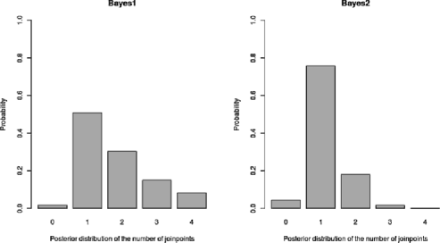
Figure 2: Posterior distribution of the number of joinpoints in breast cancer mortality trend in Castellón Province for Bayes1 and Bayes2 criteria.

On the other hand, we have used the Permutation and BIC criteria, by means of the NCI tool. The Permutation criterion (the one suggested by the NCI tool’s authors) does not find any joinpoints in the period under study, possibly due to the limited information on the trend provided by the low number of deaths by year. The BIC criterion, however, finds one joinpoint around 1995, with a 95% confidence interval: [1990, 2005]. As a consequence, the conservative behavior observed of the Permutation criterion makes it yield results which neither agree with the remaining criteria nor with the results that we expected, based on further knowledge of this cause of mortality. It has to be acknowledged that the Permutation test yields a $p$-value of 0.0136 when testing 1 versus 0 joinpoints, whereas the significance level of the test is 0.0125 (the result of the Bonferroni correction of the original level 0.05), that is, the model without any joinpoint is really close to being rejected. Therefore, the arguments for selecting between the models with either none or just one joinpoint are not conclusive at all for this example, but, on the contrary, the consequences derived from that selection are dramatic. This result warns against the danger of those criteria choosing a particular number of joinpoints and ignoring the uncertainty in that choice. In our example the permutation test would presumably have led to a wrong answer and from that moment on all the results from the analysis would have been completely missleading, as the premises of the chosen model are accepted as true and those from alternative models are completely ignored.

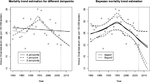
Figure 3: Left: Least squares estimated trends for a different number of joinpoints for the annual observed death rate (per 100,000 women). Right: Estimated time trend for the annual observed death rate (per 100,000 women) for both Bayes1 and Bayes2.

The left-hand side of Figure 3 shows the least squares estimated trend for a different number of joinpoints (recall that the Permutation test chooses the curve with 0 joinpoints from among all these). As can be noticed, fitted trends are quite different and the repercussion of the choice of one or another curve, and as a consequence of ignoring alternative models are dramatic. Those consequences could be even worse in the case of temporal forecasting. The former figure also shows the forecasted trend for every one of these curves for the following 5 years (2008–2012) and, as can be appreciated, predictions for the model without joinpoints diverge completely from those of the models with joinpoints. As the Permutation based criteria lacks an estimate of the probability of these scenarios, they cannot be averaged and one of them has to be chosen with the previously outlined risks. This is not the case of our proposed methods. The right-hand side of Figure 3 shows the estimated trend by both Bayes1 and Bayes2 where predictions based on different numbers of joinpoints are averaged to provide a single answer weighting all the scenarios considered. Moreover, as pointed out in George (1999), the predictions derived with this Model Averaging procedure are optimal in several senses, the square error loss being one of them. Predicted trends for both Bayesian criteria are really close, although the Bayes1 prediction depicts more detail than the Bayes2 as a consequence of the higher number of joinpoints that this model occasionally considers. From now on we will focus on the results of Bayes1 to improve the clarity of the presentation.

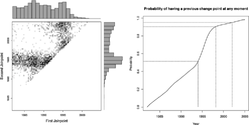
Figure 4: Left: Joint posterior distribution of the location of joinpoints conditioned to the model with just 2 joinpoints. Histograms correspond to the marginal posterior distribution of the location of the first and second joinpoint. Right: Probability of the trend having described a change-point before any specific moment.

The estimation of $\beta_{0}$ from Bayes1 yields a posterior mean of $-$0.0017 and a 95% probability interval $[-0.0077,0.0042]$. Consequently, the global trend during the whole period studied has a slope which is not very different from 0. The interest of this result is that it is valid regardless of the true number of joinpoints underlying the true trend, as we are not conditioning our results on a specific number of change-points. Conversely, the frequentist results condition all their conclusions on the selected model, and, therefore, they are valid if and only if that model agrees with the reality.

Figure 4 (left) shows the joint posterior distribution of the location of these two joinpoints. As can be noticed, this figure points out the existence of one joinpoint from about 1993 to 1997 and another one less precisely placed in the range from 1983 to 2005. For this second joinpoint there are several places that seem to be likely to host the second joinpoint. This information is much richer than that provided by the least squares estimate in Figure 3 that just points to 1987 as the most likely year for the second joinpoint. Focusing in the results in Figure 4 (left), our impression is that reducing the results of the 2-joinpoints-fit to a single curve (although it corresponds to the least squares fit) could be a really poor summary of all these results. Moreover, the marginal distribution of the locations of both joinpoints are multimodal and clearly asymmetric. Therefore, confidence intervals obtained for these quantities under asymptotic approximations will have to be treated with caution.

Finally, Figure 4 (right) shows, at every moment of the period under study, the probability of the trend having described a change-point before that precise moment. As it is evident that the curve converges to 0.981, the complement of the probability of not describing a joinpoint along the whole period of study. Moreover, from the start of 1994 the probability of already having described a joinpoint is higher than 50%, at the start of 1998 that probability is higher than 90% and we have to wait until 2002 to be sure, with a 95% probability, of having described at least one joinpoint. This way we can also measure (without any asymptotic assumptions) the degree of certainty that we have about the trend having described a change at any moment. It is possible to derive many posterior summaries of this kind with this approach. These will be able to answer most of the epidemiological questions that could be of particular interest in real studies.

5 Conclusions

This study has introduced a novel approach to Joinpoint analysis, taking advantage of considering the model selection problem as an inference problem on an encompassing model which contains all the candidate alternatives. Moreover, the possibility of carrying out its inference in WinBUGS is an important added value, as it makes it available to a wide community of users for further applications. We also think that the reparameterization made of the original problem has also been important, as it has made it possible to incorporate many previous model selection theory results. These results have given us a really valuable insight into the prior distributions of noncommon parameters, which is the main challenge from the Bayesian point of view, in order to give a reasonable answer to model selection problems.

Our proposal models the observed mortality as Poisson counts. This distributional assumption has several advantages: (i) it can cope with zero counts without any problem, (ii) no additional assumption has to be made about the variability of the observations, since it is implicitly established and (iii) avoids any Gaussian assumption that may not be appropriate at all, especially when the observed counts are lower. On the other hand, the location of change-points is now considered continuous in time, as in Yu et al. (2007), Ghosh, Basu and Tiwari (2009). In our opinion this is a more realistic assumption, as if a rupture point really has existed, it could have occurred at any moment in the period under study, regardless of whether we have observed counts aggregated for subintervals of that same period.

A secondary question is to know how the Bayesian approach compares with the existing methods in the frequentist arena. We do so through an intensive simulation study (details provided as supplementary material [Martinez-Beneito, Garcia-Donato and Salmerón (2011)]). They are useful to know under what circumstances which method is expected to choose, on average and over replicated data sets, the “correct” model. What we found is that the Bayesian proposals are more sensitive (compared with the Permutation approach), although less specific in the detection of joinpoints. This seems to be an expected consequence of the known conservative behavior of the Permutation method and the probabilistic essence of Bayesian approaches. Therefore, in a context where data may not be very informative, the use of Bayesian methodology should really be encouraged. As a consequence, those methods shown in this paper could be of interest for those disease registries of a moderate size, not as big as those usually used by the National Cancer Institute of the United States.

As just outlined, statistical power is an issue of concern in Joinpoint studies. This concern is even greater when covariates are considered from the frequentist approach, as in those cases the original data set is usually split for independent analyses (one for every value of the covariate) and, as a consequence, the statistical power of every one of those subanalyses is decreased. The new proposals introduced in this paper are model-based and, hence, the new covariates could also be included in our model as main effects or as an interaction with the terms already considered in the model. Indeed, from the frequentist point of view some progress has been made toward this kind of modeling in the case of having at most one joinpoint; see, for example, Pollán et al. (2009). In that case we would not be forced to make independent data analyses for every value of the covariate and that way we would retain the statistical power of the original analysis that did not consider any covariate. Also, this kind of analysis would be the straightforward way to analyze age standardized rates from the methodology that we have just outlined. This possibility is very attractive and will be one of the main lines of development following this study.

Supplement Document [doi]10.1214/11-AOAS471SUPP [url]http://lib.stat.cmu.edu/aoas/471/supplement.pdf .pdf A supplemental document for this paper has been written containing further details about: Performance of the proposed methods on simulated data sets, Calculus of the basis functions allowing the fitted trends to describe joinpoints and some remarks about Bayes factors and their computation in our specific setting. This document can be found at Martinez-Beneito, Garcia-Donato and Salmerón (2011).

References

- Ascunce et al. (2007) {barticle}[author] \bauthor\bsnmAscunce, \bfnmE N\binitsE. N., \bauthor\bsnmMoreno-Iribas, \bfnmC\binitsC., \bauthor\bsnmBarcos Urtiaga, \bfnmA\binitsA., \bauthor\bsnmArdanaz, \bfnmE\binitsE., \bauthor\bsnmEderra Sanz, \bfnmM\binitsM., \bauthor\bsnmCastilla, \bfnmJ.\binitsJ. and \bauthor\bsnmEgüés, \bfnmN\binitsN. (\byear2007). \btitleChanges in breast cancer mortality in Navarre (Spain) after introduction of a screening programme. \bjournalJournal of Medical Screening \bvolume14 \bpages14–20. \endbibitem
- Bayarri and García-Donato (2007) {barticle}[author] \bauthor\bsnmBayarri, \bfnmMaria Jesús\binitsM. J. and \bauthor\bsnmGarcía-Donato, \bfnmGonzalo\binitsG. (\byear2007). \btitleExtending conventional priors for testing general hypotheses in linear models. \bjournalBiometrika \bvolume94 \bpages135–152. \MR2367828 \endbibitem
- Bayarri and García-Donato (2008) {barticle}[author] \bauthor\bsnmBayarri, \bfnmMaria Jesús\binitsM. J. and \bauthor\bsnmGarcía-Donato, \bfnmGonzalo\binitsG. (\byear2008). \btitleGeneralization of Jeffreys’ divergence based priors for Bayesian hypothesis testing. \bjournalJ. R. Stat. Soc. Ser. B Stat. Methodol. \bvolume70 \bpages981–1003. \MR2530326 \endbibitem
- Berger and Pericchi (2001) {bincollection}[author] \bauthor\bsnmBerger, \bfnmJames O\binitsJ. O. and \bauthor\bsnmPericchi, \bfnmLuis R\binitsL. R. (\byear2001). \btitleObjective Bayesian methods for model selection: Introduction and comparison. In \bbooktitleModel Selection \bpages135–207. \bpublisherIMS, \baddressBeachwood. \endbibitem
- Berry et al. (2005) {barticle}[author] \bauthor\bsnmBerry, \bfnmDonald A.\binitsD. A., \bauthor\bsnmCronin, \bfnmKathleen A.\binitsK. A., \bauthor\bsnmPlevritis, \bfnmSylvia K.\binitsS. K., \bauthor\bsnmFryback, \bfnmDennis G.\binitsD. G., \bauthor\bsnmClarke, \bfnmLauren\binitsL., \bauthor\bsnmZelen, \bfnmMarvin\binitsM., \bauthor\bsnmMandelblatt, \bfnmJeanne S.\binitsJ. S., \bauthor\bsnmYakovlev, \bfnmAndrei Y.\binitsA. Y., \bauthor\bsnmHabbema, \bfnmJ. Dik F.\binitsJ. D. F. and \bauthor\bsnmFeuer, \bfnmEric J.\binitsE. J. (\byear2005). \btitleEffect of screening and adjuvant therapy on mortality from breast cancer. \bjournalNew England Journal of Medicine \bvolume353 \bpages1784–1792. \endbibitem
- Blanks et al. (2000) {barticle}[author] \bauthor\bsnmBlanks, \bfnmR G\binitsR. G., \bauthor\bsnmMoss, \bfnmS M\binitsS. M., \bauthor\bsnmMcGahan, \bfnmC E\binitsC. E., \bauthor\bsnmQuinn, \bfnmM J\binitsM. J. and \bauthor\bsnmBabb, \bfnmP J\binitsP. J. (\byear2000). \btitleEffect of NHS breast screening programme on mortality from breast cancer in England and Wales, 1990-8: Comparison of observed with predicted mortality. \bjournalBMJ \bvolume321 \bpages665–669. \endbibitem
- Bosetti et al. (2005) {barticle}[author] \bauthor\bsnmBosetti, \bfnmC.\binitsC., \bauthor\bsnmLevi, \bfnmF.\binitsF., \bauthor\bsnmLucchini, \bfnmF.\binitsF., \bauthor\bsnmNegri, \bfnmE.\binitsE. and \bauthor\bsnmVecchia, \bfnmC. La\binitsC. L. (\byear2005). \btitleLung cancer mortality in European women: Recent trends and perspectives. \bjournalAnnals of Oncology \bvolume16 \bpages1597–1604. \endbibitem
- Bosetti et al. (2008) {barticle}[author] \bauthor\bsnmBosetti, \bfnmC.\binitsC., \bauthor\bsnmBertuccio, \bfnmP.\binitsP., \bauthor\bsnmLevi, \bfnmF.\binitsF., \bauthor\bsnmLucchini, \bfnmF.\binitsF., \bauthor\bsnmNegri, \bfnmE.\binitsE. and \bauthor\bsnmLa Vecchia, \bfnmC.\binitsC. (\byear2008). \btitleCancer mortality in the European Union, 1970–2003, with a joinpoint analysis. \bjournalAnnals of Oncology \bvolume19 \bpages631–640. \endbibitem
- Carlin and Chib (1995) {barticle}[author] \bauthor\bsnmCarlin, \bfnmB P\binitsB. P. and \bauthor\bsnmChib, \bfnmS\binitsS. (\byear1995). \btitleBayesian model choice via Markov chain Monte Carlo. \bjournalJ. R. Stat. Soc. Ser. B Stat. Methodol. \bvolume57 \bpages473–484. \endbibitem
- Carlin, Gelfand and Smith (1992) {barticle}[author] \bauthor\bsnmCarlin, \bfnmBradley P\binitsB. P., \bauthor\bsnmGelfand, \bfnmAlan E\binitsA. E. and \bauthor\bsnmSmith, \bfnmAdrian F M\binitsA. F. M. (\byear1992). \btitleHierarchical Bayesian analysis of changepoint problems. \bjournalAppl. Statist. \bvolume41 \bpages389–405. \endbibitem
- Cayuela et al. (2004) {barticle}[author] \bauthor\bsnmCayuela, \bfnmA\binitsA., \bauthor\bsnmRodríguez-Domínguez, \bfnmS\binitsS., \bauthor\bsnmLópez-Campos, \bfnmJ L\binitsJ. L., \bauthor\bsnmOtero Candelera, \bfnmR\binitsR. and \bauthor\bsnmRodríguez Matutes, \bfnmC\binitsC. (\byear2004). \btitleJoinpoint regression analysis of lung cancer mortality, Andalusia 1975–2000. \bjournalAnnals of Oncology \bvolume15 \bpages793–796. \endbibitem
- Clyde (1999) {bincollection}[author] \bauthor\bsnmClyde, \bfnmMerlise\binitsM. (\byear1999). \btitleBayesian model avergaing and model searach strategies. In \bbooktitleBayesian Statistics \bpages157–185. \bpublisherOxford Univ. Press, \baddressOxford. \MR1723497 \endbibitem
- Dellaportas, Forster and Ntzoufras (2000) {bincollection}[author] \bauthor\bsnmDellaportas, \bfnmPetros\binitsP., \bauthor\bsnmForster, \bfnmJonathan J.\binitsJ. J. and \bauthor\bsnmNtzoufras, \bfnmIoannis\binitsI. (\byear2000). \btitleBayesian variable selection using the Gibbs sampler. In \bbooktitleGeneralized Linear Models: A Bayesian Perspective (\beditor\bfnmD. K.\binitsD. K. \bsnmDey, \beditor\bfnmS. K.\binitsS. K. \bsnmGhosh and \beditor\bfnmB. K.\binitsB. K. \bsnmMallick, eds.) \bpages273–286. \bpublisherChemical Rubber Company Press, \baddressNew York. \MR1893795 \endbibitem
- Dellaportas, Forster and Ntzoufras (2002) {barticle}[author] \bauthor\bsnmDellaportas, \bfnmP\binitsP., \bauthor\bsnmForster, \bfnmJ J\binitsJ. J. and \bauthor\bsnmNtzoufras, \bfnmI\binitsI. (\byear2002). \btitleOn Bayesian model and variable selection using MCMC. \bjournalStat. Comput. \bvolume12 \bpages27–36. \endbibitem
- Friedman (1991) {barticle}[author] \bauthor\bsnmFriedman, \bfnmJ H\binitsJ. H. (\byear1991). \btitleMultivariate adaptive regression splines. \bjournalAnn. Statist. \bvolume19 \bpages1–141. \MR1091842 \endbibitem
- George (1999) {barticle}[author] \bauthor\bsnmGeorge, \bfnmEd\binitsE. (\byear1999). \btitleDiscussion to “Bayesian model averaging: A tutorial.” \bjournalStatist. Sci. \bvolume14 \bpages409–412. \endbibitem
- George and McCulloch (1993) {barticle}[author] \bauthor\bsnmGeorge, \bfnmEdward I\binitsE. I. and \bauthor\bsnmMcCulloch, \bfnmRobert E\binitsR. E. (\byear1993). \btitleVariable selection via Gibbs sampling. \bjournalJ. Amer. Statist. Assoc. \bvolume88 \bpages881–889. \endbibitem
- Ghosh, Basu and Tiwari (2009) {barticle}[author] \bauthor\bsnmGhosh, \bfnmPulak\binitsP., \bauthor\bsnmBasu, \bfnmSanjib\binitsS. and \bauthor\bsnmTiwari, \bfnmRam C\binitsR. C. (\byear2009). \btitleBayesian analysis of cancer rates from SEER program using parametric and semiparametric JoinPoint regression models. \bjournalJ. Amer. Statist. Assoc. \bvolume104 \bpages439–452. \MR2751429 \endbibitem
- Ghosh et al. (2009) {barticle}[author] \bauthor\bsnmGhosh, \bfnmPulak\binitsP., \bauthor\bsnmHuang, \bfnmLan\binitsL., \bauthor\bsnmYu, \bfnmBinbing\binitsB. and \bauthor\bsnmTiwari, \bfnmRam C\binitsR. C. (\byear2009). \btitleSemiparametric Bayesian approaches to joinpoint regression for population-based cancer survival data. \bjournalComput. Statist. Data Anal. \bvolume53 \bpages4073–4082. \endbibitem
- Han and Carlin (2001) {barticle}[author] \bauthor\bsnmHan, \bfnmC\binitsC. and \bauthor\bsnmCarlin, \bfnmBradley P\binitsB. P. (\byear2001). \btitleMarkov chain Monte Carlo methods for computing Bayes factors: A comparative review. \bjournalJ. Amer. Statist. Assoc. \bvolume96 \bpages1122–1132. \endbibitem
- Hastie, Tibshirani and Friedman (2009) {bbook}[author] \bauthor\bsnmHastie, \bfnmTrevor\binitsT., \bauthor\bsnmTibshirani, \bfnmRobert\binitsR. and \bauthor\bsnmFriedman, \bfnmJerome\binitsJ. (\byear2009). \btitleThe Elements of Statistical Learning. \bpublisherSpringer, \baddressNew York. \MR2722294 \endbibitem
- Jeffreys (1961) {bbook}[author] \bauthor\bsnmJeffreys, \bfnmH\binitsH. (\byear1961). \btitleTheory of Probability, \bedition3rd ed. \bpublisherOxford Univ. Press, \baddressOxford. \MR0187257 \endbibitem
- Karim-Kos et al. (2008) {barticle}[author] \bauthor\bsnmKarim-Kos, \bfnmHenrike E.\binitsH. E., \bauthor\bparticlede \bsnmVries, \bfnmEsther\binitsE., \bauthor\bsnmSoerjomataram, \bfnmIsabelle\binitsI., \bauthor\bsnmLemmens, \bfnmValery\binitsV., \bauthor\bsnmSiesling, \bfnmSabine\binitsS. and \bauthor\bsnmCoebergh, \bfnmJan Willem W.\binitsJ. W. W. (\byear2008). \btitleRecent trends of cancer in Europe: A combined approach of incidence, survival and mortality for 17 cancer sites since the 1990s. \bjournalEuropean Journal of Cancer \bvolume44 \bpages1345–1389. \endbibitem
- Kass and Vaidyanathan (1992) {barticle}[author] \bauthor\bsnmKass, \bfnmR E\binitsR. E. and \bauthor\bsnmVaidyanathan, \bfnmS\binitsS. (\byear1992). \btitleApproximate Bayes factors and orthogonal parameters, with application to testing equality of two binomial proportions. \bjournalJ. R. Stat. Soc. Ser. B Stat. Methodol. \bvolume54 \bpages129–144. \MR1157716 \endbibitem
- Kim, Yu and Feuer (2009) {barticle}[author] \bauthor\bsnmKim, \bfnmH. J.\binitsH. J., \bauthor\bsnmYu, \bfnmB\binitsB. and \bauthor\bsnmFeuer, \bfnmE\binitsE. (\byear2009). \btitleSelecting the number of change-points in segmented line regression. \bjournalStatist. Sinica \bvolume19 \bpages597–609. \MR2514177 \endbibitem
- Kim et al. (2000) {barticle}[author] \bauthor\bsnmKim, \bfnmHyune-Ju\binitsH.-J., \bauthor\bsnmFay, \bfnmMichael P\binitsM. P., \bauthor\bsnmFeuer, \bfnmEric J\binitsE. J. and \bauthor\bsnmMidthune, \bfnmDouglas N\binitsD. N. (\byear2000). \btitlePermutation tests for joinpoint regression with applications to cancer rates. \bjournalStat. Med. \bvolume19 \bpages335–351. \endbibitem
- Liang et al. (2008) {barticle}[author] \bauthor\bsnmLiang, \bfnmFeng\binitsF., \bauthor\bsnmPaulo, \bfnmRui\binitsR., \bauthor\bsnmMolina, \bfnmGerman\binitsG., \bauthor\bsnmClyde, \bfnmMerlise\binitsM. and \bauthor\bsnmBerger, \bfnmJames O\binitsJ. O. (\byear2008). \btitleMixtures of -priors for Bayesian variable selection. \bjournalJ. Amer. Statist. Assoc. \bvolume103 \bpages410–423. \MR2420243 \endbibitem
- Liu, Wu and Zidek (1997) {barticle}[author] \bauthor\bsnmLiu, \bfnmJ\binitsJ., \bauthor\bsnmWu, \bfnmS\binitsS. and \bauthor\bsnmZidek, \bfnmJ\binitsJ. (\byear1997). \btitleOn segmented multivariate regression. \bjournalStatist. Sinica \bvolume7 \bpages497–525. \MR1466692 \endbibitem
- Martinez-Beneito, Garcia-Donato and Salmerón (2011) {bmisc}[author] \bauthor\bsnmMartinez-Beneito, \bfnmMiguel Angel\binitsM. A., \bauthor\bsnmGarcia-Donato, \bfnmGonzalo\binitsG. and \bauthor\bsnmSalmerón, \bfnmDiego\binitsD. (\byear2011). \btitleSupplement to “A Bayesian Joinpoint regression model with an unknown number of break-points.” DOI:10.1214/11-AOAS471SUPP. \endbibitem
- Moreno, Torres and Casella (2005) {barticle}[author] \bauthor\bsnmMoreno, \bfnmElias\binitsE., \bauthor\bsnmTorres, \bfnmFranciso\binitsF. and \bauthor\bsnmCasella, \bfnmGeorge\binitsG. (\byear2005). \btitleTesting equality of regression coefficients in heteroscedastic normal regression models. \bjournalJ. Statist. Plann. Inference \bvolume131 \bpages117–114. \MR2137530 \endbibitem
- Nott, Kuk and Duc (2005) {barticle}[author] \bauthor\bsnmNott, \bfnmD\binitsD., \bauthor\bsnmKuk, \bfnmA\binitsA. and \bauthor\bsnmDuc, \bfnmH\binitsH. (\byear2005). \btitleEfficient sampling schemes for Bayesian MARS models with many predictors. \bjournalStat. Comput. \bvolume15 \bpages93–101. \MR2137273 \endbibitem
- Pérez Lacasta et al. (2010) {barticle}[author] \bauthor\bsnmPérez Lacasta, \bfnmM. J.\binitsM. J., \bauthor\bsnmGregori Gomis, \bfnmA.\binitsA., \bauthor\bsnmCarles Lavila, \bfnmMisericordia\binitsM., \bauthor\bsnmGispert Magarolas, \bfnmRosa\binitsR., \bauthor\bsnmMartínez Alonso, \bfnmMontserrat\binitsM., \bauthor\bsnmVilaprinyo Terré, \bfnmEster\binitsE., \bauthor\bsnmPla Farnós, \bfnmRoger\binitsR. and \bauthor\bsnmRué Monné, \bfnmMontserrat\binitsM. (\byear2010). \btitleEvolución de la mortalidad por cáncer de mama y diseminación de la mamografía de cribado en Cataluña. Un análisis por regiones sanitarias. \bjournalRevista Española de Salud Pública \bvolume84 \bpages691–703. \endbibitem
- Peto (1996) {barticle}[author] \bauthor\bsnmPeto, \bfnmRichard\binitsR. (\byear1996). \btitleFive years of tamoxifen—or more? \bjournalJournal of the National Cancer Institute \bvolume88 \bpages1791–1793. \endbibitem
- Pollán et al. (2009) {barticle}[author] \bauthor\bsnmPollán, \bfnmMarina\binitsM., \bauthor\bsnmPastor-Barriuso, \bfnmRoberto\binitsR., \bauthor\bsnmArdanaz, \bfnmEva\binitsE., \bauthor\bsnmArgüelles, \bfnmMarcial\binitsM., \bauthor\bsnmMartos, \bfnmCarmen\binitsC., \bauthor\bsnmGalcerán, \bfnmJaume\binitsJ., \bauthor\bsnmSánchez-Pérez, \bfnmMaría José\binitsM. J., \bauthor\bsnmChirlaque, \bfnmMaría Dolores\binitsM. D., \bauthor\bsnmLarrañaga, \bfnmNerea\binitsN., \bauthor\bsnmMartínez-Cobo, \bfnmRuth\binitsR., \bauthor\bsnmTobalina, \bfnmMaría-Cres\binitsM.-C., \bauthor\bsnmVidal, \bfnmEnrique\binitsE., \bauthor\bsnmMarcos-Gragera, \bfnmRafael\binitsR., \bauthor\bsnmMateos, \bfnmAntonio\binitsA., \bauthor\bsnmGarau, \bfnmIsabel\binitsI., \bauthor\bsnmRojas-Martín, \bfnmMaría-Dolores\binitsM.-D., \bauthor\bsnmJimenez, \bfnmRosario\binitsR., \bauthor\bsnmTorrella-Ramos, \bfnmAna\binitsA., \bauthor\bsnmPerucha, \bfnmJosefina\binitsJ., \bauthor\bparticlePérez-de \bsnmRada, \bfnmMaría-Eugenia\binitsM.-E., \bauthor\bsnmGonzález, \bfnmSusana\binitsS., \bauthor\bsnmRabanaque, \bfnmMaría-José\binitsM.-J., \bauthor\bsnmBorrás, \bfnmJoan\binitsJ., \bauthor\bsnmNavarro, \bfnmCarmen\binitsC., \bauthor\bsnmHernández, \bfnmEsther\binitsE., \bauthor\bsnmIzquierdo, \bfnmÁngel\binitsÁ., \bauthor\bsnmLópez-Abente, \bfnmGonzalo\binitsG. and \bauthor\bsnmMartínez, \bfnmCarmen\binitsC. (\byear2009). \btitleRecent changes in breast cancer incidence in Spain, 1980–2004. \bjournalJournal of the National Cancer Institute \bvolume101 \bpages1584–1591. \endbibitem
- Qiu et al. (2009) {barticle}[author] \bauthor\bsnmQiu, \bfnmDongmei\binitsD., \bauthor\bsnmKatanoda, \bfnmKota\binitsK., \bauthor\bsnmTomomi, \bfnmMarugame\binitsM. and \bauthor\bsnmTomotaka, \bfnmSobue\binitsS. (\byear2009). \btitleA joinpoint regression analysis of long-term trends in cancer mortality in Japan (1958–2004). \bjournalInternational Journal of Cancer \bvolume24 \bpages443–448. \endbibitem
- Salmerón et al. (2009) {barticle}[author] \bauthor\bsnmSalmerón, \bfnmDiego\binitsD., \bauthor\bsnmCirera, \bfnmLluís\binitsL., \bauthor\bsnmSaez, \bfnmMarc\binitsM. and \bauthor\bsnmNavarro, \bfnmCarmen\binitsC. (\byear2009). \btitleInfluence of the introduction of the ICD-10 on tendencies of mortality by causes (1980–2004). \bjournalGaceta Sanitaria \bvolume23 \bpages144–146. \endbibitem
- Statistical Research and Applications Branch, National Cancer Institute (2009) {bmisc}[author] \borganizationStatistical Research and Applications Branch, National Cancer Institute (\byear2009). \bhowpublishedJoinpoint regression program, Version 3.4. Available at http://srab.cancer.gov/ joinpoint. \endbibitem
- Stracci et al. (2007) {barticle}[author] \bauthor\bsnmStracci, \bfnmF.\binitsF., \bauthor\bsnmCanosa, \bfnmAntonio\binitsA., \bauthor\bsnmMinelli, \bfnmLiliana\binitsL., \bauthor\bsnmPetrinelli, \bfnmAnna Maria\binitsA. M., \bauthor\bsnmCassetti, \bfnmTiziana\binitsT., \bauthor\bsnmRomagnoli, \bfnmCarlo\binitsC. and \bauthor\bsnmLa Rosa, \bfnmFrancesco\binitsF. (\byear2007). \btitleCancer mortality trends in the Umbria Region of Italy, 1978–2004: A joinpoint regression analysis. \bjournalBMC Cancer \bvolume7 \bpages1–9. \endbibitem
- Tiwari et al. (2005) {barticle}[author] \bauthor\bsnmTiwari, \bfnmRam C\binitsR. C., \bauthor\bsnmCronin, \bfnmKathleen\binitsK., \bauthor\bsnmDavis, \bfnmWilliam\binitsW., \bauthor\bsnmFeuer, \bfnmEric J\binitsE. J., \bauthor\bsnmYu, \bfnmBinbing\binitsB. and \bauthor\bsnmChib, \bfnmSiddhartha\binitsS. (\byear2005). \btitleBayesian model selection for join point regression with application to age-adjusted cancer rates. \bjournalAppl. Statist. \bvolume54 \bpages919–939. \MR2209039 \endbibitem
- Vizcaíno et al. (1998) {barticle}[author] \bauthor\bsnmVizcaíno, \bfnmIsidro\binitsI., \bauthor\bsnmSalas, \bfnmDolores\binitsD., \bauthor\bsnmVilar, \bfnmJosé S\binitsJ. S., \bauthor\bsnmRuiz-Perales, \bfnmFrancisco\binitsF., \bauthor\bsnmHerranz, \bfnmConstantino\binitsC. and \bauthor\bsnmIbañez, \bfnmJosefa\binitsJ. (\byear1998). \btitleBreast cancer screening program: First round in the population-based program in Valencia, Spain. \bjournalRadiology \bvolume206 \bpages253–260. \endbibitem
- Yao (1988) {barticle}[author] \bauthor\bsnmYao, \bfnmYi-Chin\binitsY.-C. (\byear1988). \btitleEstimating the number of change-points via Schwarz criterion. \bjournalStatist. Probab. Lett. \bvolume6 \bpages181–189. \MR0919373 \endbibitem
- Yu et al. (2007) {barticle}[author] \bauthor\bsnmYu, \bfnmBinbing\binitsB., \bauthor\bsnmBarret, \bfnmMichal J\binitsM. J., \bauthor\bsnmKim, \bfnmHyune-Ju\binitsH.-J. and \bauthor\bsnmFeuer, \bfnmEric J\binitsE. J. (\byear2007). \btitleEstimating joinpoints in continuous time scale for multiple change-point models. \bjournalComput. Statist. Data Anal. \bvolume51 \bpages2420–2427. \MR2339003 \endbibitem
- Zellner (1984) {bincollection}[author] \bauthor\bsnmZellner, \bfnmA\binitsA. (\byear1984). \btitlePosterior odds ratios for regression hypothesis: General considerations and some specific results. In \bbooktitleBasic Issues in Econometrics \bpages275–305. \bpublisherUniv. Chicago Press, \baddressChicago. \endbibitem
- Zellner and Siow (1980) {binproceedings}[author] \bauthor\bsnmZellner, \bfnmA.\binitsA. and \bauthor\bsnmSiow, \bfnmA.\binitsA. (\byear1980). \btitlePosterior odds ratio for selected regression hypotheses. In \bbooktitleBayesian Statistics (\beditor\bfnmJ. M.\binitsJ. M. \bsnmBernardo, \beditor\bfnmM. H.\binitsM. H. \bsnmDeGroot, \beditor\bfnmD. V.\binitsD. V. \bsnmLindley and \beditor\bfnmAdrian F. M.\binitsA. F. M. \bsnmSmith, eds.) \bvolume1 \bpages585–603. \bpublisherValencia Univ. Press, \baddressValencia. \MR0638871 \endbibitem