Optimal control based dynamics exploration
of a rigid car with longitudinal load transfer

Abstract

In this paper we provide optimal control based strategies to explore the dynamic capabilities of a single-track car model which includes tire models and longitudinal load transfer. Using an explicit formulation of the holonomic constraints imposed on the unconstrained rigid car, we design a car model which includes load transfer without adding suspension models. With this model in hand, we perform an analysis of the equilibrium manifold of the vehicle. That is, we design a continuation and predictor-corrector numerical strategy to compute cornering equilibria on the entire range of operation of the tires. Finally, as main contribution of the paper, we explore the system dynamics by use of nonlinear optimal control techniques. Specifically, we propose a combined optimal control and continuation strategy to compute aggressive car trajectories and study how the vehicle behaves depending on its parameters. To show the effectiveness of the proposed strategy, we compute aggressive maneuvers of the vehicle inspired to testing maneuvers from virtual and real prototyping.

I Introduction

A new emerging concept in vehicle design and development is the use of virtual vehicles, i.e., software tools that reproduce the behavior of the real vehicle with high fidelity [2], [3]. They allow car designers to perform dynamic tests before developing the real prototype, thus reducing costs and time to market. This engineering area is called virtual prototyping.

In order to explore the dynamic capabilities of a car vehicle or to design control strategies to drive it, it is important to develop dynamic models that capture interesting dynamic behaviors and, at the same time, can be described by ordinary differential equations of reasonable complexity. Many models have been introduced in the literature to describe the motion of a car vehicle both for simulation and control [4, 5, 6, 7, 8]. The bicycle model is a planar rigid model that approximates the vehicle as a rigid body with two wheels. It is widely used in the literature since it captures many interesting phenomena concisely. However, this model does not capture some important dynamic effects. One of them is load transfer. The most natural way to model load transfer would be to add suspension models. Using an idea independently developed in [9], see also [10], we will model tire normal loads by means of the reaction forces generated at the vehicle contact points by the ground. This allows us to model load transfer without adding suspension models, thus with a reasonable increase in the model complexity.

Car dynamics analysis at maximum performance has been widely investigated in the literature. We provide an overview of the relevant literature for our work. First, an analysis of the equilibrium manifold for race vehicles is performed in [11] and [10]. In particular, existence and stability of “cornering equilibria”, i.e. steady-state aggressive turning maneuvers, and bifurcation phenomena are investigated. In [12] the physical parameters affecting (drifting) steady-state cornering maneuvers are examined both in simulation and experiments. Aggressive non-steady state cornering maneuvers for rally vehicles were proposed in [9] (see also [13]), and [14]. In [9] trajectories comparable with real testing driver maneuvers were obtained by solving a suitable minimum-time optimal control problem, whereas in [14] stability and agility of these maneuvers were studied. In [15] and [16] minimum-time trajectories of formula one cars were designed by means of numerical techniques based on Sequential Quadratic Programming and Direct Multiple Shooting, respectively. In [17, 18] the influence of the vehicle mass and center of mass on minimum-time trajectories was studied. Recently, [19], a constrained optimal control approach was pursued for optimal trajectory planning in a constrained corridor. A Model Predictive Control approach is used to control the vehicle along the planned trajectory. Model Predictive Control for car vehicles has been widely investigated, see, e.g., [20, 21]. It is worth noting that the optimal control strategy proposed in the paper for trajectory exploration can be also used in a Model Predictive Control scheme to track a desired curve.

The contributions of the paper are as follows. First, we develop a single-track model of rigid car that extends the capabilities of the well known bicycle model and generalizes the one introduced in [9]. We call this model LT-CAR, where “LT” stands for load transfer. Our LT-CAR model differs from the one in [9] for an additional term in the normal forces that depends on the square of the yaw-rate. As an “educational” contribution, we provide a rigorous derivation of the proposed model by use of a Lagrangian approach. This novel derivation can be extended to a wide class of mechanical systems subject to a special set of external forces, whose dependence on internal variables can be modeled by suitable reaction forces (as, e.g., motorcycles [22, 23]).

Second, with this model in hand, we perform an analysis of the equilibrium manifold of the vehicle. Namely, we study the set of cornering equilibria, i.e. trajectories of the system that can be performed by use of constant inputs. We design a numerical strategy based on zero finding techniques combined with predictor-corrector continuation methods [24] to compute the equilibrium manifold on the entire range of operation of the tires. At the best of our knowledge this is the first strategy to systematically explore the equilibrium manifold on the entire tire range. For example, in [11, 10, 23], only some snapshots of the equilibrium manifold are computed and analyzed. To show the effectiveness of the proposed method, we show slices of the equilibrium manifold using the parameters of a sports car with rear-wheel drive transmissions given in [25]. Moreover, we investigate the structure of the equilibrium manifold with respect to variations in the horizontal position of the center of mass. Moving the center of mass from the rear to the front causes a significant change in the structure of the equilibrium manifold giving rise to interesting bifurcations.

Third and final, we develop a trajectory exploration strategy, based on nonlinear optimal control techniques introduced in [26], to explore aggressive vehicle trajectories at the limits of its dynamic capabilities. Clearly, given a vehicle model one could just pose a nonlinear optimal control problem and apply standard machinery to solve it. The strategy that we propose goes beyond this straightforward machinery. Indeed, optimal control problems are infinite dimensional optimization problems that, therefore, can lead to local minima with significantly different structures. This is crucial in vehicle dynamics exploration, because the local minimum could be a trajectory that is not representative of the actual vehicle behavior.

The main idea of the proposed strategy is the following. Given a desired path-velocity profile, we design a full (state-input) desired curve and look for a vehicle trajectory minimizing a weighted $L_{2}$ distance from the desired curve. In order to solve this optimal control problem, we design an initial “nonaggressive” desired curve and morph it to the actual one. For each temporary desired curve, we solve the optimal control problem by initializing the numerical method with the optimal trajectory at the previous step. This continuation idea resembles the learning process of a test-driver when testing the capabilities of a real vehicle.

We show the strategy effectiveness in understanding complex car trajectories on two testing maneuvers. In the first test, we perform an aggressive maneuver by using a multi-body software, Adams, to generate the desired curve. The objective of this choice is twofold: (i) we show the effectiveness of the exploration strategy in finding an LT-CAR trajectory close to the desired curve, and (ii) we validate the LT-CAR model by showing that the desired curve, which is a trajectory of the full Adams model, is in fact “almost” a trajectory of the LT-CAR model. In the second test, we perform a constant speed maneuver on a real testing track (a typical maneuver for real vehicle testing). We show how to design a full state-input desired curve (from the assigned path and speed) by use of a quasi-static approximation and compute an optimal trajectory that shows a typical driver behavior in shaping the path to keep the speed constant.

The rest of the paper is organized as follows. In Section II we introduce and develop the LT-CAR model. In Section III we characterize the equilibrium manifold and provide a comparison with the standard bicycle model. Finally, in Section IV we describe the strategy for trajectory exploration and provide numerical computations performed on virtual and real testing tracks.

II LT-CAR model development

In this section we introduce the car model with load transfer (LT-CAR) studied in the paper. This model is an extension of the one proposed in [9, 10]. We model the car as a single planar rigid body with five degrees of freedom (three displacements and two rotations) and then constrain it to move in a plane (three degrees of freedom) interacting with the road at two body-fixed contact points. The center of mass and the two contact points all lie within a plane with the center of mass located at distance $b$ from the rear contact point and $a$ from the front one, respectively. Each contact-point/road-plane interaction is modeled using a suitable tire model as, e.g., the Pacejka model [27]. A planar view of the rigid car model is shown in Figure 1.

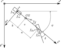
Figure 1: LT-CAR model. The figure show the quantities used to describe the model.

The body-frame of the car is attached at the rear contact point with $x$-$y$-$z$ axes oriented in a forward-right-down fashion. We let $\textbf{x}=[x,y,z]^{T}\in{\mathbb{R}}^{3}$ and $R\in SO(3)$ denote the position and orientation of the frame with respect to a fixed spatial-frame with $x$-$y$-$z$ axes oriented in a north-east-down fashion. $R$ maps vectors in the body frame to vectors in the spatial frame so that, for instance, the spatial angular velocity $\omega^{s}$ and the body angular velocity $\omega^{b}$ are related by $\omega^{s}=R\omega^{b}$ and $\omega^{b}=R^{T}\omega^{s}$. Similarly, $\textbf{x}^{s}=\textbf{x}+R\,\textbf{x}^{b}$ gives the spatial coordinates of a point on the body with body coordinates $\textbf{x}^{b}\in{\mathbb{R}}^{3}$. The orientation $R$ of the (unconstrained) rigid car model can be parameterized (using Roll-Pitch-Yaw parametrization) as follows

$$\small{R=R(\psi,\theta)=R_{z}(\psi)R_{y}(\theta)=\left[\begin{array}[]{ccc}c_{\psi}c_{\theta}&-s_{\psi}&c_{\psi}s_{\theta}\\ s_{\psi}c_{\theta}&c_{\psi}&s_{\psi}s_{\theta}\\ -s_{\theta}&0&c_{\theta}\\ \end{array}\right],}$$

where $\theta$ and $\psi$ are respectively the pitch and yaw angles (we use the notation $c_{\psi}=\cos(\psi)$, etc.). In the rest of the paper, for brevity, we use the notation $\phi=[\psi,\theta]^{T}$. The vector

$$q=[x,y,\psi,z,\theta]^{T}=[q_{r},q_{c}]^{T}$$

provides a valid set of generalized coordinates for dynamics calculations. The coordinates $q_{r}=[x,y,\psi]^{T}$ are the reduced unconstrained coordinates, while $q_{c}=[z,\theta]^{T}$ are the constrained ones.

II-A Tire models

We model the tire forces by using a suitable version of the Pacejka’s Magic Formula [27]. Before, we clarify our notation. We use a subscript “$f$” (“$r$”) for quantities of the front (rear) tire. When we want to give a generic expression that holds both for the front and the rear tire we just suppress the subscript. Thus, for example, we denote the generic normal tire force $f_{z}$, meaning that we are referring to $f_{fz}$ for the front tire and $f_{rz}$ for the rear one.

The rear and front forces tangent to the road plane, $f_{x}$ and $f_{y}$, depend on the normal force and on the longitudinal and lateral slips. The longitudinal slip $\kappa$ is the normalized difference between the angular velocity of the driven wheel $\omega_{w}$ and the angular velocity of the free-rolling $\omega_{0}=v_{cx}/r_{w}$, with $v_{cx}$ the contact point longitudinal velocity,

$$\kappa=\frac{\omega_{w}-\omega_{0}}{\omega_{0}}=-\frac{v_{cx}-r_{w}\omega_{w}}{v_{cx}}.$$

The lateral slip (or sideslip) $\beta$ is defined as $\tan{\beta}=v_{cy}/v_{cx}$, with $v_{cy}$ the lateral velocity. We assume that the rear and front forces tangent to the road plane, $f_{x}$ and $f_{y}$, depend linearly on the normal forces. Thus, the combined slip forces are

$$\begin{split}f_{x}=-f_{z}f_{x0}(\kappa)g_{x\beta}(k,\beta)=-f_{z}\mu_{x}(\kappa,\beta)\\ f_{y}=-f_{z}f_{y0}(\beta)g_{yk}(k,\beta)=-f_{z}\mu_{y}(\kappa,\beta),\end{split}$$

where the pure longitudinal slip $f_{x0}(\kappa)$, the pure lateral slip $f_{y0}(\beta)$ and the loss functions for combined slip $g_{x\beta}(\kappa,\beta)$ and $g_{yk}(\kappa,\beta)$ are defined in Appendix -A together with the values of the parameters used in the paper.

The front forces expressed in the body frame, $f_{fx}^{b}$ and $f_{fy}^{b}$, are obtained by rotating the forces in the tire frame according to the steer angle $\delta$, so that, e.g., $f_{fx}^{b}=f_{fx}c_{\delta}-f_{fy}s_{\delta}$. Substituting the above expressions for $f_{fx}$ and $f_{fy}$, we get

$$\begin{split}f_{fx}^{b}&=-f_{fz}\big{(}\mu_{fx}(\kappa_{f},\beta_{f})c_{\delta}-\mu_{fy}(\kappa_{f},\beta_{f})s_{\delta}\big{)}:=-f_{fz}\tilde{\mu}_{fx}(\kappa_{f},\beta_{f},\delta).\end{split}$$

In the rest of the paper, abusing notation, we will suppress the ‘tilde’ and use $\mu_{fx}(\kappa_{f},\beta_{f},\delta)$ to denote $\tilde{\mu}_{fx}(\kappa_{f},\beta_{f},\delta)$.

We assume to control the longitudinal slips $\kappa_{r}$ and $\kappa_{f}$. We want to point out that, depending on the analysis one can control the two slips independently or a combination of the two. For example, in the equilibrium manifold analysis and in the second trajectory exploration scenario we will set $\kappa_{f}=0$ and use only $\kappa_{r}$ as control input (rear-wheel drive). Thus, the control inputs of the car turn to be:

• $\kappa_{r}$ and $\kappa_{f}$, the rear and front longitudinal slips, and

• $\delta$, the front wheel steer angle.

Remark II.1 (Longitudinal slip as control input)

The use of the longitudinal slip as control input is present in the literature, e.g., [21] and [22]. This choice does not limit the applicability of our analysis. Indeed, wheel torques can be easily computed once a trajectory is computed. $\square$

Next, we introduce a simplified tire model that will be used to design approximate trajectories (trajectories of a simplified car model) characterized by contact forces that can not be generated by the Pacejka’s model. This simplified tire model, [4, 25, 28], relies on the following assumptions: (i) the longitudinal force is directly controlled, (ii) the relationship between the lateral force $f_{y}$ and the sideslip $\beta$ is linear, and (iii) the longitudinal and lateral forces, $f_{x}$ and $f_{y}$, are decoupled. We call the simplified car model obtained by using this tire approximation the Linear Tire LT-CAR (LT²-CAR). Figure 2 shows the plots of the longitudinal and lateral forces $f_{x}$ and $f_{y}$ for the Pacejka’s and linear tire models.

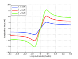
(a)

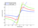
(b)

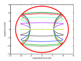
(c)

Figure 2: Pure longitudinal (a) and lateral (b) forces are plotted as function of respectively longitudinal and lateral slip for three values of the normal force. In (b) the simplified tire model (dashed line) is also shown. The longitudinal versus lateral force is plotted as function of the longitudinal slip for different values of the sideslip (c). The ellipse of maximum tire forces is shown in solid red.

Remark II.2 (Other tire models)

Tires are one of the key components of the vehicle and have an important impact on the performance. To capture the complex behavior of the tires several models have been developed in the literature [27], [29], [30]. We highlight that the LT-CAR model can be developed with any tire model (not necessarily the Pacejka’s one). $\square$

II-B Constrained Lagrangian dynamics

Next, we develop the constrained planar model of the rigid car and include load transfer. To describe the motion in the plane, we derive the equations of motion of the unconstrained system and explicitly incorporate the constraints (rather than choosing a subset of generalized coordinates). This allows us to have an explicit expression for the normal (constraint) forces.

We derive the dynamics of the unconstrained system via the Euler-Lagrange equations. To do this, we define the Lagrangian $\mathcal{L}$ as the difference between the kinetic and potential energies $\mathcal{L}(q,\dot{q})=T(q,\dot{q})-V(q)$. The equations of motion for the unconstrained system are given by the Euler-Lagrange equations

$$\frac{d}{dt}\frac{\partial\mathcal{L}}{\partial\dot{q}}^{T}-\frac{\partial\mathcal{L}}{\partial q}^{T}=U$$ (1)

where $U$ is the set of generalized forces. Exploiting the Euler-Lagrange equations, we get

$$M(q)\ddot{q}+C(q,\dot{q})+G(q)=U$$ (2)

with $M(q)$, $C(q,\dot{q})$ and $G(q)$ respectively the mass matrix, and the Coriolis and gravity vectors.

The longitudinal and lateral forces arising from the tire-road interactions at the front and rear contact points, $f=[f_{fx},f_{fy},f_{rx},f_{ry}]^{T}$, are converted into the generalized forces $U$ by using the principle of virtual work, $<\!f,v_{cp}^{b}\!>=<U,\dot{q}>$, where $v_{cp}^{b}=[v_{fx}^{b},v_{fy}^{b},v_{rx}^{b},v_{ry}^{b}]^{T}$ are the longitudinal and lateral velocities at the front and rear contact points. Computing the Jacobian matrix $J_{f}(\phi)$ mapping $\dot{q}$ to the front and rear contact point velocities expressed in the body frame, $v_{cp}^{b}=J_{f}(\phi)\dot{q}$, we get $<J_{f}(\phi)^{T}f,\dot{q}>=<U,\dot{q}>$, so that

$$U=J_{f}^{T}(\phi)f.$$

The front and rear contact points coordinates expressed in the body frame are $\textbf{x}_{f}^{b}=[a+b,0,0]^{T}$ and $\textbf{x}_{r}^{b}=[0,0,0]^{T}$. The coordinates in the spatial frame, respectively $\textbf{x}_{r}^{s}=[x_{r}^{s},y_{r}^{s},z_{r}^{s}]^{T}$ and $\textbf{x}_{f}^{s}=[x_{f}^{s},y_{f}^{s},z_{f}^{s}]^{T}$, are $\textbf{x}_{r}^{s}=\textbf{x}$ and $\textbf{x}_{f}^{s}=\textbf{x}+R\,\textbf{x}_{f}^{b}$, so that the velocities in the spatial frame are

$$v_{r}^{s}=\dot{\textbf{x}}\qquad\text{and}\qquad v_{f}^{s}=\dot{\textbf{x}}+R\,\omega^{b}\times\textbf{x}_{f}^{b}=\dot{\textbf{x}}-R\,\textbf{x}_{f}^{b}\times\omega^{b}=\dot{\textbf{x}}-R\,\hat{\textbf{x}}_{f}^{b}J_{\omega^{b}}(\phi)\dot{\phi},$$

where $\hat{\textbf{x}}_{f}^{b}$ is the skew-symmetric matrix associated to the vector $\textbf{x}_{f}^{b}$, while the velocities expressed in the body frame are

$$v_{r}^{b}=R^{T}\dot{\textbf{x}}=J_{v_{r}^{b}}(\phi)\dot{q}\,\qquad\text{and}\qquad v_{f}^{b}=R^{T}\dot{\textbf{x}}-\hat{\textbf{x}}_{f}^{b}J_{\omega^{b}}(\phi)\dot{\phi}=J_{v_{f}^{b}}(\phi)\dot{q}\,.$$

Thus, the Jacobian $J_{f}$ turns to be

$$J_{f}(\phi) =\small{\left[\begin{array}[]{c}J_{v_{fx}^{b}}\\ J_{v_{fy}^{b}}\\ J_{v_{rx}^{b}}\\ J_{v_{ry}^{b}}\end{array}\right]}=\small{\left[\begin{array}[]{ccccc}c_{\psi}c_{\theta}&s_{\psi}c_{\theta}&0&-s_{\theta}&0\\ -s_{\psi}&c_{\psi}&(a+b)c_{\theta}&0&0\\ c_{\psi}c_{\theta}&s_{\psi}c_{\theta}&0&-s_{\theta}&0\\ -s_{\psi}&c_{\psi}&0&0&0\\ \end{array}\right]}\,.$$

Next, we constrain the contact points to the road plane in order to compute the normal tire forces as reaction forces. We impose the constraint that the rear and front contact points have zero velocity along the $z$ axis. The velocity constraints are given by $\dot{z}_{r}=e_{3}^{T}R^{T}\dot{\textbf{x}}=J_{v^{b}_{rz}}(\phi)\dot{q}=0$, and $\dot{z}_{f}=e_{3}^{T}(R^{T}\dot{\textbf{x}}-\hat{\textbf{x}}_{f}^{b}J_{\omega^{b}}(\phi)\dot{\phi})=J_{v^{b}_{fz}}(\phi)\dot{q}=0$, where $e_{3}=[0,0,1]^{T}$, and $z_{r}$ ($z_{f}$) is the position of the rear (front) contact point expressed in the body frame. The front and rear constraints may be written in the form $A(q)\dot{q}=0$, where

$$\begin{split}A(q)\!=\!\begin{bmatrix}J_{v^{b}_{fz}}(\phi)\\ J_{v^{b}_{rz}}(\phi)\\ \end{bmatrix}=\!\begin{bmatrix}c_{\psi}s_{\theta}&s_{\psi}s_{\theta}&0&c_{\theta}&-(a+b)\\ c_{\psi}s_{\theta}&s_{\psi}s_{\theta}&0&c_{\theta}&0\\ \end{bmatrix}\!.\end{split}$$ (3)

From the principle of virtual work, we get the vector of constraint generalized forces, $U_{c}$, in terms of the front and rear normal contact point forces, $\lambda=[-f_{fz},~{}-f_{rz}]^{T}\in{\mathbb{R}}^{2}$, as $U_{c}=-A^{T}(q)\lambda$.

In the next proposition we show that, under the linear dependence of the contact point forces on the normal ones, the constrained system can be explicitly written as an unconstrained ordinary differential equation. Since the proof follows classical arguments from mechanics, we reported it in Appendix -B as a tutorial contribution.

Proposition II.3

Given the unconstrained car model with structure as in (2) and constraints in (3), the following holds true:

1. the dynamics of the constrained system can be written in terms of the unconstrained coordinates $q_{r}=[x,y,\psi]^{T}$ and the reaction forces $\lambda=[-f_{fz},~{}-f_{rz}]^{T}$ as

   $$\tilde{\mathcal{M}}(q_{r})\left[\begin{array}[]{c}\ddot{q}_{r}\\ \lambda\\ \end{array}\right]+\mathcal{C}(q_{r},\dot{q}_{r})+\mathcal{G}(q_{r})=\mathcal{U},$$ (4)

   where

   $$\tilde{\mathcal{M}}(q_{r})=\left[\begin{array}[]{cc}\mathcal{M}_{11}(q_{r})&0\\ \mathcal{M}_{21}(q_{r})&\mathcal{M}_{22}(q_{r})\\ \end{array}\right]=\small{\left[\begin{array}[]{ccc|cc}m&0&-mbs_{\psi}&0&0\\ 0&m&mbc_{\psi}&0&0\\ -mbs_{\psi}&mbc_{\psi}&I_{zz}+mb^{2}&0&0\\ \hline\cr 0&0&0&1&1\\ -mhc_{\psi}&-mhs_{\psi}&0&-(a+b)&0\end{array}\right]},$$

   $$\mathcal{C}(q_{r},\dot{q}_{r})=\left[\begin{array}[]{c}\mathcal{C}_{1}(q_{r},\dot{q}_{r})\\ \mathcal{C}_{2}(q_{r},\dot{q}_{r})\\ \end{array}\right]=\small{\left[\begin{array}[]{c}-mbc_{\psi}\dot{\psi}^{2}\\ -mbs_{\psi}\dot{\psi}^{2}\\ 0\\ \hline\cr 0\\ (I_{xz}+mhb)\dot{\psi}^{2}\end{array}\right]},\;\mathcal{G}(q_{r})=\left[\begin{array}[]{c}\mathcal{G}_{1}(q_{r})\\ \mathcal{G}_{2}(q_{r})\\ \end{array}\right]=\small{\left[\begin{array}[]{c}0\\ 0\\ 0\\ \hline\cr-mg\\ mgb\end{array}\right]},$$ (5)

   $$\small{\mathcal{U}=\left[\begin{array}[]{c}\mathcal{U}_{1}\\ \hline\cr 0\end{array}\right]=\left[\begin{array}[]{cccccc}c_{\psi}&-s_{\psi}&c_{\psi}&-s_{\psi}\\ s_{\psi}&c_{\psi}&s_{\psi}&c_{\psi}\\ 0&a+b&0&0\\ \hline\cr 0&0&0&0\\ 0&0&0&0\\ \end{array}\right]\left[\begin{array}[]{c}f_{fx}\\ f_{fy}\\ f_{rx}\\ f_{ry}\end{array}\right];}$$ (6)

2. the subsystem

   $$\mathcal{M}_{11}(q_{r})\ddot{q}_{r}+\mathcal{C}_{1}(q_{r},\dot{q}_{r})+\mathcal{G}_{1}(q_{r})=\mathcal{U}_{1}$$ (7)

   is a Lagrangian system obtained from a suitable reduced Lagrangian $\mathcal{L}_{r}(q_{r})$, with constraint forces $\lambda$ determined by

   $$\mathcal{M}_{21}(q_{r})\ddot{q}_{r}+\mathcal{M}_{22}(q_{r})\lambda+\mathcal{C}_{2}(q_{r},\dot{q}_{r})+\mathcal{G}_{2}(q_{r})=0;$$

3. under the assumption that the forces $f$ depend linearly on the reaction forces, i.e. $f=F\lambda$, the car dynamics turn to be

   $$\mathcal{M}(q_{r},\mu)\left[\begin{array}[]{c}\ddot{q}_{r}\\ \lambda\\ \end{array}\right]+\mathcal{C}(q_{r},\dot{q}_{r})+\mathcal{G}(q_{r})=0$$ (8)

   with

   $$\mathcal{M}(q_{r},\mu)=\left[\begin{array}[]{cc}\mathcal{M}_{11}(q_{r})&\mathcal{M}_{12}(q_{r},\mu)\\ \mathcal{M}_{21}(q_{r})&\mathcal{M}_{22}(q_{r})\\ \end{array}\right].$$

Remark II.4

Equation (8) can be exploited as

$$\begin{split}\ddot{q}_{r}&=\small{-(\mathcal{M}_{11}+\mathcal{M}_{12}\mathcal{M}_{22}^{-1}\mathcal{M}_{21})^{-1}}[\mathcal{C}_{1}+\mathcal{G}_{1}+\mathcal{M}_{12}\mathcal{M}_{22}^{-1}(\mathcal{C}_{2}+\mathcal{G}_{2})]\\ \lambda&=-\mathcal{M}^{-1}_{22}(\mathcal{C}_{2}+\mathcal{G}_{2}+\mathcal{M}_{21}\ddot{q}_{r}).\end{split}$$

From this expression it is clear that we have a dynamic model explicitly depending on the unconstrained coordinates $x$, $y$ and $\psi$ and an explicit expression for the reaction forces that can be used to calculate the normal loads for the tire forces. $\square$

II-C Model well-posedness and load transfer analysis

An important aspect to investigate is the well-posedness of the constrained model (8). Differently from the standard unconstrained equations of motion, as in (2), for which the mass matrix is always positive definite (and thus invertible), the invertibility of the matrix $\mathcal{M}(q_{r},\mu)$ depends on the model and tire parameters.

Proposition II.5

The LT-CAR model is well-posed if the following inequalities are satisfied

$$\begin{split}\mu_{rx}<\frac{I_{xz}\dot{\psi}^{2}}{mgh}+\frac{b}{h}\;\;\text{and}\;\;\mu_{fx}>\frac{I_{xz}\dot{\psi}^{2}}{mgh}-\frac{a}{h}.\end{split}$$ (9)

Proof:

By means of simple operations on the $\mathcal{M}$ matrix, we can compute the normal forces

$$f_{fz}=\frac{mgb-mgh\mu_{rx}+I_{xz}\dot{\psi}^{2}}{h\left(\mu_{rx}-\mu_{fx}\right)-(a+b)}\,,\qquad f_{rz}=\frac{mga+mgh\mu_{fx}-I_{xz}\dot{\psi}^{2}}{h(\mu_{rx}-\mu_{fx})-(a+b)}\,.$$ (10)

In order for the model to be valid, both the two reaction forces, $f_{fz}$ and $f_{rz}$, need to be negative. Indeed, the ground is a unilateral constraint and, therefore, cannot generate a positive reaction force. Clearly, if the two conditions in (9) are satisfied, the denominator of the two reaction forces is negative and both the two nominators are positive, thus concluding the proof. ∎

Remark II.6

From the combined slip Pacejka’s formulas, $\mu_{rx}$ and $\mu_{fx}$ are bounded by

$$|\mu_{rx}| =|f_{rx0}(\kappa_{r})g_{rx\beta}(\kappa_{r},\beta_{r})|\leq d_{x}^{r}$$

$$|\mu_{fx}| =|c_{\delta}f_{fx0}(\kappa_{f})g_{fx\beta}(\kappa_{f},\beta_{f})-s_{\delta}f_{fy0}(\beta_{f})g_{fx\beta}(\kappa_{f},\beta_{f})|\leq(d_{x}^{f}+d_{y}^{f}).$$

Thus, for the data provided in Appendix -A, the conditions of Proposition II.5 are always satisfied for “reasonable” values of $\dot{\psi}$ (e.g., for $|\dot{\psi}|<2\pi$ rad/s). $\square$

Equations (10) show the influence of the front and rear longitudinal force coefficients on the load transfer. A sharp acceleration, due to a high (positive) value of $\mu_{rx}$, increases the load on the rear wheel while reducing the load on the front. Similarly, a hard braking, mainly due to a high (negative) value of $\mu_{fx}$, increases the front normal load while reducing the normal load on the rear. In particular, if $\mu_{rx}=\frac{I_{xz}\dot{\psi}^{2}+mgb}{mgh}$, then the front wheel leaves the ground, thereby producing a “wheelie”; if $\mu_{fx}=\frac{I_{xz}\dot{\psi}^{2}-mga}{mgh}$, then the rear wheel leaves the ground, thereby producing a “stoppie”. In Figure 3, we provide a graphical representation of the model validity region.

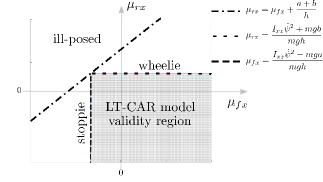
Figure 3: Well-posedness interpretation of the model. LT-CAR model validity region: the wheelie and stoppie conditions are avoided, i.e. $-f_{fz}>0$ and $-f_{rz}>0$.

II-D Dynamics in the body frame

We provide the dynamics in the body frame with two different set of coordinates. These dynamics will be helpful in the characterization of the equilibrium manifold and in the exploration strategy. Indeed, expressing the dynamics in the body frame, allows us to decouple them from the kinematics and, thus, write a reduced model which includes only velocities and accelerations.

Since the dynamics do not depend on the positions $x$ and $y$, and the orientation $\psi$, we can work directly with the longitudinal velocity $v_{x}$ and the lateral velocity $v_{y}$. To do this, note that

$$\left[\begin{array}[]{c}\ddot{x}\\ \ddot{y}\\ \end{array}\right]=R_{z}(\psi)\left[\begin{array}[]{c}\dot{v}_{x}-v_{y}\dot{\psi}\\ \dot{v}_{y}+v_{x}\dot{\psi}\\ \end{array}\right].$$ (11)

Thus, we get the equations in (12).

One more version of the dynamics is obtained by choosing as states the vehicle speed $v$ and the vehicle sideslip angle $\beta$, where $\tan\beta=v_{y}/v_{x}$. This change of coordinates is helpful to calculate the equilibrium manifold in the next section. In this case, denoting $\chi=\psi+\beta$ the orientation of the velocity with respect to the spatial frame, we have

$$\left[\begin{array}[]{c}\ddot{x}\\ \ddot{y}\\ \end{array}\right]=R_{z}(\chi)\left[\begin{array}[]{c}\dot{v}\\ v\dot{\chi}\\ \end{array}\right]=R_{z}(\psi)R_{z}(\beta)\left[\begin{array}[]{c}\dot{v}\\ v\dot{\chi}\\ \end{array}\right],$$

where $\dot{v}$ and $v\dot{\chi}$ are the longitudinal and lateral accelerations, respectively. Finally, considering the relation (11) we have

$$\left[\begin{array}[]{c}\dot{v}\\ v\dot{\beta}\\ \end{array}\right]=R_{z}(\beta)^{T}\left[\begin{array}[]{c}\dot{v}_{x}-v_{y}\dot{\psi}\\ \dot{v}_{y}+v_{x}\dot{\psi}\\ \end{array}\right]-\left[\begin{array}[]{c}0\\ v\dot{\psi}\\ \end{array}\right],$$

so that the equations of motion are the one given in (13).

We have a family of car models, (12) and (13), that provide different insights depending on the features to investigate. The model (12) is used to explore the dynamics of the car vehicle; the models (12) and (13) are used to solve the equilibrium manifold (under usual driving conditions, it is natural to specify $v$ and $\beta$).

$$\footnotesize{\begin{bmatrix}m&0&0&\mu_{fx}&\mu_{rx}\\ 0&m&mb&\mu_{fy}&\mu_{ry}\\ 0&mb&(I_{zz}+mb^{2})&(a+b)\mu_{fy}&0\\ 0&0&0&-1&-1\\ -mh&0&0&a+b&0\\ \end{bmatrix}\left[\begin{array}[]{c}\dot{v}_{x}\\ \dot{v}_{y}\\ \ddot{\psi}\\ f_{fz}\\ f_{rz}\\ \end{array}\right]+\begin{bmatrix}-mb\dot{\psi}^{2}-mv_{y}\dot{\psi}\\ mv_{x}\dot{\psi}\\ mbv_{x}\dot{\psi}\\ 0\\ (I_{xz}+mhb)\dot{\psi}^{2}+mhv_{y}\dot{\psi}\\ \end{bmatrix}+\begin{bmatrix}0\\ 0\\ 0\\ -mg\\ mgb\\ \end{bmatrix}=\begin{bmatrix}0\\ 0\\ 0\\ 0\\ 0\\ \end{bmatrix}}$$ (12)

$$\footnotesize{\begin{bmatrix}mc_{\beta}&-mvs_{\beta}&0&\mu_{fx}&\mu_{rx}\\ ms_{\beta}&mvc_{\beta}&mb&\mu_{fy}&\mu_{ry}\\ mbs_{\beta}&mbvc_{\beta}&(I_{zz}+mb^{2})&(a+b)\mu_{fy}&0\\ 0&0&0&-1&-1\\ -mhc_{\beta}&mhvs_{\beta}&0&a+b&0\\ \end{bmatrix}\!\left[\begin{array}[]{c}\dot{v}\\ \dot{\beta}\\ \ddot{\psi}\\ f_{fz}\\ f_{rz}\\ \end{array}\right]\!+\!\begin{bmatrix}-mv\dot{\psi}s_{\beta}-mb\dot{\psi}^{2}\\ -mv\dot{\psi}c_{\beta}\\ mbv\dot{\psi}c_{\beta}\\ 0\\ (I_{xz}+mhb)\dot{\psi}^{2}+mhv\dot{\psi}s_{\beta}\\ \end{bmatrix}\!+\!\begin{bmatrix}0\\ 0\\ 0\\ -mg\\ mgb\\ \end{bmatrix}\!=\!\begin{bmatrix}0\\ 0\\ 0\\ 0\\ 0\\ \end{bmatrix}}$$ (13)

Remark II.7 (Model development and existing literature)

The proposed LT-CAR model development differs form the one proposed in [9] as follows. First, we provide a detailed derivation of the model based on the Lagrangian approach. This derivation allows us to exploit an interesting structure of the proposed car vehicle. Second, we consider the off-diagonal inertia term $I_{xz}$, see the Coriolis term in (12) and (13), which becomes significant in studying both cornering equilibria and aggressive maneuvers. Third and final, we analyze the region of model validity in terms of the vehicle (geometric and tire) parameters. $\square$

III Equilibrium Manifold

In this section we analyze the equilibrium manifold of the car model, i.e. the set of trajectories that can be performed by use of constant inputs. Searching for “constant” trajectories requires the solution of a set of nonlinear equations expressing the fact that all accelerations must be set to zero. To define an equilibrium trajectory, we refer to the car model in the form (13). The equilibria are obtained by enforcing

$$(\dot{v},\dot{\beta},\ddot{\psi})=(0,0,0).$$ (14)

The corresponding trajectory of the full car model (including position and orientation) is a circular path at constant speed $v$, yaw rate $\dot{\psi}$ and vehicle sideslip angle $\beta$. Since $\dot{\beta}=0$, the lateral acceleration is given by $a_{lat}=v\dot{\psi}$, and expressing the accelerations in the body frame as follows,

$$\left[\begin{array}[]{c}a_{x}\\ a_{y}\\ \end{array}\right]=\left[\begin{array}[]{c}\dot{v}_{x}-v_{y}\dot{\psi}\\ \dot{v}_{y}+v_{x}\dot{\psi}\\ \end{array}\right]=R_{z}(\beta)\left[\begin{array}[]{c}\dot{v}\\ v\dot{\chi}\\ \end{array}\right]$$

we have

$$a_{x}=-a_{lat}\sin{\beta}\,,\quad a_{y}=a_{lat}\cos{\beta}\,,\quad\dot{\psi}=a_{lat}/v.$$

Now, referring to the dynamic model (13), we set the constraints (14) and we get two equations from the load transfer in equilibrium condition

$$\begin{split}-f_{fz}&=mg\frac{b}{a+b}+\frac{(I_{xz}+mhb)(\frac{a_{lat}}{v})^{2}+a_{lat}mh\sin\beta}{a+b}\\ -f_{rz}&=mg\frac{a}{a+b}-\frac{(I_{xz}+mhb)(\frac{a_{lat}}{v})^{2}+a_{lat}mh\sin\beta}{a+b}\end{split}$$ (15)

and the following three equations from the system dynamics:

$$\begin{split}ma_{x}-mb\dot{\psi}^{2}+\mu_{fx}f_{fz}+\mu_{rx}f_{rz}&=0\\ ma_{y}+\mu_{fy}f_{fz}+\mu_{ry}f_{rz}&=0\\ mba_{y}+(a+b)\mu_{fy}f_{fz}&=0.\\ \end{split}$$ (16)

For the clarity of presentation, we perform the equilibrium manifold computation by using only the rear slip $\kappa_{r}$ as control input (and setting the longitudinal one, $\kappa_{f}$, to zero). Substituting the expression of the normal forces (15) into equations (16), we obtain a nonlinear system of three equations in five unknowns ($v$, $a_{lat}$, $\beta$, $\delta$ and $\kappa_{r}$), so that the equilibrium manifold is a two-dimensional surface. We parameterize the equilibrium manifold in terms of the car speed and lateral acceleration ($v$ and $a_{lat}$), so that the slip angle, steer angle and longitudinal slip ($\beta$, $\delta$ and $\kappa_{r}$) are obtained by solving the nonlinear equations in (16).

We solve the nonlinear system by using a predictor corrector continuation method, as described in [24], relying on the continuity of the equilibria with respect to the equilibrium manifold parameters $v$ and $a_{lat}$. Next, we describe the predictor corrector continuation method applied to the equilibrium manifold of our car model. We fix the velocity $v$ and explore a one-dimensional slice of the manifold. First, we provide a useful lemma from [24].

Lemma III.1 (Lemma 2.1.3, [24])

Let $\ell:{\mathbb{R}}^{n+1}\rightarrow{\mathbb{R}}^{n}$ be a smooth nonlinear function such that $\ell(\eta_{0})=0$ for some $\eta_{0}\in{\mathbb{R}}^{n+1}$ and let the Jacobian matrix $D\ell(\eta_{0})\in{\mathbb{R}}^{n\times(n+1)}$ have maximum rank. Then, there exists a smooth curve $s\in[0,s_{1})\mapsto c(s)\in{\mathbb{R}}^{n+1}$, parametrized with respect to arclength $s$, for some open interval $[0,s_{1})$ such that for all $s\in[0,s_{1})$: i) $c(0)=\eta_{0}$, ii) $\ell(c(s))=0$, iii) $rank(D\ell(c(s)))=n$, and iv) $\dot{c}(s)\neq 0$. $\square$

Let $\eta=[a_{lat},\beta,\delta,\kappa_{r}]^{T}$ and let $\ell(\eta)=0$ be the nonlinear system in (16), with $\ell:{\mathbb{R}}^{4}\rightarrow{\mathbb{R}}^{3}$. The following proposition shows that there exists a one dimensional manifold of solution points.

Proposition III.2 (Equilibrium manifold well posedness)

Given the nonlinear system in (16), the following holds true:

1. there exists a smooth curve $s\in[0,s_{1})\mapsto c(s)\in{\mathbb{R}}^{4}$, for some $s_{1}>0$, such that $\ell(c(s))=0$ for all $s\in[0,s_{1})$;

2. $c(s)$ is the local solution of

   $$\begin{split}\dot{\eta}=v^{\top}(\eta)\qquad\eta(0)=\eta_{0},\end{split}$$ (17)

   where $v^{\top}(\eta)$ is the tangent vector induced by $D\ell(\eta)$.

Proof:

To prove statement (i), we use Lemma III.1. The nonlinear function $\ell$ contains sums and products of trigonometric and power functions, thus it is smooth. Using the expression of the combined slip forces introduced in Section II-A, for $\eta_{0}=[0,0,0,0]^{T}$ we have $\mu=0$, so that $\ell(\eta_{0})=0$. Moreover, by explicit calculation, the Jacobian matrix at $\eta_{0}$ has rank three.

To prove statement (ii), we differentiate $\ell(c(s))=0$ with respect to the arc-length $s$. The tangent $\dot{c}(s)$ satisfies $D\ell(c(s))\dot{c}(s)=0,\,\,\,\|\dot{c}(s)\|=1\;\;\forall s\in[0,s_{1})$. Hence $\dot{c}(s)$ spans the one-dimensional kernel $ker(D\ell(c(s)))$, or equivalently, $\dot{c}(s)$ is orthogonal to all rows of $D\ell(c(s))$. In other words, the unique vector $\dot{c}(s)$ is the tangent vector induced by $D\ell(c(s))$, $v^{\top}(\eta)$. Using the Implicit Function Theorem, e.g., [31], the tangent vector $v^{\top}(\eta)$ depends smoothly on $D\ell(c(s))$. Thus, $c$ is the solution curve of the initial value problem in (17), which concludes the proof. ∎

In order to numerically trace the curve $c$ efficiently, we use a predictor-corrector method. The main idea is to generate a sequence of points along the curve $\eta_{i}$, $i=1,2,\ldots$, that satisfy a given tolerance, say $\|\ell(\eta_{i})\|\leq\nu$ for some $\nu>0$. So, for $\nu>0$ sufficiently small, there is a unique parameter value $s_{i}$ such that the point $c(s_{i})$ on the curve is nearest to $\eta_{i}$ in Euclidean norm. To describe how points $\eta_{i}$ along the curve $c$ are generated, suppose that a point $\eta_{i}\in{\mathbb{R}}^{4}$ satisfies the chosen tolerance (i.e. $\|\ell(\eta_{i})\|\leq\nu$). If $\eta_{i}$ is a regular point of $\ell$, then there exists a unique solution curve $c_{i}:[0,s_{1})\rightarrow{\mathbb{R}}^{4}$ which satisfies the initial value problem (17) with initial condition $\eta(0)=\eta_{i}$.

To obtain a new point $\eta_{i+1}$ along $c$, we make a predictor step as a simple numerical integration step for the initial value problem. We use an Euler predictor: $\alpha_{i+1}=\eta_{i}+\epsilon\,v^{\top}(\eta)$, where $\epsilon>0$ represents a suitable stepsize. The corrector step computes the point $\omega_{i+1}$ on $c$ which is nearest to $\alpha_{i+1}$. The point $\omega_{i+1}$ is found by solving the optimization problem

$$\|\omega_{i+1}-\alpha_{i+1}\|=\min_{\ell(\omega)=0}\|\omega-\alpha_{i+1}\|\,.$$ (18)

If the stepsize $\epsilon$ is sufficiently small (so that the predictor point $\alpha_{i+1}$ is sufficiently close to the curve $c$) the minimization problem has a unique solution $\omega_{i+1}$. We compute $\omega_{i+1}$ by using a Newton-like method. The Newton point $\mathcal{N}(\alpha)$ for approximating the solution of (18) is given by $\mathcal{N}(\alpha)=\alpha-D\ell(\alpha)^{\dagger}\ell(\alpha)$.

The predictor-corrector continuation method used in the paper thus consists of repeatedly performing these predictor and corrector steps as shown in the pseudo-code below.

Algorithm 1 Predictor-corrector continuation method

0:  initial equilibrium condition $\eta_{0}$ such that $\ell(\eta_{0})=0$

  for $i=0,1,2\ldots$ do

     set the initial steplength $\epsilon_{i}=\overline{\epsilon}$;

     loop

        get predictor step: $\alpha_{i+1}=\eta_{i}+\epsilon_{i}\,v^{\top}(\eta)$;

        search corrector term:           $\omega_{i+1}=\alpha_{i+1}-D\ell(\alpha_{i+1})^{\dagger}\ell(\alpha_{i+1})$;           $\alpha_{i+1}=\omega_{i+1}$;

        if convergence then break;

        else update step-length $\epsilon_{i+1}=\frac{\epsilon_{i}}{2}$;end if

     end loop

     $\eta_{i+1}=\omega_{i+1}$;

  end for

We compute and compare the equilibrium manifold for the car model with and without load transfer (i.e. LT-CAR and bicycle model). The model parameters are the one of a sports car with rear-wheel drive transmissions given in Appendix -A.

​ ​​​​​ ​​​​​ ​

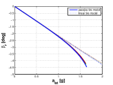
(a)

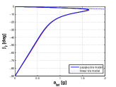
(b)

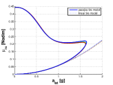
(c)

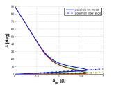
(d)

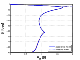
(e)

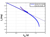
(f)

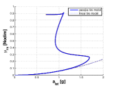
(g)

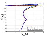
(h)

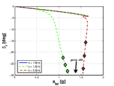
(a)

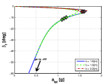
(b)

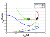
(c)

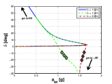
(d)

Figure 5: Equilibrium manifold for a rear-wheel drive sports car for different positions of the center of mass. Specifically: rear sideslip, front sideslip, longitudinal force coefficient and steer angle for $v=30$ m/s, $b=(1.6,1.9,2.1)$ m and $a+b=2.45$ m. In (d) the red and green diamond markers show three equilibrium points with steer angle opposite to the direction of the turn (counter-steering).

​ ​​​​​ ​​​​​ ​

Figure 4: Equilibrium manifold for a rear-wheel drive sports car with longitudinal load transfer in (a)-(d), and without load transfer in (e)-(h). Specifically: rear and front sideslip, longitudinal force coefficient, and steer angle for $v=(20,30,40)$ m/s. Dot lines in (a)-(b)-(c) and (e)-(f)-(g) are the equilibria with linear tire model. The dash-dot line in (d) and (h) is the Ackerman steer angle.

​ ​​​​​ ​ ​​​​​

Some slices of the equilibrium manifold are shown in Figure 5. The plots are given only for positive values of the lateral acceleration due to the symmetry of the equilibrium manifold. Indeed, the rear and front sideslip, and the steer angle are symmetric functions of $a_{lat}$, while the longitudinal force coefficient is antisymmetric.

For low longitudinal and lateral slips a first class of equilibria appears. These equilibria are close to the ones with the linear tire approximation (the solid lines in Figures 5 are close to the dot lines). Indeed, for low slips ($\beta_{r},\beta_{f}<5$ deg and $\kappa_{r}<0.05$) the tires work within their linear region as appears in Figures 2a and 2b. To characterize the vehicle behavior in this region, we can use, [5], the understeer gradient

$$K_{us}(a_{lat};v)=\frac{\partial\delta(a_{lat};v)}{\partial a_{lat}}-K_{a},$$

where $K_{a}=\frac{a+b}{v^{2}}$ is called Ackerman steer angle gradient. The vehicle is said to be understeering if $K_{us}>0$, neutral if $K_{us}=0$ and oversteering if $K_{us}<0$. From a graphical point of view, the understeering behavior can be measured by looking at how much the curve $a_{lat}\mapsto\delta(a_{lat};v)$, for fixed $v$, departs from the line $a_{lat}\mapsto K_{a}a_{lat}$. As shown in Figure 4d and 4h, the steer angle gradient is slightly negative, which suggests an oversteering behavior $K_{us}<0$. It is worth noting that if the relationship between $a_{lat}$ and $\beta$ ($=\beta_{r}$) is approximately linear, then the load transfer is approximately quadratic as a function of $a_{lat}$ by (15). This is in fact what occurs in this case (see Figure 4a), so that $-f_{rz}$ increases approximately quadratically with $a_{lat}$ (with $-f_{fz}$ decreasing by the same amount). That is, with increased lateral acceleration, we see that the rear tire(s) becomes more effective (due to increased loading) and the front becomes less effective.

For high values of the longitudinal and lateral slips the equilibrium manifolds depart from their linear-tire approximation. Indeed, the linear tires, without force saturation, can generate a lateral force for a wider range of lateral acceleration. We observe a significantly different structure of the equilibrium manifold for the two models, which gives a first evidence of the importance of taking into account the load transfer phenomenon. Specifically, since the available tire force is limited for the LT-CAR model, the achievable lateral acceleration is also limited. This limit occurs as a smooth turning of the equilibrium manifold as seen in, e.g., Figures 4b and  4c, and the manifold can be continued with steering going all the way to $90$[deg] at which point the front tire(s) is just pushing with no lateral force. The steady-state behavior of the LT-CAR is clear: for a given $v$ and $a_{lat}$, the required $\beta$ is close to that predicted by the linear tire model while there are two solutions (except at the maximum value of $a_{lat}$) for the steering angle providing rather different values of $\beta_{f}$ and $\kappa_{r}$. This straightforward behavior of $\beta$ seems to be related to the fact that the rear tire(s) becomes more effective as $a_{lat}$ is increased. In contrast, for the bicycle model (i.e., without load transfer) the front tire(s) retains a higher loading and its equilibrium manifold shows that it is the front sideslip $\beta_{f}$ that keeps a small angle (so that the front wheel is nearly aligned with the direction of travel) while the rear sideslip is allowed to be quite large, see Figures 4e and 4f. Topologically, the equilibrium manifolds of the system with and without load transfer are strikingly different. Clearly, the load transfer is the responsible of this difference due to its modulating action on the ground forces.

The predictor-corrector continuation method can be also used to perform a sensitivity analysis of the equilibrium manifold with respect to the car parameters (as, e.g., mass, moment of inertia, center of mass position). In Figure 4d we highlight the results obtained when varying the center of mass position along the body longitudinal axis. By setting the sports car inertial parameters, we compute the manifold varying the value of $a$ and $b$ with constant wheelbase $a+b=2.45$ m. When the center of mass is moved over the half wheelbase toward the front axle, the manifold has a significantly different structure (green and red lines). In particular, the equilibria at highest rear lateral and longitudinal slips, highlighted with the red diamond markers, are achieved with steer angle opposite to the direction of the turn (counter-steering). This car set up resembles the one of rally cars which, indeed, take advantage of the counter-steering behavior in performing aggressive turns. The significant change of the equilibrium manifold with respect to the position of the center of mass suggests that the equilibrium manifold sensitivity analysis can be used as a design tool to optimize the car performance. Thus, a deep investigation of these and other parameters on the shape of the equilibrium manifold (and hence on the nonlinear system behavior) would be an interesting area of research.

IV Nonlinear optimal control based trajectory exploration

In this section we describe the optimal control based strategies used to explore the dynamics of the car vehicle and provide numerical computations showing their effectiveness.

IV-A Exploration strategy based on least-square optimization

Complex dynamic interactions make the development of maneuvers highly nontrivial. To this end, we use nonlinear least squares trajectory optimization to explore system trajectories. That is, we consider the optimal control problem

$$\begin{split}\min&\;\;\frac{1}{2}\int_{0}^{T}\|\textrm{x}(\tau)-\textrm{x}_{d}(\tau)\|_{Q}^{2}+\|\textrm{u}(\tau)-\textrm{u}_{d}(\tau)\|_{R}^{2}d\tau+\frac{1}{2}\|\textrm{x}(T)-\textrm{x}_{d}(T)\|_{P_{1}}^{2}\\ \text{subj. to}&\;\;\dot{\textrm{x}}(t)=f(\textrm{x}(t),\textrm{u}(t))\qquad\textrm{x}(0)=\textrm{x}_{0},\end{split}$$ (19)

where $Q$, $R$ and $P_{1}$ are positive definite weighting matrices, for $z\in{\mathbb{R}}^{n}$ and $W\in{\mathbb{R}}^{n\times n}$ $\|z\|_{W}^{2}=z^{T}Wz$, and $(\textrm{x}_{d}(\cdot),\textrm{u}_{d}(\cdot))$ is a desired curve.

We propose an optimal control based strategy to solve the optimal control problem (19) and compute aggressive vehicle trajectories. The strategy is based on the projection operator Newton method, [26], see Appendix -D. We want to stress that the projection operator Newton method, as any other a descent method, guarantees the convergence to a local minimum of the optimal control problem in (19). Thus, a naive application of this method (or any other available optimal control solver) may let the algorithm converge to a (local minimum) trajectory that is too far from the desired curve and does not contain useful information on the vehicle capabilities. In order to deal with this issue, we develop an exploration strategy based on the following features: (i) choose a desired (state-input) curve that well describes the desired behavior of the vehicle, (ii) embed the original optimal control problem into a class of problems parametrized by the desired curve, and (iii) design a continuation strategy to morph the desired curve from an initial nonaggressive curve up to the target one.

IV-A1 Desired Curve design

First, we describe how to choose the desired curve. The path and the velocity profile to follow on that path, are usually driven by the exploration objective. Thus, the positions $x_{d}(t)$ and $y_{d}(t)$ and the velocity $v_{d}(t)$, with $t\in[0,T]$, of the desired curve are assigned. For example, in the next sections we describe two maneuvers where we want to understand the vehicle capabilities in following respectively a chicane at “maximum speed” and a real testing track at constant speed.

How to choose the other portion of the desired curve (i.e. the remaining states and the inputs) strongly affects the exploration process. In order to choose this portion of the desired curve, we use a quasi trajectory that, with some abuse of notation, we call quasi-static trajectory.

Given $x_{d}(t)$, $y_{d}(t)$, $v_{d}(t)$, and the curvature $\sigma_{d}(t)$, $t\in[0,T]$, for each $t\in[0,T]$, we impose the equilibrium conditions (14) for the desired velocity and path curvature at time $t$. That is, posing $v_{qs}(t)=v_{d}(t)$ and $\dot{\psi}_{qs}(t)=v_{d}(t)\sigma_{d}(t)$, we compute the corresponding equilibrium value for the sideslip angle, $\beta_{qs}(t)$, the yaw rate, $\dot{\psi}_{qs}(t)$, and the yaw angle, $\psi_{qs}(t)$, together with the steer angle, $\delta_{qs}(t)$, and the rear and front longitudinal slips, $\kappa_{r_{qs}}(t)$ and $\kappa_{f_{qs}}(t)$, by solving the nonlinear equations (16). Thus, the quasi-static trajectory $(\textrm{x}_{qs}(t),\textrm{u}_{qs}(t))$, $t\in[0,T]$, is given by

$$\textrm{x}_{qs}(t)= [x_{d}(t),\,y_{d}(t),\,\psi_{qs}(t),\,v_{d}(t),\,\beta_{qs}(t),\,v_{d}(t)\sigma_{d}(t)]^{T}\,,$$

$$\textrm{u}_{qs}(t)= [\delta_{qs}(t),\,\kappa_{r_{qs}}(t),\kappa_{f_{qs}}(t)]^{T}\,.$$

Remark IV.1

We stress that the quasi-static trajectory is not an LT-CAR trajectory since it does not satisfy the dynamics. However, experience shows that, for low values of the (longitudinal and lateral) accelerations, the quasi-static trajectory is close to the trajectory manifold. $\square$

The above considerations suggest that the quasi-static trajectory represents a reasonable guess of the system trajectory on a desired track for a given velocity profile. Thus, when only the desired position and velocity curves are available, we set the desired curve as the quasi-static trajectory, i.e. $\xi_{d}=(\textrm{x}_{qs}(\cdot),\textrm{u}_{qs}(\cdot))$. In doing this choice we remember that the positions and velocity profiles are the ones we really want to track, whereas the other state profiles are just a guess. Thus, we will weight the first much more than the latter.

Remark IV.2

Since we are interested in exploring “limit” vehicle capabilities, most of the times, as it happens in real prototype tests, we will study aggressive maneuvers characterized by high levels of lateral acceleration. Thus, it can happen that a quasi-static trajectory can not be found (we are out of the equilibrium manifold). If this is the case, we generate the desired curve by using the linear tires car model, LT²-CAR, discussed in Section II-A, so that higher lateral accelerations can be achieved. In this way we can compute the quasi-static trajectory, and thus the desired curve, for more aggressive path and velocity profiles. $\square$

IV-A2 Initial trajectory and optimal control embedding

With the desired curve in hand we still have the issue of choosing the initial trajectory to apply the projection operator Newton method. To design the initial trajectory, we could choose an equilibrium trajectory (e.g. a constant velocity on a straight line). However, such naive initial trajectory could lead to a local minimum that is significantly far from the desired behavior or cause a relatively high number of iterations. From the considerations in Remark IV.1, we know that a quasi-static trajectory obtained by a velocity profile that is not “too aggressive” is reasonably close to the trajectory manifold.

These observations motivate and inspire the development of an embedding and continuation strategy. We parametrize the optimal control problem in (19) with respect to the desired curve. Namely, we design a family of desired curves that continuously morph a quasi-static trajectory with a “non-aggressive” velocity profile into the actual desired (quasi-static) curve.

IV-A3 Continuation Update rule

We start with a non-aggressive desired curve, $\xi^{1}_{d}=(\textrm{x}^{1}_{d}(\cdot),\textrm{u}^{1}_{d}(\cdot))$, and choose as initial trajectory, $\xi^{1}_{0}$, the projection of the desired curve, $\xi^{1}_{0}=\mathcal{P}(\xi^{1}_{d})$. That is, we implement equation (22) with $(\alpha(\cdot),\mu(\cdot))=(\textrm{x}^{1}_{d}(\cdot),\textrm{u}^{1}_{d}(\cdot))$. Then, we update the temporary desired curve, $\xi^{i}_{d}$, with the new curve in the family, $\xi^{i+1}_{d}$, (characterized by a more aggressive velocity profile on the same track) and use as initial trajectory for the new problem the optimal trajectory at the previous step. The procedure ends when an optimal trajectory is computed for the optimal control problem where the temporary desired curve equals the actual one. Next, we give a pseudo code description of the exploration strategy. We denote PO_Newt$(\xi_{i},\xi_{d})$ the local minimum trajectory obtained by implementing the projection operator Newton method presented in Appendix -D for a given desired curve $\xi_{d}$ and initial trajectory $\xi_{i}$.

Algorithm 2 Exploration strategy

0:  desired path and velocity $x_{d}(\cdot)$, $y_{d}(\cdot)$ and $v_{d}(\cdot)$

  compute: desired curve $\xi_{d}=(\textrm{x}_{qs}(\cdot),\textrm{u}_{qs}(\cdot))$;design: $\xi_{d}^{i}$, $i\in\{1,\ldots,n\}$, s.t. $\mathcal{P}(\xi_{d}^{1})\simeq\xi_{d}^{1}$ and $\xi_{d}^{n}=\xi_{d}$;compute: initial trajectory $\xi_{0}^{1}=\mathcal{P}(\xi_{d}^{1})$.

  for $i=1,\ldots,n$ do

     compute: $\xi_{opt}^{i}$ = PO_Newt($\xi_{0}^{i}$, $\xi_{d}^{i}$);

     set: $\xi_{0}^{i+1}=\xi_{opt}^{i}$;

  end for

  $\xi_{opt}=\xi_{opt}^{n}$.

IV-B Aggressive maneuver on a chicane and model validation

As first computation scenario we perform an aggressive maneuver by using a Computer Aided Engineering (CAE) tool for virtual prototyping to generate the desired curve. CAE tools for virtual prototyping allow car designers to create a full vehicle model and perform functional tests, without realizing a physical prototype, with a very high level of reliability. As CAE tool, we use Adams/Car developed by MSC.Software. Adams is one of the most used multibody dynamics tools in the automotive industry.

The objective of this computation scenario is twofold: (i) we show the effectiveness of the exploration strategy in finding an LT-CAR trajectory close to the desired curve, and (ii) we validate the LT-CAR model by showing that the desired curve, which is a trajectory of the full Adams model, is in fact “almost” a trajectory of the LT-CAR model.

The desired curve is obtained as follows. We set as desired path the chicane depicted in Figure 6a. To obtain the desired velocity profile, we set the initial velocity to $150$ km/h ($41.67$ m/s), and invoke an Adams routine that generates a velocity profile to drive the vehicle on the given path at maximum speed under a maximum acceleration (a${}_{\texttt{max}}$). The remaining desired state curves are obtained by means of an Adams closed loop controller that drives the (Adams) vehicle on the given path with the given velocity profile. The desired inputs are set to zero since they do not have an immediate correspondence with the inputs of the Adams vehicle. They are weighted lightly, thus giving the optimization the necessary freedom to track the states. With this desired trajectory in hands, to “run” the exploration strategy, we need to define the initial trajectory and the continuation update rule for the desired trajectory morphing.

The exploration strategy for this maneuver is as follows. Initially, we limit the maximum acceleration parameter to $50\%$ of the desired one (a${}_{\texttt{max}}$₀ $=$ $50\%$ a${}_{\texttt{max}}$). This gives a trajectory that can be easily projected to the LT-CAR model to get a suitable initial trajectory. Then, we increase the vehicle capabilities of a $10\%$ acceleration step-size until the desired maximum acceleration is reached. For each intermediate step, we set the Adams trajectory as temporary desired trajectory and the optimal trajectory at the previous step as initial trajectory. A pseudo code of the strategy is given in the following table.

Algorithm 3 Exploration strategy for the chicane maneuver

  Run: Adams/Car with path = “chicane”      compute: velocity profile with a${}_{\texttt{max}}$₀ = $50\%$ a${}_{\texttt{max}}$      run: closed-loop driver to get $\xi_{d}^{50\%}$Compute: initial trajectory $\xi_{0}^{50\%}=\mathcal{P}(\xi_{d}^{50\%})$

  for $i=50,\ldots,100$ do

     Run: Adams/Car with path = “chicane”      compute: velocity profile with a${}_{\texttt{max}}$_i = $i\%$ a${}_{\texttt{max}}$     run: closed-loop driver to get $\xi_{d}^{i\%}$

     Compute: $\xi_{opt}^{i\%}$ = PO_Newt($\xi_{0}^{i\%}$, $\xi_{d}^{i\%}$);

     Set: $\xi_{0}^{(i+10)\%}=\xi_{opt}^{i\%}$;

  end for

  $\xi_{opt}=\xi_{opt}^{100\%}$.

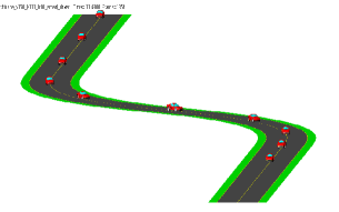
(a) The chicane maneuver.

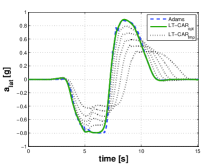
(b) Lateral acceleration $a_{lat}$.

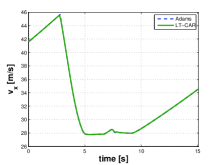
(c) Longitudinal velocity $v_{x}$.

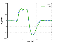
(d) Lateral velocity $v_{y}$.

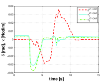
(e) Control inputs $\delta$(rad) and $\kappa$(Nodim).

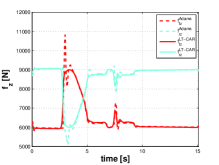
(f) Wheel load $f_{z}$.

Figure 6: Aggressive chicane maneuver. The dash and solid lines are the Adams and the optimal LT-CAR trajectories, respectively (except for the input plots that are given only for the LT-CAR). Temporary optimal trajectories are in light dot lines.

In Figure 6 we show the main plots of the first computation scenario. From the numerical computations we observed a fairly good position tracking. The position error was less than $0.1$ m. In Figure 6b we show the lateral acceleration profile followed by the LT-CAR model versus the Adams vehicle one. The light dot lines show the temporary optimal lateral accelerations obtained during the continuation updates. In Figure 6c and Figure 6d we report respectively the longitudinal and lateral speed profiles. The maximum error is less than $0.36$ m/s for the longitudinal speed and $0.07$ m/s for the lateral one. Comparing Figure 6f with Figure 6c, we may notice the relationship between the load transfer and the longitudinal acceleration (velocity slope). The vehicle enters the first turn decreasing the speed (constant negative slope) and the front load suddenly increases due to the load transfer induced by the strong braking. After the first turn the velocity is slightly increased (constant positive slope) as well as the load on the rear. Entering the second turn, the vehicle reduces its speed again and then accelerates out again.

It is worth noting in Figure 6f how the LT-CAR load transfer follows accurately the Adams vehicle load transfer except for a high frequency oscillation (probably due to the Adams suspensions transient). We stress the fact that there is an accurate prediction of the load transfer although the LT-CAR has not a suspension model.

IV-C Constant speed maneuver on a real testing track

In this test the desired maneuver consists of following a real testing track at constant speed. In particular, we choose a desired speed that in the last turn gives a lateral acceleration exceeding the tire limits. For this reason we compute the desired curve as the quasi-static trajectory of the Linear Tires LT-CAR model, (LT)²-CAR, on the desired path profile depicted in Figure 7a with velocity $v=30$ m/s.

The exploration strategy for this maneuver is as follows. To morph to the desired curve, we start with a speed of $25$ m/s and increase the velocity profile of $1$ m/s at each step. For each speed value, we compute the desired curve as the quasi-static trajectory of the (LT)²-CAR model on the track. As mentioned before, for the (LT)²-CAR model we can find the quasi-static trajectory on a wider range of lateral accelerations. The exploration strategy thus follows the usual steps. In the following pseudo code we denote $\xi_{\text{LT${}^{2}$-CAR}}^{v}$ the quasi-static trajectory of LT²-CAR obtained on the given path at constant velocity $v$.

Algorithm 4 Exploration strategy for the constant speed maneuver

0:  desired path $x_{d}(\cdot)$, $y_{d}(\cdot)$ and $v_{d}(\cdot)\equiv 30$m/s

  compute: desired curve $\xi_{d}=\xi_{\text{LT${}^{2}$-CAR}}^{30\text{m/s}}$;compute: initial trajectory $\xi_{0}^{25}=\mathcal{P}(\xi_{\text{LT${}^{2}$-CAR}}^{25\text{m/s}})$.

  for $v=25,\ldots,30$ m/s do

     set: $\xi_{d}^{v}=\xi_{\text{LT${}^{2}$-CAR}}^{v}$;

     compute: $\xi_{opt}^{v}$ = PO_Newt($\xi_{0}^{v}$, $\xi_{d}^{v}$);

     set: $\xi_{0}^{v+1}=\xi_{opt}^{v}$;

  end for

  $\xi_{opt}=\xi_{opt}^{30}$.

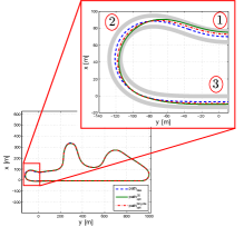
(a) Path $x$-$y$.

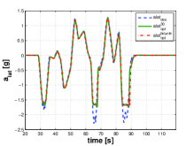
(b) Lateral acceleration $a_{lat}$.

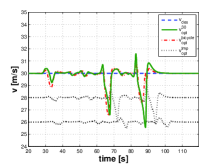
(c) Velocity $v$.

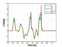
(d) Sideslip $\beta$.

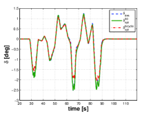
(e) Steer angle $\delta$.

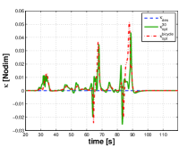
(f) Longitudinal slip $\kappa$.

Figure 7: Constant speed ($30m/s$) maneuver on a real testing track. The dash, solid and dash-dot lines are the desired curve, the optimal LT-CAR and the optimal bicycle model trajectories, respectively. Temporary optimal trajectories (for $v=26,28$ m/s) are in light dot lines.

In Figures 7 the optimal trajectory of the LT-CAR model (solid green) is compared with the desired curve (dash blue) and with the optimal trajectory of the bicycle model (dash-dot red). We choose a desired speed ($30$ m/s) that in the last turn gives a lateral acceleration exceeding the tire limits. The comparison with the bicycle model confirms the importance of including the load transfer. Indeed, the behavior of the two models is significantly different in the braking and acceleration regions, Figure 7f. In particular, in the last turn, the vehicle decelerates in order to satisfy the maximum acceleration limit. Notice that both the two models achieve this limit, Figure 7b. However, the LT-CAR has to anticipate the breaking point and increase the value of the longitudinal slip with respect to the bicycle model, Figure 7f. This behavior is due to the load transfer: in the LT-CAR the weight shifts to the front axle, thus reducing the traction capability. The behavior is reversed in the acceleration region. Notice that, in order to achieve the maximum lateral acceleration, the LT-CAR requires a lower sideslip angle, but a higher steer angle, Figures 7d and 7e. Next, we comment on an interesting phenomenon happening in the last turn. In the first straight portion (highlighted with “$1$” in Figure 7a), the vehicle moves to the right of the track to reduce the path curvature when entering the turn. In order to generate the required lateral forces in the turn (portion “$2$”) the tires have a high sideslip angle, Figure 7d. When the car starts to exit the turn (portion “$3$”), the lateral forces on the tires decrease, so that the longitudinal slip can increase, Figure 7f, to regain the desired constant speed.

V Conclusions

In this paper we studied the problem of modeling and exploring the dynamics of a single-track rigid car model that takes into account tire models and load transfer. Starting from the bicycle model, we introduced the load transfer phenomenon by explicitly imposing the holonomic constraints for the contact with the ground. The resulting model shows many of the interesting dynamic effects of a real car. For this rigid car model we characterized the equilibrium manifold on the entire range of operation of the tires and analyzed how it changes with respect to suitable parameters. Finally, we provided a strategy, based on nonlinear optimal control techniques and continuation methods, to explore the trajectories of the car model. Specifically, the proposed exploration strategy provides an effective approach for exploring the limits of the vehicle. The strategy was used, e.g., to find trajectories in which the lateral acceleration limit of the vehicle is reached, without applying constrained optimal control methods. We provided numerical computations showing the effectiveness of the exploration strategy on an aggressive maneuver and a real testing track.

-A Car model parameters

The tire equations introduced in Section II-A are based on the formulation in [27]. The pure longitudinal and lateral slips are given by

$$\begin{split}f_{x0}(\kappa)&=d_{x}\sin{\{c_{x}\arctan{[b_{x}\kappa-e_{x}(b_{x}\kappa-\arctan{b_{x}\kappa})]}\}},\\ f_{y0}(\beta)&=d_{y}\sin{\{c_{y}\arctan{[b_{y}\beta-e_{y}(b_{y}\beta-\arctan{b_{y}\beta})]}\}}\end{split}$$

and the loss functions for combined slips by

$$\begin{split}g_{x\beta}(\kappa,\beta)&=\cos{\biggl{[}c_{x\beta}\arctan{\Bigl{(}\beta\frac{r_{bx1}}{1+r^{2}_{bx2}\kappa^{2}}\Bigr{)}}\biggr{]}},\\ g_{yk}(\kappa,\beta)&=\cos{\biggl{[}c_{yk}\arctan{\Bigl{(}\kappa\frac{r_{by1}}{1+r^{2}_{by2}\beta^{2}}\Bigr{)}}\biggr{]}}.\end{split}$$

The parameters are based on the ones given in [25]. The tire parameters are determined by nonlinear curve-fitting routines.
Sports car $$\footnotesize{\begin{array}[]{llllll}{}&~{}~{}\mbox{rear}&~{}~{}\mbox{front}&{}&~{}~{}\mbox{rear}&~{}~{}\mbox{front}\\ d_{x}&\phantom{-}1.688&\phantom{-}1.688&d_{y}&\phantom{-}1.688&\phantom{-}1.688\\[3.44444pt] c_{x}&\phantom{-}1.65&\phantom{-}1.65&c_{y}&\phantom{-}1.79&\phantom{-}1.79\\ b_{x}&\phantom{-}8.22&\phantom{-}8.22&b_{y}&\phantom{-}8.822&\phantom{-}12.848\\ e_{x}&\phantom{-}-10.0&\phantom{-}-10.0&e_{y}&-2.02&-1.206\\[3.44444pt] c_{x\beta}&\phantom{-}1.1231&\phantom{-}1.1231&c_{y\kappa}&\phantom{-}1.0533&\phantom{-}1.0533\\ r_{bx1}&\phantom{-}13.476&\phantom{-}13.476&r_{by1}&\phantom{-}7.7856&\phantom{-}7.7856\\ r_{bx2}&\phantom{-}11.354&\phantom{-}11.354&r_{by2}&\phantom{-}8.1697&\phantom{-}8.1697\\ \end{array}}$$ $$a=1.421[m]\quad b=1.029[m]\quad h=0.42[m]$$ $$m=1480[kg]\quad I_{b}=\left[\begin{array}[]{ccc}590&0&-50\\ 0&1730&0\\ -50&0&1950\end{array}\right]$$ Adams model $$\footnotesize{\begin{array}[]{llllll}{}&~{}~{}\mbox{rear}&~{}~{}\mbox{front}&{}&~{}~{}\mbox{rear}&~{}~{}\mbox{front}\\ d_{x}&\phantom{-}1.48&\phantom{-}1.48&d_{y}&\phantom{-}1.22&\phantom{-}1.22\\[3.44444pt] c_{x}&\phantom{-}1.37&\phantom{-}1.37&c_{y}&\phantom{-}1.25&\phantom{-}1.25\\ b_{x}&\phantom{-}18.22&\phantom{-}18.22&b_{y}&\phantom{-}17.8&\phantom{-}17.8\\ e_{x}&-0.46&-0.46&e_{y}&\phantom{-}0.02&\phantom{-}0.02\\[3.44444pt] c_{x\beta}&\phantom{-}1.1231&\phantom{-}1.1231&c_{y\kappa}&\phantom{-}1.0533&\phantom{-}1.0533\\ r_{bx1}&\phantom{-}13.476&\phantom{-}13.476&r_{by1}&\phantom{-}7.7856&\phantom{-}7.7856\\ r_{bx2}&\phantom{-}11.354&\phantom{-}11.354&r_{by2}&\phantom{-}8.1697&\phantom{-}8.1697\\ \end{array}}$$ $$a=1.48[m]\quad b=1.08[m]\quad h=0.43[m]$$ $$m=1528.68[kg]\quad I_{b}=\left[\begin{array}[]{ccc}583.39&0&-1.91\\ 0&6129.12&0\\ -1.91&0&6022.36\end{array}\right]$$

-B Proof of Proposition II.3

This appendix gives the main steps for the derivation of the constrained Lagrangian dynamics.

To prove statement (i), we use Lagrange’s equations (1) including all the coordinates (even the constrained ones) and plug the constraints directly into the equations of motion (rather than attempting to eliminate the constraints by an appropriate choice of coordinates). The constraints are taken into account by adding the constraint forces into the equation of motion as additional forces which affect the motion of the system. Hence the constrained equations of motion can be written as

$$\begin{split}M(q)\ddot{q}+C(q,\dot{q})+G(q)&=J^{T}_{f}(q)f-A^{T}(q)\lambda\\ A(q)\ddot{q}+\dot{A}(q)\dot{q}&=0,\end{split}$$

where $M$, $C$, $G$ and $A$ are the one introduced in (2) and (3). The constraints lead to $q_{c}(t)=\dot{q}_{c}(t)=\ddot{q}_{c}(t)=0$, $\forall t\in{\mathbb{R}}$, so that we have

$$[M(q)\ddot{q}+C(q,\dot{q})+G(q)]|_{q_{c}=0}=[J^{T}_{f}(q)f-A^{T}(q)\lambda]|_{q_{c}=0}$$

where

$$M(q)|_{q_{c}=0}=\left[\begin{array}[]{c|c}M_{1}(q_{r})&M_{2}(q_{r})\end{array}\right]=\left[\begin{array}[]{ccc|cc}m&0&-mbs_{\psi}&0&-mhc_{\psi}\\ 0&m&mbc_{\psi}&0&-mhs_{\psi}\\ -mbs_{\psi}&mbc_{\psi}&mb^{2}+I_{zz}&0&0\\ 0&0&0&m&mb\\ -mhc_{\psi}&-mhs_{\psi}&0&mb&I_{yy}+m(b^{2}+h^{2})\\ \end{array}\right]$$

$$A(q)|_{q_{c}=0}=\left[\begin{array}[]{ccccc}0&0&0&1&-(a+b)\\ 0&0&0&1&0\\ \end{array}\right]\,,$$

and $C(q,\dot{q})|_{q_{c}=0}$, $G(q)|_{q_{c}=0}$, $J^{T}_{f}(q)f|_{q_{c}=0}$ are given by (5), and (6) respectively. We rewrite the equations of motion with respect to the extended variables $[q_{r},\lambda]^{T}$ as

$$[M_{1}(q_{r})|A^{T}]\left[\begin{array}[]{cc}\ddot{q}_{r}\\ \lambda\\ \end{array}\right]\,+\mathcal{C}(q_{r},\dot{q}_{r})+\mathcal{G}(q_{r})=\left[\begin{array}[]{c}\mathcal{U}_{1}\\ \hline\cr 0\end{array}\right].$$ (20)

Defining $\tilde{\mathcal{M}}=[M_{1}(q_{r})|A^{T}]$, the special structure (4) follows.

To prove statement (ii), we compute the reduced Lagrangian $\mathcal{L}_{r}(q_{r})=T(q_{r},\dot{q}_{r})-V(q_{r})$ and derive the Euler-Lagrange equations. Explicit calculations, shown in Appendix -C, lead to equation (7). The expression of the constraint forces follows from the arguments to prove statement (i).

Finally, to prove (iii), if the forces $f$ depend linearly on the reaction forces we have $f=F\lambda$, for a suitable $F$, then we can rewrite the generalized forces as

$$\biggl{[}\begin{array}[]{c}\mathcal{U}_{1}\\ \hline\cr 0\end{array}\biggr{]}=J^{T}_{f}(q_{r})|_{q_{c}=0}\left[\begin{array}[]{cc}\mu_{fx}&0\\ \mu_{fy}&0\\ 0&\mu_{rx}\\ 0&\mu_{ry}\\ \end{array}\right]\lambda=\begin{bmatrix}c_{\psi}\mu_{fx}-s_{\psi}\mu_{fy}&c_{\psi}\mu_{rx}-s_{\psi}\mu_{ry}\\ s_{\psi}\mu_{fx}+c_{\psi}\mu_{fy}&s_{\psi}\mu_{rx}+c_{\psi}\mu_{ry}\\ (a+b)\mu_{fy}&0\\ \hline\cr 0&0\\ 0&0\\ \end{bmatrix}\lambda:=\left[\begin{array}[]{c}\mathcal{M}_{12}\\ \hline\cr 0\\ \end{array}\right]\lambda,$$

so that equation (20) becomes

$$\tilde{\mathcal{M}}(q_{r})\left[\begin{array}[]{c}\ddot{q}_{r}\\ \lambda\\ \end{array}\right]-\left[\begin{array}[]{c|c}0&\mathcal{M}_{12}(q_{r},\mu)\\ \hline\cr 0&0\end{array}\right]\left[\begin{array}[]{c}\ddot{q}_{r}\\ \lambda\\ \end{array}\right]+\mathcal{C}+\mathcal{G}=0$$

from which equation (8) follows directly.

-C Reduced order model without load transfer (bicycle model)

The vector $q_{r}=[x,y,\psi]^{T}$ provides a valid set of generalized coordinates for dynamics calculations. So, the equations of motion for a Single-track rigid car with generalized coordinates $q_{r}=[x,y,\psi]^{T}$ are given by

$$\mathcal{M}_{11}(q_{r})\ddot{q_{r}}+\mathcal{C}_{1}(q_{r},\dot{q}_{r})+\mathcal{G}_{1}(q_{r})=\mathcal{U}_{1}$$

where the mass matrix, the Coriolis and gravity vectors are

$$\mathcal{M}_{11}(q_{r})=\left[\begin{array}[]{ccc}m&0&-mbs_{\psi}\\ 0&m&mbc_{\psi}\\ -mbs_{\psi}&mbc_{\psi}&(I_{zz}+mb^{2})\\ \end{array}\right],\,\mathcal{C}_{1}(q_{r},\dot{q}_{r})=\left[\begin{array}[]{c}-mbc_{\psi}\dot{\psi}^{2}\\ -mbs_{\psi}\dot{\psi}^{2}\\ 0\\ \end{array}\right],\,\mathcal{G}_{1}(q_{r})=\left[\begin{array}[]{c}0\\ 0\\ 0\\ \end{array}\right]$$

and the vector of generalized forces is

$$\mathcal{U}_{1}=J_{f}^{T}(\psi)f=\left[\begin{array}[]{cccccc}c_{\psi}&-s_{\psi}&c_{\psi}&-s_{\psi}\\ s_{\psi}&c_{\psi}&s_{\psi}&c_{\psi}\\ 0&(a+b)&0&0\\ \end{array}\right]\left[\begin{array}[]{c}f_{fx}\\ f_{fy}\\ f_{rx}\\ f_{ry}\end{array}\right].$$

-D Projection Operator Newton method

We recall the optimal control tools, namely the Projection Operator-based Newton method, used to explore the trajectory manifold of the car vehicle, see [26] and [32]. We are interested in solving optimal control problems of the form

$$\begin{split}\min&\;\;h(\xi;\xi_{d})\!:=\!\frac{1}{2}\!\!\int_{0}^{T}\!\!\!\!\|x(\tau)\!-\!x_{d}(\tau)\|_{Q}^{2}+\|u(\tau)\!-\!u_{d}(\tau)\|_{R}^{2}d\tau+\frac{1}{2}\|x(T)-x_{d}(T)\|_{P_{1}}^{2}\\ \!\text{subj. \!to}&\;\;\dot{x}=f(x,u)\qquad x(0)=x_{0},\end{split}$$

with $\xi=(x(\cdot),u(\cdot))$ and $\xi_{d}=(x_{d}(\cdot),u_{d}(\cdot))$. Denoting $\mathcal{T}$ the manifold of bounded trajectories $(x(\cdot),u(\cdot))$ on $[0,T]$, the optimization problem can be written as

$$\min_{\xi\in\mathcal{T}}h(\xi;\xi_{d}).$$ (21)

The Projection Operator Newton method is based on a trajectory tracking approach, defining a projection operator that maps a state-control curve (e.g., a desired curve) onto the trajectory manifold. Specifically, the time varying-trajectory tracking control law

$$\begin{split}\dot{x}(t)=&f(x(t),u(t)),\qquad x(0)=x_{0},\\ u(t)=&\mu(t)+K(t)(\alpha(t)-x(t))\end{split}$$ (22)

defines the projection operator

$$\mathcal{P}:\xi=(\alpha(\cdot),\mu(\cdot))\mapsto\eta=(x(\cdot),u(\cdot)),$$

mapping the curve $\xi$ to the trajectory $\eta$.

Using the projection operator to locally parametrize the trajectory manifold, we may convert the constrained optimization problem (21) into one of minimizing the unconstrained functional $g(\xi;\xi_{d})=h(P(\xi);\xi_{d})$ using, for example, a Newton descent method as described below. A geometric representation of the projection operator is shown in Figure 8.

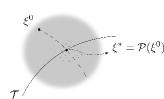
Figure 8: Geometric representation of the trajectory manifold: every point of $\mathcal{T}$ is a trajectory of the system. The projection of the curve $\xi^{0}=(\alpha(\cdot),\mu(\cdot))$ on $\mathcal{T}$ through $\mathcal{P}$ is the trajectory $\xi^{*}=(\textrm{x}(\cdot),\textrm{u}(\cdot))$.

Minimization of the trajectory functional is accomplished by iterating over the algorithm shown in the table, where $\xi_{i}$ indicates the current trajectory iterate, $\xi_{0}$ an initial trajectory, and $\zeta\mapsto Dg(\xi_{i};\xi_{d})\cdot\zeta$ and $\zeta\mapsto D^{2}g(\xi_{i};\xi_{d})(\zeta,\zeta)$ are respectively the first and second Fréchet differentials of the functional $g(\xi)=h(\mathcal{P}(\xi);\xi_{d})$ at $\xi_{i}$.

Projection operator Newton method (PO_Newt)
Given initial trajectory $\xi_{0}\in\mathcal{T}$
For $i=0,1,2...$

• design $K$ defining $\mathcal{P}$ about $\xi_{i}$

• search for descent direction

  $$\zeta_{i}=\text{arg}\min_{\zeta\in T_{\xi_{i}}\mathcal{T}}Dg(\xi_{i};\xi_{d})\cdot\zeta+\frac{1}{2}D^{2}g(\xi_{i};\xi_{d})(\zeta,\zeta)$$

• step size $\gamma_{i}=\arg\min_{\gamma\in(0,1]}g(\xi+\gamma\zeta_{i})$;

• project $\xi_{i+1}={\mathcal{P}}(\xi_{i}+\gamma_{i}\zeta_{i})$.

end

The algorithm has the structure of a standard Newton method for the minimization of an unconstrained function. The key points are the design of $K$ defining the projection operator and the computation of the derivatives of $g$ to “search for descent direction”. It is worth noting that these steps involve the solution of well known linear quadratic optimal control problems [26].

References

- [1] A. Rucco, G. Notarstefano, and J. Hauser, “Dynamics exploration of a single-track rigid car model with load transfer,” in IEEE Conf. on Decision and Control, Atlanta, GA, USA, December 2010, pp. 4934–4939.
- [2] T. D. Day, “An overview of the HVE vehicle model,” in SAE, paper no. 950308, 1995, pp. 55–68.
- [3] R. Frezza and A. Beghi, “A virtual motorcycle driver for closed-loop simulation,” IEEE Control Systems Magazine, vol. 5, pp. 62–77, 2006.
- [4] W. F. Milliken and D. L. Milliken, Race car vehicle dynamics. SAE International, 1995.
- [5] T. D. Gillespie, Fundamentals of Vehicle Dynamics. SAE, Warrendale, 1992.
- [6] J. Y. Wong, Theory of ground vehicles. John Wiley & Sons, 2001.
- [7] U. Kiencke and L. Nielsen, Automotive Control Systems for Engine, Driveline, and Vehicle. Springer Verlag, 2005.
- [8] R. Rajamani, Vehicle Dynamics and Control. Springer, 2006.
- [9] E. Velenis, P. Tsiotras, and J. Lu, “Optimality properties and driver input parameterization for trail-braking cornering,” European Journal of Control, vol. 14, no. 4, pp. 308–320, 2008.
- [10] E. Velenis, E. Frazzoli, and P. Tsiotras, “Steady-state cornering equilibria and stabilization for a vehicle during extreme operating conditions,” International Journal of Vehicle Autonomous Systems, vol. 8, no. 2–4, 2010.
- [11] E. Ono, S. Hosoe, H. D. Tuan, and S. Doi, “Bifurcation in vehicle dynamics and robust front wheel steering control,” IEEE Transactions on Control Systems Technology, vol. 6, no. 3, pp. 412–420, 1998.
- [12] M. Abdulrahim, “On the dynamics of automobile drifting,” in SAE Technical Paper 2006-01-1019, 2006.
- [13] E. Frazzoli, “Discussion on ‘Optimality properties and driver input parameterization for trail-braking cornering’,” European Journal of Control, vol. 14, no. 4, pp. 321–324, July-August 2008.
- [14] J. Yi, J. Li, J. Lu, and Z. Liu, “On the stability and agility of aggressive vehicle maneuvers: A pendulum-turn maneuver example,” IEEE Transactions on Control Systems Technology, vol. PP, no. 99, pp. 1 –14, 2011.
- [15] D. Casanova, R. Sharp, and P. Symonds, “Minimum time manoeuvring: The significance of yaw inertia,” Vehicle System Dynamics, vol. 34, no. 2, pp. 77–115, 2000.
- [16] F. Kehrle, F. J.V., C. Kirches, and S. Sager, “Optimal control of formula 1 race cars in a vdrift based virtual environment,” in IFAC World Congress Milan, 2011.
- [17] D. Casanova, R. Sharp, and P. Symonds, “On minimum time optimisation of formula one cars: the influence of vehicle mass,” in In Proceedings of International Symposium on Advanced Vehicle Control, Ann Arbor, Michigan, 2000.
- [18] ——, “On the optimisation of the longitudinal location of the mass centre of a formula one car for two circuits,” in In Proceedings of International Symposium on Advanced Vehicle Control, Hiroshima, Japan, 2002.
- [19] S. Anderson, S. Peters, T. Pilutti, and K. Iagnemma, “An optimal-control-based framework for trajectory planning, threat assessment, and semi-autonomous control of passenger vehicles in hazard avoidance scenarios,” International Journal of Vehicle Autonomous Systems, vol. 8, pp. 190–216, 2010.
- [20] P. Falcone, F. Borrelli, J. Asgari, H. E. Tseng, and D. Hrovat, “Predictive active steering control for autonomous vehicle systems,” IEEE Transactions on Control Systems Technology, vol. 15, no. 3, pp. 566–580, 2007.
- [21] P. Falcone, M. Tufo, F. Borrelli, J. Asgari, and H. Tseng, “A linear time varying model predictive control approach to the integrated vehicle dynamics control problem in autonomous systems,” in IEEE Conf. on Decision and Control, New Orleans, LA, 2007, pp. 2980 – 2985.
- [22] P. MacMillin and J. Hauser, “Development and exploration of a rigid motorcycle model,” in IEEE Conf. on Decision and Control, Shanghai, China, Dec. 2009, pp. 4396–4401.
- [23] A. Saccon, J. Hauser, and A. Beghi, “Trajectory exploration of a rigid motorcycle model,” IEEE Transactions on Control Systems Technology, vol. 20, no. 2, pp. 424 –437, march 2012.
- [24] E. L. Allgower and K. Georg, Numerical continuation methods: an introduction. Springer-Verlag New York, Inc., 1990.
- [25] G. Genta, Motor vehicle dynamics: modeling and simulation. World Scientific, 2006.
- [26] J. Hauser, “A projection operator approach to the optimization of trajectory functionals,” in IFAC World Congress, Barcelona, 2002.
- [27] H. B. Pacejka, Tire and Vehicle dynamics. Butterworth Heinemann, 2002.
- [28] R. Frezza, A. Beghi, and G. Notarstefano, “Almost kinematic reducibility of a car model with small lateral slip angle for control design,” in IEEE International Symposium on Industrial Electronics, Dubrovnik, June 2005, pp. 343–348.
- [29] C. Canudas de Wit, H. Olsson, K. J. Astrom, and P. Lischinsky, “A new model for control of systems with friction,” IEEE Transactions on Automatic Control, vol. 40(3), pp. 419–425, 1995.
- [30] C. Canudas de Wit, P. Tsiotras, E. Velenis, M. Basset, and G. Gissinger, “Dynamic friction models for road/tire longitudinal interaction,” Vehicle System Dynamics, vol. 39, no. 3, pp. 189–226, 2003.
- [31] M. W. Hirsch, Differential topology. Springer, New York, 1997.
- [32] J. Hauser and D. G. Meyer, “The trajectory manifold of a nonlinear control system,” in IEEE Conf. on Decision and Control, vol. 1, December 1998, pp. 1034–1039.