Random pinning in glassy spin models with plaquette interactions

Abstract

We use a random pinning procedure to study amorphous order in two glassy spin models. On increasing the concentration of pinned spins at constant temperature, we find a sharp crossover (but no thermodynamic phase transition) from bulk relaxation to localisation in a single state. At low temperatures, both models exhibit scaling behaviour. We discuss the growing length and time scales associated with amorphous order, and the fraction of pinned spins required to localize the system in a single state. These results, obtained for finite dimensional interacting models, provide a theoretical scenario for the effect of random pinning that differs qualitatively from previous approaches based either on mean-field, mode-coupling, or renormalization group treatments.

I Introduction

Supercooled liquids and glasses have very large relaxation times and complex relaxation mechanisms, but their structures appear disordered and unremarkable Ediger et al. (1996); Debenedetti and Stillinger (2001); Berthier and Biroli (2011). This combination is surprising and rather mysterious, especially because several recent studies Bouchaud and Biroli (2004); Montanari and Semerjian (2006); Kurchan and Levine (2011) indicate that if a relaxation time increases sufficiently rapidly on cooling then this must be accompanied by the development of some kind of structural order. The idea of growing amorphous order is that the diversity of amorphous states, as quantified by the configurational part of the entropy, decreases at low temperatures. This leads to increasing static correlation lengthscales, which can be measured using point-to-set correlations Bouchaud and Biroli (2004); Montanari and Semerjian (2006); Cavagna et al. (2007); Biroli et al. (2008); Kurchan and Levine (2011); Kob. et al. (2011); boo . If these length scales are large, the system may be localized into a single amorphous state by fixing the positions of a small fraction of the particles ber ; cam . This localization occurs at temperatures above the glass transition temperature, so the pinning procedure bypasses the challenging task of thermalizing systems at very low temperatures.

Here, we investigate amorphous order in two finite dimensional interacting spin systems. These are the square plaquette model (SPM) Lipowski (1997) and the triangular plaquette model (TPM) Newman and Moore (1999). They both have growing relaxation times at low temperatures, but two-point thermodynamic correlation functions do not indicate the presence of any growing length scale Garrahan (2002), and the models do not have phase transitions at any finite temperature. Additionally, structural relaxation at low temperatures exhibits strong dynamical heterogeneity and growing dynamic lengthscales Jack et al. (2005); Jack and Garrahan (2005). These features mimic those of supercooled liquids, but the models are numerically and analytically more tractable than off-lattice particle systems. This makes them useful models for studying generic features of glassy systems Buhot and Garrahan (2002); Jack et al. (2005); Jack and Garrahan (2005); pla .

Several methods have been proposed for characterizing amorphous order. A prominent recent example is to fix particles everywhere except within a small cavity, and then to study the motion of particles within this cavity Bouchaud and Biroli (2004); Cavagna et al. (2007); Biroli et al. (2008); Sausset and Levine (2011); ber . Other possible measurements of amorphous order involve freezing spins in a different geometrical arrangement Kob. et al. (2011); ber , or direct measurement of the diversity of amorphous packings Kurchan and Levine (2011); Sausset and Levine (2011). Here we follow Kim (2003); cam ; ber ; pro ; tar and fix a fraction $f$ of particles (or spins), distributed randomly through the system in the positions (or orientations) that are representative of thermal equilibrium. In supercooled liquids, a thermodynamic phase transition on varying $f$ was recently predicted cam , based on an analysis within random first-order transition (RFOT) theory Kirkpatrick and Thirumalai (1987); Kirkpatrick et al. (1989). Another recent analysis based on mode-coupling theory predicts a dynamic singularity on varying $f$ Krakoviack (2011). Numerical studies Kim (2003); ber ; pro ; tar have mainly addressed the behaviour at low to moderate pinning fraction $f$, leaving open the question of the existence of phase transitions at larger $f$.

Here, we explore the effect of random pinning in the plaquette models, concentrating on the behaviour at the relatively large pinning fractions where phase transitions are predicted to occur in supercooled liquids. We show that the plaquette models do not exhibit thermodynamic phase transitions on varying $f$ at any finite temperature. However, we do find a well-defined crossover from ‘bulk’ behaviour (where the system explores a large number of configurations), to ‘frozen’ behaviour (where the system remains trapped in a region of configuration space) occurring at some finite fraction $f^{*}$. As the temperature is reduced, the crossover occurs at an increasingly small value of $f^{*}$, and becomes increasingly sharp.

From previous studies of point-to-set correlations in closed cavities for plaquette models Jack and Garrahan (2005), it is known that these models do have growing amorphous order at low temperatures, but their behaviour is not consistent with RFOT. The results we present here therefore illustrate a theoretical scenario, alternative to mode-coupling and RFOT treatments, for understanding the behaviour of model supercooled liquids with randomly pinned particles.

After defining our models in Sec. II, we show numerical results for this crossover in Sec. III. In Sec. IV we investigate the length scales that characterize amorphous order in the system, including their scaling with temperature. In Sec. V we use analytic arguments in the SPM to study the small-$f$ behaviour, and the behaviour near the crossover. Finally in Sec. VI we discuss the interpretation of our results, including their relation to previous theoretical analysis.

II Plaquette models

II.1 Definitions

The plaquette models consist of Ising spins, $s_{i}=\pm 1$, on a lattice, interacting through either three- or four-body terms. They evolve dynamically through single spin-flips with Metropolis rates, $w_{i}=\min(1,\mathrm{e}^{-\beta\Delta E_{i}})$, where $\Delta E_{i}$ is the change in energy of the system on flipping spin $i$ and $\beta\equiv 1/T$ is the inverse temperature.

The energy of the square plaquette model (SPM) is

$$E=-\frac{1}{2}\sum_{\square}s_{1}s_{2}s_{3}s_{4},$$ (1)

where the sum runs over plaquettes of the square lattice Lipowski (1997); Garrahan (2002). It is useful to define $c\equiv\mathrm{e}^{-\beta}$, since length and time scales typically show power law scaling with $c$ in the low temperature limit ($c\to 0$). The model has a dual representation in terms of ‘defect’ variables, $n_{p}=(1-s_{1}s_{2}s_{3}s_{4})/2$, which are associated with the plaquettes $p$ of the square lattice. In terms of these defect variables, the thermodynamic properties of the system are those of a non-interacting lattice gas with $\langle n_{p}\rangle=(1+\mathrm{e}^{\beta})^{-1}$ approximately equal to $c$ at low temperatures. We use square systems with periodic boundaries.

The energy of the triangular plaquette model (TPM) is

$$E=-\frac{1}{2}\sum_{\nabla}s_{1}s_{2}s_{3},$$ (2)

where the sum runs over downward pointing plaquettes of the hexagonal lattice Newman and Moore (1999). In this model, the defect variables are associated with these plaquettes, $n_{p}=(1-s_{1}s_{2}s_{3})/2$. We use rhombus-shaped systems with periodic boundaries. We always take the linear system size to be a power of 2, which minimizes finite size effects.

In the defect representation, both the SPM and the TPM have strong similarities with kinetically constrained models Ritort and Sollich (2003). In both systems, the thermodynamic free energy per spin (in the limit of large systems) is simply $-T\log[2\cosh(1/2T)]$. This is a smooth and unremarkable function of temperature down to $T=0$. However, the dynamical properties of the models, to be described shortly, are not trivial. This combination of simple thermodynamic properties and complex dynamics is consistent with the dynamic facilitation picture of the glass transition Chandler and Garrahan (2010).

II.2 Square plaquette model at $f=0$

Before considering the effect of pinning a fraction of spins, we first review some relevant results for the SPM with $f=0$, see Refs. Garrahan (2002); Jack et al. (2005) for more details. Symmetry under global spin reversal implies that $\langle s_{i}\rangle=0$, and all non-trivial two-point and three-point correlation functions also vanish. The simplest non-trivial correlation functions involve four spins. For spins $a,b,c,d$ lying on the four vertices of an $x\times y$ rectangle then

$$g_{\mathrm{s}}(x,y)\equiv\langle s_{a}s_{b}s_{c}s_{d}\rangle_{0}=\tanh(\beta/2)^{xy}.$$ (3)

All other non-trivial four-point correlations vanish.

The function $g_{\mathrm{s}}(x,y)$ has scaling behaviour at low temperatures. Full details are given in Sec. IV.2 below, but the essential points are that correlations are anisotropic and the model supports two correlation lengths at low temperatures. The shorter length is $\xi_{0}\sim c^{-1/2}$, and there is also a longer length $\xi\sim c^{-1}$ associated with the correlations along the lattice axis. We note that previous analysis of static correlations considered only the shorter of these two correlation lengths Jack et al. (2005).

Point-to-set correlations were considered in Ref. Jack and Garrahan (2005), for the case of an isotropic (square) cavity of linear size $r$. For $r\lesssim\xi_{0}\sim c^{-1/2}$, the configurational entropy of the cavity is close to zero. For $\xi_{0}\lesssim r\lesssim\xi\sim c^{-1}$, the cavity has strong finite size effects but its configurational entropy is non-zero and the spin-spin autocorrelation function decays to zero at the centre of the cavity. This implies that these larger cavities are no longer frozen in a single amorphous state, so we identify $\xi_{0}$ as the point-to-set length Jack and Garrahan (2005).

Dynamical observables in the square plaquette model also show scaling behaviour. The relaxation time for spins is $\tau\approx c^{-3}\sim\mathrm{e}^{3/T}$, consistent with the behaviour of ‘strong’ glass-formers Buhot and Garrahan (2002). Energy-energy correlations decay have relaxation times longer than $\tau$ at low temperatures, although they also have Arrhenius scaling. Four-point dynamic correlation functions, also discussed in more detail below, are anisotropic as well, with correlations being strongly localized along the axis of the square lattice, and having spatial on-axis extension of range $\xi\sim\mathrm{e}^{\beta}=c^{-1}$ Jack et al. (2005).

II.3 Triangular plaquette model at $f=0$

Static correlations in the TPM were discussed in Ref. Newman and Moore (1999) where it was shown that $\langle s_{i}\rangle=0$ and $\langle s_{i}s_{j}\rangle=\delta_{ij}$, as in the SPM. The relaxation time in the TPM has ‘fragile’ super-arrhenius scaling $\tau\sim\mathrm{e}^{1/(T^{2}\log 3)}$ Jack and Garrahan (2005), which arises from a hierarchy of mechanisms whose characteristic timescales increase as the logarithm of their associated lengthscales (see also Garrahan and Chandler (2003); Berthier and Garrahan (2005); Keys et al. (2011)). Static correlation lengths, point-to-set correlations, and dynamical four-point correlations are considered in Ref. Jack and Garrahan (2005), where it was found that the scaling of these functions all depend on a unique correlation lengthscale, $\xi\sim c^{-1/d_{\mathrm{f}}}$, where $d_{\mathrm{f}}=\log 3/\log 2\approx 1.585$ is the fractal dimension of the Sierpinski triangle. It was also found recently Sasa (2010) that the TPM supports unusual phase transitions if it is constrained to have a fixed non-zero magnetisation, but we do not discuss that case here.

III Effect of random pinning

We now turn to our main results, which correspond to the following thought-experiment cam ; Kim (2003); Kim et al. (2011); pro ; ber ; Krakoviack (2011). We select a reference configuration from a thermally equilibrated system and we instantaneously ‘freeze’ (or ‘pin’) at time $t=0$ the state of a finite set of spins. Each spin is frozen with probability $f$, independently of all other spins. The spins that are not frozen evolve with Monte-Carlo (MC) dynamics for some time $t$, after which various measurements are performed.

III.1 Correlation functions and susceptibilities

To describe these measurements, we first establish our notations and define the correlation functions and susceptibilities that we will consider. The system consists of $V$ spins $s_{i}=\pm 1$, with $i=1,\dots,V$. To describe whether a spin is frozen, we introduce the binary variables $f_{i}$, with $f_{i}=1$ if spin $i$ is frozen, zero otherwise. We use angle brackets $\langle\cdots\rangle$ to denote averages which run over the reference configuration, the choice of frozen spins, and the MC dynamics. We also use $\langle\cdots\rangle_{0}$ to denote a ‘bulk’ thermal average, i.e. in the absence of any pinned particles ($f=0$).

It is convenient to define the autocorrelation of the mobile spins. For spin $i$, this is defined as $a_{i}(t)=(1-f_{i})s_{i}(t)s_{i}(0)$, and it takes values $0,\pm 1$. The number of mobile (unfrozen) spins is $\hat{N}_{\mathrm{m}}=\sum_{i}(1-f_{i})$, which is a fluctuating quantity within our analysis. We also define the (extensive) overlap $\hat{Q}(t)=\sum_{i}a_{i}(t)$ and the (intensive) autocorrelation function

$$C(t)=\frac{\langle\hat{Q}(t)\rangle}{\langle\hat{N}_{\mathrm{m}}\rangle}=\frac{\langle a_{i}(t)\rangle}{1-f}.$$ (4)

The four-point susceptibility quantifies the strength of spontaneous fluctuations of the overlap,

$$\chi_{4}(t)=\frac{\langle\delta\hat{Q}(t)^{2}\rangle}{\langle\hat{N}_{\mathrm{m}}\rangle}=\frac{\sum_{j}g_{4,ij}}{1-f},$$ (5)

and it is related to the volume integral of the four-point correlation function defined as

$$g_{4,ij}=\langle\delta a_{i}(t)\delta a_{j}(t)\rangle.$$ (6)

We use the notation $\delta O=O-\langle O\rangle$ for thermal fluctuations throughout this article.

In addition to the usual four-point correlations, we introduce three-point correlations and susceptibilities. We measure how the positions of the pinned spins are correlated with the states of mobile spins through the correlation

$$X_{ij}(t)=\langle\delta a_{i}(t)\delta f_{j}\rangle.$$ (7)

The ratio $(X_{ij}/f)$ measures the change in the average of $a_{i}$ if spin $j$ is assumed to be frozen. Hence,

$$\frac{\partial C(t)}{\partial f}=\frac{1}{f(1-f)^{2}}\sum_{j\neq i}X_{ij}.$$ (8)

To prove this relation, one writes $f=(1+\mathrm{e}^{\mu})^{-1}$, so that $\langle a_{i}(t)\sum_{j}\delta f_{j}\rangle=-\frac{\partial}{\partial\mu}\langle a_{i}(t)\rangle$, and Eq. (8) follows.

It is interesting to note that $X_{ij}(t)$ is an example of a three-point correlation function, and that $\frac{\partial C(t)}{\partial f}$ is therefore a three-point susceptibility, in the spirit of the dynamic functions introduced in Refs. Berthier et al. (2007a, b). Following Refs. Berthier et al. (2005); Berthier et al. (2007a, b) we can obtain a lower bound $\Delta\chi_{4}$ on the four-point susceptibility, $\chi_{4}(t)\geq\Delta\chi_{4}(t)$, which involves the three-point susceptibility defined above as

$$\Delta\chi_{4}(t)=f\left[(1-f)\frac{\partial C(t)}{\partial f}-C(t)\right]^{2}.$$ (9)

This relation is proved in Appendix A where we also show that a sufficient condition for saturation of the bound [i.e., $\chi_{4}(t)=\Delta\chi_{4}(t)$] is that for a given choice of frozen spins, the autocorrelations of the mobile spins are independent of each other and depend separately on the individual $f_{j}$. When this condition is obeyed, then the four-point correlation function may be expressed as a convolution of $X_{ij}$ with itself:

$$g_{4,ij}(t)\approx\frac{1}{f(1-f)}\sum_{k}X_{ik}(t)X_{jk}(t).$$ (10)

We refer to Appendix A for more details on this particular point.

Of particular interest is the limit of large time, $t\to\infty$, in which correlation functions become independent of the dynamical evolution of the system and may be calculated by equilibrium statistical mechanics. In this limit, we drop the time argument on our correlation functions, writing, as $t\to\infty$: $C(t)\to q$, $g_{4,ij}(t)\to g_{4,ij}$, $X_{ij}(t)\to X_{ij}$, and $\chi_{4}(t)\to\chi_{4}$. These limiting quantities are given by ‘static’ correlation functions. A general recipe for calculating them is given in Appendix A, which follows a similar analysis for off-lattice particle systems Krakoviack (2010). For small $f$, in particular, they may be calculated in a series expansion, see also Sec. V.

III.2 Numerical results

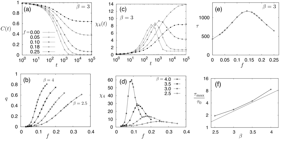
Figure 1: Overview of behaviour of the SPM with pinned spins. (a) Time-dependent correlation function $C(t)$ at inverse temperature $\beta=3$. (b) The long-time overlap $q=\lim_{t\to\infty}C(t)$ as a function of pinning fraction $f$ for four temperatures (the symbols are the same as those in panel e). (c) Time-dependent four-point susceptibility $\chi_{4}(t)$ at $\beta=3$. (d) Long-limit limit of $\chi_{4}$, for various temperatures. (e) Behaviour of the relaxation time on varying $f$ at $\beta=3$. (f) Behaviour of the maximal relaxation time $\tau_{\mathrm{max}}=\max_{f}\tau(f)$, normalised by the bulk relaxation time $\tau_{0}=\tau(f=0)$, as a function of inverse temperature. In practice $\tau_{\mathrm{max}}\approx\tau(f^{*})$. The straight line is $\tau_{\mathrm{max}}/\tau_{0}\propto\mathrm{e}^{\beta}$ which would imply $\tau_{\mathrm{max}}\propto\mathrm{e}^{4\beta}$. It is clear from the upwards curvature of the numerical data that $\tau_{\mathrm{max}}$ has a super-Arrhenius temperature dependence.

An overview of the influence of pinned spins on the SPM is shown in Fig. 1. In Fig. 1a we show that as $f$ is increased from zero, the long-time limit of $C(t)$ increases monotonically, since the frozen spins tend to maintain the system close to its initial state, preventing full relaxation of the autocorrelation function of the mobile spins. Thus, we confirm that by randomly freezing spins, the system crosses over from ‘bulk’ ergodic relaxation for $f=0$ to a nearly ‘frozen’ state at large $f$. Our goal is now to characterize this crossover further.

In Fig. 1b, we show the evolution of $q=q(f,T)$ with the fraction of pinned spins and temperature. As expected from Fig. 1a, the static value of the overlap increases monotonically with $f$ at any given temperature. More interesting is the temperature dependence of the $q(f,T)$ curves. We find that $q$ increases rapidly with decreasing temperature at constant $f$. This implies that for lower temperatures, a smaller amount of random pinning is required to localize the system in a single state. The interpretation is that the system has a greater degree of amorphous order at low temperatures.

Looking more closely at the $f$-dependence of $q$, the data in Fig. 1b indicate that $q(f,T)$ has an inflexion point at a characteristic value of the pinning fraction, $f=f^{*}$, so that the susceptibility $(\partial q/\partial f)$ is small both for small $f$ and for large $f$, with a well-defined maximum at $f^{*}(T)$. Thus we find that the bulk-to-localized crossover obtained with random pinning can be located by measuring the derivative of the static overlap. However, anticipating the discussion in Sec. VI, we note that $q(f,T)$ is a smooth function of $f$ with no sign of the sharp discontinuity that would be observed at a first order phase transition cam .

We next turn to fluctuations of the overlap, which we quantify via the four-point susceptibility $\chi_{4}(t)$. In Fig. 1c, we show the time evolution of $\chi_{4}(t)$ for different values of $f$, at constant temperature. For $f=0$, the susceptibility $\chi_{4}(t)$ has a peak for $t\approx\tau$, as usual in glassy systems boo . However, two features emerge when $f$ is increased. First, the time dependence changes dramatically: the maximum in $\chi_{4}(t)$ shifts to longer times until, for large $f$, the susceptibility $\chi_{4}(t)$ is monotonically increasing and saturates to a plateau at long times. This long time limit corresponds to the static susceptibility $\chi_{4}=\chi_{4}(f,T)$, proportional to the variance in the overlap $q(f,T)$. This increasing static susceptibility indicates that deviations between the final configuration and the initial (reference) configuration appear by cooperative processes involving many spins. Just like $(\partial q/\partial f)$, the static susceptibility $\chi_{4}$ goes through a maximum at the characteristic pinning fraction $f^{*}$.

Physically, the interpretation of the behaviour of $\chi_{4}(t)$ is as follows. When $f\ll f^{*}$, the system is in the bulk regime and easily escapes from the reference state through a process that is not very different from bulk relaxation. In this case, $\chi_{4}(t)$ is large near $t\approx\tau$, but it is small at long times since initial and final states are very different. When $f\gg f^{*}$, by contrast, there are so many frozen spins that the system is very constrained and few spins can relax. While the overlap is large, its fluctuations are necessarily quite small. For $f\approx f^{*}$, the number of frozen spins is just large enough to maintain the system near its initial state, and the overlap exhibits stronger fluctuations because the system ‘hesitates’ between both possibilities (“should I stay or should I go”). We discuss the spatial structure of these correlations in Sec. IV below.

We show in Fig. 1d the evolution of the static susceptibility $\chi_{4}$ with $f$ for different temperatures. As anticipated, the susceptibility goes through a maximum whose location and amplitude are strong functions of the temperature. On going to lower temperature, the peak of $\chi_{4}$ remains located near $f=f^{*}$ so it shifts towards smaller values of $f$; the amplitude of the peak increases rapidly, and its width decreases. Thus, the crossover between bulk and localized behaviours becomes sharper and more pronounced at low temperatures. A relevant conclusion for supercooled liquids is that the data in Fig. 1d show an increasing static susceptibility that measures the growth of amorphous order, but these data are obtained without any a priori knowledge of the many-body correlations that are responsible for this order. Thus, the random pinning procedure is a generic way to measure a growing static susceptibility in liquids approaching the glass transition, and offers a thermodynamic alternative to the measurement of relevant length scales via dynamic heterogeneity.

Turning to the dynamic behaviour in the presence of random pinning, we define a relaxation time $\tau=\tau(f,T)$ from the time decay of $C(t)$, via $\frac{C(\tau)-q}{1-q}=1/\mathrm{e}$. We compute $\tau$ using the data shown in Fig. 1a and show the results in Fig. 1e. We also find that $\tau$ has a non-monotonic behaviour, the relaxation being slowest near $f^{*}$. While the maximum is not very pronounced in Fig. 1e, we show in Fig. 1f that the ratio $\tau(f^{*},T)/\tau(f=0,T)$ increases when temperature is reduced. This is consistent with the presence of increasingly cooperative relaxation mechanisms in the presence of pinned spins. While the SPM without pinning has ‘strong’ glass scaling, $\tau(f=0)\sim\mathrm{e}^{3/T}$, we find that $\tau(f^{*})$ increases in a super-Arrhenius (fragile) fashion. This indicates that the relaxation mechanism for the system near $f^{*}$ is different from the bulk mechanism at $f=0$, presumably because the frozen spins act to frustrate relaxation of the mobile ones.

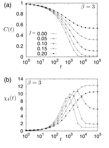
Figure 2: Effects of pinning in the TPM at $\beta=3$. (a) Time-dependent correlation function. (b) Time-dependent four-point susceptibility.

We expect many of the results shown for the SPM to be quite generic in glassy systems. Certainly, the behaviour in the TPM is similar. Figure 2 shows data for $C(t)$ and $\chi_{4}(t)$ in the TPM at the representative temperature $\beta=3$. As before, $C(t)$ exhibits a plateau at long times which increases with $f$, while the static susceptibility $\chi_{4}$ is maximal at some $f=f^{*}$. Consistent with the SPM, we also find that $f^{*}$ decreases at low temperature, that the maximum of the static susceptibilities increase, and that the time scales at $f^{*}$ increase. These results resemble strongly the ones shown in Fig. 1, and are therefore not shown, for brevity. However, the $f$-dependence of the relaxation time $\tau$ is weaker in the TPM than in the SPM: the ratio $\tau_{\mathrm{max}}/\tau_{0}$ does increase systematically on decreasing temperature but it takes values in the range $1-4$ while $\tau_{0}$ varies over nearly four orders of magnitude.

We emphasize that all of the results presented in this article are obtained in large systems and we have checked that they are free from finite size effects. In particular, susceptibilities and relaxation times have maxima at $f^{*}$ but the maximum values remain finite even when the thermodynamic limit is taken, $V\to\infty$. Thus, there are no diverging correlation times or correlation lengths in this system for any finite $f$ or $T$, nor is there any phase transition. However, we find that correlation times and susceptibilies have sharp maxima along a line $f^{*}(T)$ in the $(f,T)$ phase diagram.

IV Scaling of lengths

We have shown that varying $f$ in the SPM and TPM reveals crossovers at $f^{*}$, associated with maxima in susceptibilities and in relaxation times. We now discuss how these features can be related to correlation lengths in these systems. In particular, we focus on the scaling of these lengthscales at low temperatures.

IV.1 Visualisation of spatial correlations

It is instructive to visualise the spatial fluctuations that appear as a result of the random pinning. To this end, we consider the dynamic propensity Widmer-Cooper et al. (2004); Widmer-Cooper and Harrowell (2007). (Compared to visualising the autocorrelations $a_{i}$ directly, the propensity provides continuous functions rather than binary ones, and this yields images that better differentiate between regions where relaxation is frustrated by the frozen spins and those where relaxation can occur.)

To calculate the propensity, we take a single representative reference configuration, $\bm{s}^{\mathrm{A}}$, in which a specific set of spins are frozen, and we run several long MC trajectories starting from it. We calculate the autocorrelation $a_{i}(t)=s_{i}(t)s_{i}(0)$ for each unfrozen spin in each trajectory and we average over the trajectories to obtain the (site-dependent) propensities $p_{i}(t)=\overline{a_{i}(t)}$. For large times these propensities approach limiting values, $p_{i}=p_{i}(t\to\infty)$, which depend on the reference configuration $\bm{s}^{\mathrm{A}}$ but not on the time $t$. The propensities are therefore static on-site quantities characterizing the degree of freezing of spin $i$ for a given realization of the random pinning and a given reference configuration.

Figure 3: Snapshots of the propensities $p_{i}$ in the long-time limit. (a-c) SPM at $\beta=3$, varying $f$. At this temperature $f^{*}\approx 0.18$. (d-f) TPM at $\beta=3$ for which $f^{*}\approx 0.15$. Pinned spins are black while unpinned spins are color-coded with dark blue for $p_{i}\approx 1$, pale blue for $p_{i}\approx 0$ and green for $p_{i}\approx-1$. On increasing $f$, the spins become polarised so that $p_{i}\approx 1$ in most cases. The correlations associated with the propensity are strongest near $f^{*}$, consistent with $\chi_{4}$ being maximal.

Representative results are shown in Fig. 3, where pinned spins are shown in black, and a blue-green colour coding describes the propensity. Sites for which the pinned spins cause the configuration to remain near its initial state have $p_{i}\approx 1$ (dark blue) while those where the pinned spins have little effect have $p_{i}=0$ (light blue). If the frozen spins cause $s_{i}$ to become polarised in the opposite direction to $s_{i}^{\mathrm{A}}$, one finds $p_{i}<0$ (green).

At $f=0$ then $p_{i}=0$ for all $i$ and the system is homogeneous. As $f$ starts to increase (left panel), then the system acquires regions where the spins become polarised and cannot relax any more (coloured dark blue in Fig. 3). This seems to occur in small, isolated regions whose size increases with $f$. For $f\approx f^{*}$ (middle panel), these polarized regions percolate throughout the system and spatial fluctuations of the propensity occur over a large lengthscale. This yields snapshots where large regions are strongly polarised while others are unaffected by the pinning. Finally, as $f$ increases further above $f^{*}$ (right panel), most spins are strongly pinned, and only few small regions exist where motion remains possible. In this regime, the system is strongly localized near the reference configuration.

An important observation is that the lengthscales associated with these correlations observed near $f^{*}$ are much longer than the typical distance $f^{-1/2}$ between pinned spins. This is apparent in Fig. 3, because the coloured domains are clearly much larger than the spacing between (black) pinned sites. In other words, each correlated region in these images contain very many pinned spins. These observations will be quantified below in Sec. IV.3.

The qualitative description of these images is strongly reminiscent of observations made in dynamic heterogeneity studies boo , except that time has now been replaced by the fraction of pinned spins. The images in Fig. 3 suggest that a similar behaviour is found in both square and triangular models but that the specific features of the models will be reflected in the form of the correlation functions. For example, the SPM is characterized by strongly anisotropic correlations, while correlations appear more isotropic for the TPM, although they do have an underlying fractal structure. These observations once again echo previous studies of the dynamic heterogeneity in these models Jack et al. (2005)

IV.2 SPM: ‘Bulk’ scaling at $f=0$

To analyse length scales and their scaling in the SPM, it is useful to start by considering static correlations for the ‘bulk’ at $f=0$. As discussed in Sec. II, the first non-trivial correlations involve four spins arranged at the edges of a rectangle of size $x\times y$. It is clear from Eq. (3) that lines $xy=\mathrm{const.}$ are contours of the static four-point function $g_{\mathrm{s}}(x,y)$. That is, the four-spin correlations are strongly anisotropic, which leads to unusual scaling behaviour at low temperature ($c\to 0$). For example, one may measure correlations at a fixed finite angle $\theta$ to the lattice axes (with $\theta\neq 0,\pi/2$, etc), in which case

$$g_{\mathrm{s}}(x,y)\simeq G_{\mathrm{so}}(r\sqrt{c},\theta),$$ (11)

with $x=r\cos\theta$ and $y=r\sin\theta$, as usual. (Explicitly $G_{\mathrm{so}}(u,\theta)=\mathrm{e}^{-u^{2}\sin 2\theta}$.) Since the scaling variable is $u=r\sqrt{c}$, the correlation length away from the lattice axes scales as $1/\sqrt{c}$. (Throughout this section we use the symbol $G$ for scaling functions, with the approximate equalities valid on taking $c\to 0$ with the arguments of $G$ held constant.)

However, a larger static correlation length in this system is revealed by measuring $g_{\mathrm{s}}(x,y)$ along the axes of the square lattice. For fixed $y$ (of order unity) and varying the temperature, one gets

$$g_{\mathrm{s}}(x,y)\simeq G_{\mathrm{sa}}(xc,y)$$ (12)

indicating a correlation length $\xi\sim c^{-1}$, measured along the lattice axes. (Explicitly $G_{\mathrm{sa}}(u,y)=\mathrm{e}^{-2yu}$).

At low temperatures, one may also show that the circular average of $g_{\mathrm{s}}(x,y)$ is dominated by contributions from near the axis and so it also decays on a lengthscale $\xi\sim c^{-1}$, as $g_{\mathrm{s}}(r)\simeq r^{-1}G_{\mathrm{sr}}(rc)$, which may be rewritten as

$$g_{\mathrm{s}}(r)\simeq c\,G_{\mathrm{sc}}(rc).$$ (13)

That is, the effect of the circular average is to pick up the longest of the two lengthscales that appear in $g_{\mathrm{s}}(r)$.

IV.3 SPM: Real-space scaling at $f=f^{*}$

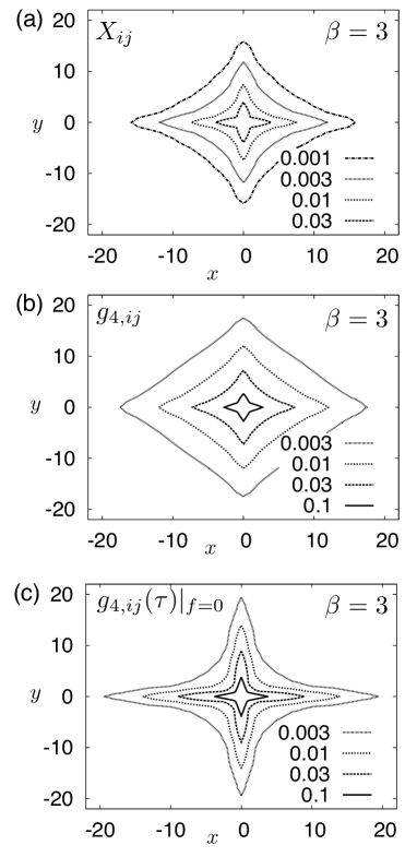
Figure 4: Real-space correlations in the SPM. (a) The correlation function $X_{ij}$ evaluated at $f=f^{*}$, in the long-time limit. The co-ordinates $x$ and $y$ give the position of spin $j$ relative to spin $i$. (b) The four-point susceptibility $g_{4,ij}$ at $f=f^{*}$ and long times. (c) The four-point susceptibility at $f=0$, evaluated at the bulk relaxation time $\tau$. The scales are the same in all plots, indicating that all correlations operate over similar length scales.

In Fig. 4, we show the behaviour of $g_{4,ij}$ and $X_{ij}$ for $f=f^{*}$ and a representative temperature $\beta=3$. We compare these correlations with the behaviour of $g_{4,ij}(t)$ measured at $f=0$ and $t=\tau$, for the same temperature. In all cases, the correlations seem to operate over a similar lengthscale (the same linear scale is used for all panels). The correlation functions are all strongly anisotropic, although we observe slightly different angular dependences in each case.

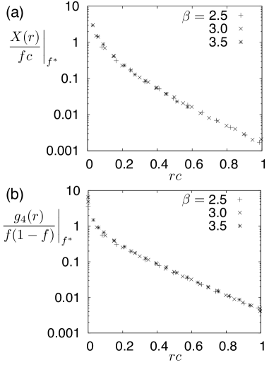
Figure 5: Circular averaged correlation functions in the SPM evaluated at $f=f^{*}$ and plotted to illustrate their scaling with temperature. (a) Circular average of $X_{ij}$. (b) Circular average of $g_{4,ij}$. In both cases the relevant length scales scale as $\xi\sim c^{-1}$. At the lower temperatures we show data points are only for those $r$ and $\beta$ where numerical uncertainties are smaller than or comparable to symbol sizes.

The dominance of a single lengthscale in this problem may be seen from Fig. 5 where we show circular averages of these correlation functions, plotted as a function of the scaling variable $rc$. It was shown in Ref. Jack et al. (2005) that dynamical four-point correlations at $f=0$ and $t=\tau$ collapse as a function of this scaling variable. Here we show that the same behaviour holds for $X_{ij}$ and $g_{4,ij}$ evaluated at $f^{*}$.

To describe the scaling behaviour of correlation functions near $f^{*}$ in the SPM, we make an ansatz for the circular averaged three-point function $X(r)$:

$$X(r)|_{f^{*}}\approx cf^{*}G_{X}(rc).$$ (14)

The choice of scaling variable $rc$ indicates that the dominant correlation length in the system scales as $\xi\sim c^{-1}$. To understand the prefactor $cf^{*}$, note that the ratio $X_{ij}/f$ quantifies the effect of freezing spin $j$ on the autocorrelation function at site $i$. Thus, if each frozen spin has an $O(1)$ effect then one would expect $X(r)\approx fG(r)$, which explains the presence of $f^{*}$ as a prefactor in Eq. (14). The extra prefactor of $c$ in Eq. (14) has two possible interpretations, which are hard to discriminate on the basis of our numerical results. First, if the correlation function $X(x,y)$ is largest near the lattice axis, and if these on-axis correlations are $O(1)$ and dominate the circular average then one arrives at $X(r)/f\approx c\,G_{X}(r)$, as in the case of the static function $g_{\mathrm{s}}(r)$. However, a second explanation could be the presence of off-axis correlations of strength $O(c)$, which would lead to the same prefactor $c$ in Eq. (14).

Our ansatz for the low-temperature scaling of of $g_{4}$ is

$$\left.g_{4}(r)\right|_{f^{*}}\approx f^{*}(1-f^{*})G_{4}(rc).$$ (15)

Again, the scaling variable $rc$ indicates that the correlation length scales as $\xi\sim c^{-1}$. In Fig. 5, we plot $g_{4}/[f^{*}(1-f^{*})]$ as a function of the scaled variable $rc$, a procedure which nicely collapses our data. The prefactor $(1-f^{*})$ is irrelevant for the purpose of scaling in the low temperature limit. However, it is natural from a physical point of view because $g_{4,ii}\propto(1-f)$, and we do find that it improves the data collapse in the studied range of temperatures. The physical interpretation of the prefactor $f^{*}$ in Eq. (15) is not immediately clear. We note that Eqs. (14) and (15) are together consistent with Eq. (10), which holds if the correlations of the $a_{i}$ are directly attributable to individual frozen spins $f_{j}$. More support for this can be obtained through a direct numerical evaluation of the right hand side of Eq. (10) which has the same dependence on $ij$ as $g_{4,ij}$, but is smaller by factor close to $5$, independently of the temperature. As a result, $\chi_{4}$ and its bound $\Delta\chi_{4}$ scale in the same way, but differ by a prefactor.

To conclude, we have shown robust evidence that $g_{4,ij}$ and $X_{ij}$ in the SPM are both controlled by the same lengthscale $\xi\sim(1/c)$. The scaling of the prefactors in these correlations is less clear, but Eqs. (14) and (15) are consistent with our numerical data. Assuming that these results do hold, we arrive at the following scaling behaviours for the susceptibilities:

$$\frac{\partial q}{\partial f}\bigg{|}_{f^{*}}\sim c^{-1},\qquad\chi_{4}|_{f^{*}}\sim\Delta\chi_{4}|_{f^{*}}\sim c^{-2}f^{*}.$$ (16)

We recall that dynamical correlations $g_{4}(r,t)|_{f=0}$ at $t=\tau$ are controlled by the same lengthscale $\xi\sim(1/c)$, but that $\chi_{4}(t=\tau)|_{f=0}\sim c^{-1}$ due to the strong anisotropy of the correlation function. Combined with the super-Arrhenius growth of the relaxation time shown in Fig. 1f, this difference in the scaling of $\chi_{4}$ emphasizes that the relaxation near $f^{*}$ is qualitatively different from bulk relaxation at $f=0$, even if the same lengthscale appears in both cases. In particular, the susceptibility $\chi_{4}$ at $f^{*}$ grows more quickly on cooling than the bulk $\chi_{4}$, consistent with the observation that relaxation is slower and more co-operative. In this respect increasing $f^{*}$ is similar to reducing the temperature. However, in contrast to decreasing $T$, there is no evidence for an increasing length scale as $f$ is increased.

IV.4 TPM: Real-space scaling at $f=f^{*}$

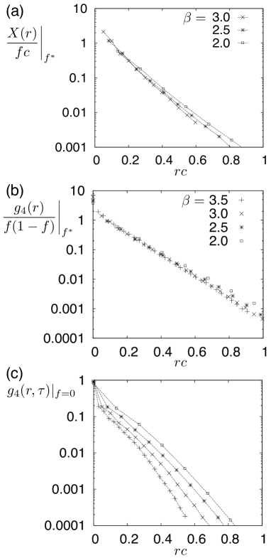
Figure 6: Circular-averaged correlations in the TPM. (a) Circular average of $X_{ij}$ at $f^{*}$, showing a length scale $\xi\sim c^{-1}$. (b) Circular average of $g_{4,ij}$ at $f^{*}$, showing a similar length scale $\xi\sim c^{-1}$. (c) Circular average of $g_{4,ij}(t)$ evaluated at $f=0$ and $t=\tau$. This correlation function clearly has a different scaling to those evaluated at $f^{*}$: it was shown in Jack and Garrahan (2005) that $\xi\sim c^{-1/d_{\mathrm{f}}}$ in this case.

For the triangular plaquette model, the isotropic images shown in Fig. 3 lead us to compute circularly averaged correlation functions directly. The results are presented in Fig. 6, showing scaling with temperature. We find that our data are most consistent with

$$X(r)|_{f^{*}}\approx cf^{*}G_{X\mathrm{T}}(rc),$$ (17)

and

$$g_{4}(r)|_{f^{*}}\approx f^{*}(1-f^{*})G_{4\mathrm{T}}(rc).$$ (18)

The most striking feature of Eqs. (17) and (18) is that the scaling variable $rc$ is the same as that found in the SPM. This suggests that correlations at $f^{*}$ extend over a length which scales as $\xi\sim 1/c$. This is surprising because the point-to-set length for the TPM at $f=0$ does not scale as $c^{-1}$, nor does the dynamic correlation length. For dynamical correlations at $f=0$ and $t=\tau$ then it is known Jack and Garrahan (2005) that $g_{4}(r,\tau)|_{f=0}\approx G_{4\mathrm{T}}(rc^{1/d_{\mathrm{f}}})$, such that both static and dynamic lengths scale as $\xi(f=0)\sim c^{-1/d_{\mathrm{f}}}\sim c^{-0.631}$. In Fig. 6c, we show that these two scaling forms can be clearly differentiated over the temperature range shown, since $g_{4}(r)|_{f=0}$ does not collapse as a function of $rc$, as expected. It is therefore clear that a new lengthscale $\xi\sim c^{-1}$ appears in the TPM near $f=f^{*}$, which is longer than any static or dynamic correlation length found previously for the bulk at $f=0$.

As in the SPM, the physical interpretation of the scaling prefactors in Eqs. (17) and (18) is not clear. The scaling laws we have proposed indicate that the bound $\Delta\chi_{4}$ scales in the same way as $\chi_{4}$, although $\Delta\chi_{4}$ is significantly smaller than $\chi_{4}$ in the TPM. We also note that while the scaling forms in Eqs. (17) and (18) in the TPM are the same as in Eqs. (14) and (15) in the SPM, we do not see any a priori reason for this result. In particular, the spatial structure of the correlations are quite different in both cases.

While the appearance of a new lengthscale near $f^{*}$ makes the TPM different from the SPM, we emphasize that the relaxation mechanism changes qualitatively near $f^{*}$ in both models. In the SPM, this appears as a larger relaxation time and a larger susceptibility without any increase in the length; in the TPM the lengthscale, time scale and susceptibilities are all different from their values at $f=0$.

V Square plaquette model: Weak and strong pinning

We have discussed the scaling of length and time scales at $f^{*}$, as temperature is reduced. In this section, we consider how $f^{*}$ depends on temperature. We focus on the SPM for which analytic calculations provide useful insight.

V.1 Small-$f$ limit

We concentrate on the behaviour of the correlation function $X_{ij}$. We define a parameter $\mu$ by $f=(1+\mathrm{e}^{\mu})^{-1}$ so that the limit of small $f$ is equivalent to a limit of small $\mathrm{e}^{-\mu}$. The correlation function $X_{ij}$ has a series expansion in powers of $\mathrm{e}^{-\mu}$ given by

$$X_{ij}=\frac{1}{Z_{\mathrm{f}}}\left[\langle a_{i}f_{j}\rangle_{0}+\mathrm{e}^{-\mu}\sum_{k}\langle a_{i}f_{j}\rangle_{k}\right.\\ +\left.\mathrm{e}^{-2\mu}\sum_{k<l}\langle a_{i}f_{j}\rangle_{kl}+O(\mathrm{e}^{-3\mu})\right]-qf(1-f),$$ (19)

where $Z_{\mathrm{f}}=(1+\mathrm{e}^{-\mu})^{V}$ and $\langle\cdots\rangle_{kl\dots}$ is an average in a system where spins $(k,l,\dots)$ are pinned and all other spins are mobile (unpinned). For details, see Appendix A, particularly Eq. (31). The factor of $q$ in Eq. (19) must be obtained by a separate series expansion over $f$.

Figure 7: Two diagrams representing contributions to $X_{ij}$ in the SPM, at order $f^{3}$. The white circle represents spin $i$, the grey circle spin $j$, and the positions of spins $klm$ are to be summed, subject to the constraint that $j$ is equal to one of $klm$. (a) Leading contribution to $X(x,y)$, assuming $x,y>0$. (b) Leading contribution to $X(x,0)$: summing over the positions of spins $l$ and $m$ corresponds to a sum over the dimension $y^{\prime}$.

Assuming $i\neq j$, symmetries of the SPM imply that the first non-zero term in the expansion is at third order,

$$\mathrm{e}^{-3\mu}\sum_{k<l<m}\langle a_{i}f_{j}\rangle_{klm}.$$ (20)

The factor $f_{j}$ means that the average is zero unless $j$ is equal to one of $k$, $l$, or $m$. As shown in Fig. 7, the correlations may be calculated in a diagrammatic expansion. Spin $i$ is shown as a white circle and has a fixed position. Spin $j$ is shown as a grey circle: its position is fixed, and we also have the constraint that one of the frozen spins $k$, $l$, or $m$ coincides with $j$. Equation (19) shows that we must sum over the positions of the remaining frozen spins: these spins are shown as black circles. To evaluate the contribution of each diagram to $X_{ij}$, we use Eq. (32) which shows how to evaluate expectation values in the presence of a fixed set of frozen spins. For the SPM, $\langle a_{i}f_{j}\rangle_{klm}$ is non-zero only if spins $iklm$ lie on the four vertices of a rectangle. If the rectangle is of size $x\times y$ then Eq. (32) yields $\langle a_{i}f_{j}\rangle_{klm}=\tanh(\beta/2)^{2xy}$. (The denominator in (32) has a trivial value $2^{-3}$ in this case, because all configurations of the frozen spins are equally likely and they all have equivalent effects on spin $i$.)

The leading order behaviour of $X_{ij}$ stems from two distinct cases, as shown in Fig. 7. If spins $i$ and $j$ are in the same row of the square lattice, with spacing $x$, then we fix $k=j$ and we sum over all sites $l$ and $m$ such that the sites $iklm$ form a rectangle. For a rectangle of size $x\times y^{\prime}$ then Eq. (32) yields $\langle a_{i}f_{j}\rangle_{klm}=\tanh(\beta/2)^{2xy^{\prime}}$. Summing over the positions of spins $l$ and $m$, one obtains a geometric series and the result is, for $x\neq 0$:

$$X(x,0)=f^{3}\frac{\tanh(\beta/2)^{2|x|}}{1-\tanh(\beta/2)^{2|x|}}+O(f^{4})$$ (21)

where we have defined $X(x,y)=X_{ij}$, evaluated for spins $i$ and $j$ that are separated by a vector $(x,y)$. A similar analysis applies if spins $i$ and $j$ are in the same column of the lattice, yielding $X(0,y)=X(y,0)$.

However, if spins $i$ and $j$ are in different rows and columns then we fix $l=j$ and we sum over sites $k$ and $m$ such that sites $iklm$ still form a rectangle. There is only one choice for $k$ and $m$ in this case, as shown in Fig. 7b. If the vector from site $i$ to site $j$ is $(x,y)$ then the resulting rectangle is $x\times y$ in size and, again, $\langle a_{i}f_{j}\rangle_{klm}=\tanh(\beta/2)^{2xy}$ so that, for $x,y\neq 0$,

$$X(x,y)=f^{3}\tanh(\beta/2)^{2|xy|}+O(f^{4}).$$ (22)

Collecting all these results and summing over the volume, Eq. (8), one finally obtains the leading order behaviour of the three-point susceptibility, namely

$$\frac{\partial q}{\partial f}=12A_{c}(T)f^{2}+O(f^{3}),$$ (23)

where

$$A_{c}(T)=\sum_{x=1}^{\infty}\frac{\tanh(\beta/2)^{2x}}{1-\tanh(\beta/2)^{2x}}\simeq\frac{\mathrm{e}^{\beta}}{4}[\beta+O(1)].$$ (24)

The final approximate equality holds for small $c$ (i.e., at low temperature) and follows because $\sum_{k}(1-\delta)^{k}/(1-(1-\delta)^{k})\approx(1/\delta)[\log(1/\delta)+O(1)]$ as $\delta\to 0$. In Fig. 8a we show that the result in Eq. (23) holds very well for small values of $f\sqrt{A_{c}}$, but breaks down for larger $f$, where higher order terms in the expansion also contribute, as discussed below.

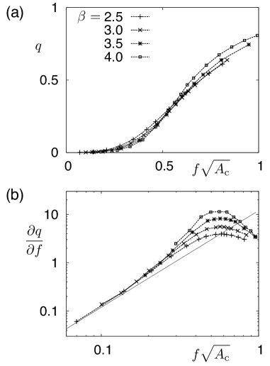
Figure 8: Plots of $q$ and $\partial q/\partial f$ for the SPM, as a function of the scaling variable $f\sqrt{A_{c}}$. (a) Plot of the overlap $q$ indicating that $f^{*}\sim A_{c}^{-1/2}$. (b) Slight change in data. The susceptibility $\partial q/\partial f$ is maximal near $f^{*}$. The straight line is the theoretical result (23) for the small-$f$ limit. This approximation applies only when $f\sqrt{A_{c}}\ll 1$ and does not capture the peak in $\partial q/\partial f$ near $f^{*}$.

The physical interpretation of this small-$f$ result is that adding one extra frozen spin $j$ affects the autocorrelation $a_{i}$ over an area of linear size $\xi\sim c^{-1}$, but the anisotropy of correlations imply that the correlation volume is $v\sim A_{c}~{}\sim(-\ln c)/c$, much smaller than the naive assumption $v\sim\xi^{2}\sim 1/c^{2}$. The strength of the response on adding the frozen spin is small (proportional to $f^{2}$) but the lengthscale controlling $X_{ij}$ is large and independent of $f$ as $f\to 0$, and the sum in Eq. (8) is dominated by correlations close to the lattice axes.

Using Eq. (23), it is then easy to integrate $\partial q/\partial f$ to obtain the low-$f$ behaviour of the overlap,

$$q=4A_{c}f^{3}+O(f^{4}).$$ (25)

It is interesting to remark that $A_{c}=\sum_{xy(\geq 0)}g_{\mathrm{s}}(x,y)^{2}$, which highlights the fact that in the limit where the randomly frozen spins are dilute, the static overlap and susceptibilities simply capture the most trivial behaviour of the bulk system. In a supercooled liquid where two-body correlations do not vanish, one would expect the overlap to be proportional to $f$ for small-$f$, with a prefactor directly given by the pair correlation function, see Eqs. (19) and (35). It is only by going beyond the leading order in $f$ one reveals the relevant higher-order correlations responsible for amorphous order ber ; tar .

V.2 SPM: Behaviour near $f=f^{*}$

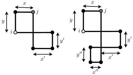
Figure 9: Two representative diagrams that contribute to $X_{ij}$ in the SPM, at order $f^{5}$ (left) and $f^{7}$ (right). The dimensions $x$ and $y$ are fixed by the positions of spins $i$ and $j$ while the primed dimensions are to be summed over. These sums yield factors of $A_{c}$ (left) and $A_{c}^{2}$ (right) in the contributions of these diagrams to $X_{ij}$.

To analyze the behaviour near $f=f^{*}$, we now consider higher-order terms in the expansion over $f$. In Fig. 9, we show two further contributions to $X_{ij}$, in the case where $i$ and $j$ are not in the same row or column. These contributions appear at order $\mathrm{e}^{-5\mu}$ and $\mathrm{e}^{-7\mu}$ in Eq. (19), respectively. For these diagrams, Eq. (32) yields $\langle a_{i}f_{j}\rangle_{kl\dots}=\tanh(\beta/2)^{2\cal A}$ where $\cal A$ is the total area of the rectangular regions enclosed by the solid lines in the diagrams. (The denominator in Eq. (32) is again trivial for these diagrams, due to symmetries of the SPM.) Summing over the positions of the frozen spins yields a factor of $A_{c}$ for each rectangle, except for the rectangle whose location is fixed by the positions of $i$ and $j$. These two diagrams therefore contribute to $X_{ij}$ as $f^{3}(f^{2}A_{c})\tanh(\beta/2)^{2xy}$ and $f^{3}(f^{2}A_{c})^{2}\tanh(\beta/2)^{2xy}$, respectively. Of course, there are various other contributions at these orders that scale in the same way. Constructing higher order diagrams similar to those in Fig. 9, one may identify a series of positive terms which are all proportional to powers of $f^{2}A_{\mathrm{c}}$. For small $c$, we expect these to be the largest terms at each order. These considerations clearly motivate the use of $f\sqrt{A_{c}}$ as a scaling variable for this expansion. Of course, if $f^{2}A_{c}$ is not a small number, then the leading terms in the small-$f$ expansion do not give a good approximation to the correlation function.

In Fig. 8 we plot $q$ and $\partial q/\partial f$ as a function of the scaling variable $f\sqrt{A_{c}(T)}$. We find that the crossover $f^{*}$, which corresponds to the maximum observed for $\partial q/\partial f$, does indeed scale as $A_{c}^{-1/2}$, so that finally

$$f^{*}(T)\approx\sqrt{\frac{-\ln c}{c}}\sim\sqrt{T}\exp\left(-\frac{1}{2T}\right).$$ (26)

This result shows that the ‘localization’ crossover at $f^{*}$ occurs along a line $f^{*}(T)$ in the $(f,T)$ phase diagram, with $f^{*}\to 0$ as $T\to 0$.

Also, the numerical data indicate that results from the small-$f$ limit such as Eq. (23) are applicable only when $f\sqrt{A_{c}}\ll 1$ and break down for $f\simeq f^{*}$. As suggested above, this strongly suggests that the maxima in $\partial q/\partial f$ and $\chi_{4}$ have their origin in non-trivial “many-body” effects that are not captured by the low-order expansion about the dilute limit.

Physically, the interpretation is that the relaxation mechanism near to $f^{*}$ is qualitatively different from the bulk relaxation at $f=0$. Perturbation theory in $f$ is not sufficient to capture this new mechanism: a non-perturbative approach would be necessary to make further analytic progress, presumably by summing infinite subsets of diagrams in the expansion of correlation functions. In this model, $f^{*}\to 0$ when $T\to 0$, indicating that the regime where perturbation theory is valid becomes vanishingly small near the glass transition of the model (which takes place at $T=0$).

VI Discussion

We have studied the effect of random pinning in the context of two finite dimensional spin models with plaquette interactions. By increasing the fraction $f$ of pinned spins at a fixed low temperature, we have discovered the existence of a temperature-dependent crossover between bulk-like relaxation at small $f<f^{*}(T)$, and a nearly localized amorphous state at large $f>f^{*}(T)$. The study of static correlation functions and susceptibilities in the presence of random pinning directly reveals the existence of growing amorphous order on cooling. This growth appears through the large lengthscales that can be measured by $X_{ij}$ and $g_{4,ij}$, and by the decreasing values $f^{*}(T)$ required to keep the system localized in a single state at lower temperature. Moreover, these measurements do not require a priori knowledge of the specific type of order that sets in at low temperature. These results therefore demonstrate that the main objective underlying the measurement of point-to-set correlation functions is fulfilled in plaquette models.

The lengthscales that we measure show scaling behaviour at low temperatures. We have emphasized that while low-order terms in the expansion over $f$ are related to static correlation functions of the bulk system at $f=0$, the length and time scales that we observe near $f=f^{*}$ are related to nonperturbative effects, and analytic calculations of lengthscales in that regime would seem to require a new approach beyond those given here.

Similarly, we have shown that length and time scales near $f^{*}$ in the plaquette models are not related in the same way as they are at $f=0$. Increasing $f$ in the SPM, we found an increasing time scale and a growing susceptibility, but without any increasing length scale. In the TPM, the length scale increases as $f$ is increased but the change in time scale is very mild, in contrast to the strong dependence observed at $f=0$ for this model.

We have also emphasized that although static and dynamic correlations are strongly enhanced near $f^{*}$ as compared to the bulk, length and time scales are finite at $f^{*}$, after taking the thermodynamic limit at any non-zero temperature. This implies that random pinning does not induce any kind of phase transition in plaquette models. It is perhaps unsurprising that these models do not exhibit an ideal glass transition in the $(f,T)$ phase diagram, since no transition occurs at finite temperature in the bulk at $f=0$ either. However, the sharp crossovers we have revealed in plaquette models represent non-trivial new results, because they have no counterparts in the bulk systems at $f=0$.

Given that neither mode-coupling theory nor RFOT theory represent accurate descriptions of plaquette models in the bulk, we do not expect these approaches to account for the effect of random pinning either. Thus, we argue that the results obtained within plaquette models provide a useful alternative reference point for interpreting simulation data for more realistic models of supercooled liquids. In particular, the absence of any phase transition at $f^{*}$ indicates that such transitions may not be generic in glassy systems with pinning.

In this respect, it is instructive to compare the results we find here with the predictions of RFOT theory cam . A central quantity in this theory is the configurational entropy, which measures the diversity of long-lived metastable states. Assuming that RFOT applies in supercooled liquids, results for model systems and renormalisation group calculations cam indicate that the configurational entropy density $s_{c}$ is well represented by

$$s_{c}(T,f)\approx s_{c}(T,0)-fY(T).$$ (27)

In 3 dimensions and above, this leads to a phase transition at $f^{*}(T)\approx Y(T)/s_{c}(T,0)$. In addition, RFOT predicts that a lengthscale $\xi_{\mathrm{PTS}}$ grows as $s_{c}(f,T)$ approaches zero, and that the relaxation mechanism at finite $f$ involves cooperative rearrangements over the lengthscale $\xi_{\mathrm{PTS}}$, much as in the bulk. We emphasise that $s_{c}$ is related to metastable states and may not be obtained from the statistics of minima on the system’s energy landscape. A precise definition of $s_{c}$ in finite-dimensional systems is slightly problematic since all metastable states have finite lifetime in that case. However, one may follow the procedure of Ref. Kurchan and Levine (2011), as long as the timescale associated with structural relaxation is well-separated from all microscopic timescales.

Turning to the plaquette models, the geometric construction of Ref. Kurchan and Levine (2011) indicates that $s_{c}$ decreases as $f$ increases, just as in RFOT theory. However, it is clear from Fig. 3 that even for $f>f^{*}$ there are sets of spins that may rearrange cooperatively, which ensures that $s_{c}$ does not vanish at $f^{*}$. Thus, while $s_{c}$ presumably decreases sharply near $f^{*}$, it does not drop to zero as predicted by Eq. (27). For supercooled liquids, RFOT predicts instead localization in a single state for $f>f^{*}$, so that if the analysis of Sec. IV were repeated for those systems then regions where cooperative motion is possible should be forbidden for $f>f^{*}$, and the light-coloured regions shown in Figs. 3 would be completely absent. In plaquette models, the existence of such regions restores a finite configurational entropy density above $f^{*}$ and the proposed phase transition is avoided. It is unclear whether such strong spatial fluctuations can be present in supercooled liquids, and whether they are properly captured by renormalization group treatments cam . This remains an area of ongoing research Cammarota et al. (2011); Castellana (2011); moo ; ang .

Thus, the plaquette models illustrate that even if the detailed predictions of RFOT do not apply, systems where configurational entropy decreases on pinning can be generically expected to exhibit increased cooperativity on increasing $f$, accompanied by growing timescales as well as growing lengths and/or growing static susceptibilities. One may also expect crossovers that sharpen and move to small $f$ on cooling. To this extent, the plaquette models are broadly consistent with published numerical results for particle models Kim (2003); Kim et al. (2011); pro ; ber ; tar , although the $f$-dependence of the relaxation time appears much weaker in the plaquette models in comparison with model liquids.

On the other hand, the most striking prediction of RFOT theory is the presence of a phase transition at finite $f^{*}$. This transition remains to be found numerically, as the behaviour for large values of $f$ and low temperatures has not been investigated in much detail so far. In the absence of such a transition, we argue that the detailed RFOT scaling predictions for length and time scales must be tested directly in order to substantiate the theory and distinguish it from a more general picture of increasing cooperativity in the presence of pinning. Testing these predictions remains however a very challenging task, especially in the absence of direct measurements of the configurational entropy. We therefore conclude that while pinning particles is an interesting new method of measuring amorphous order and its growth upon cooling, it does not necessarily resolve the central problem of how to test the fundamental assumptions of RFOT theory by practical measurements. Nevertheless, we hope future studies will investigate further the effect of random pinning in supercooled liquids, especially in the relatively unexplored regime of strong pinning.

Appendix A Correlations in systems with random pinning

In this appendix, we discuss some general results for spin systems in the presence of pinning.

A.1 Ensemble dependence of $\chi_{4}(t)$

In the systems considered here, the set of frozen spins $\bm{f}$ remains constant as the dynamics proceeds. This results in ensemble-dependent susceptibilities Berthier et al. (2005); Berthier et al. (2007a, b), such as

$$\chi_{4}(t)=\chi_{4F}(t)+\Delta\chi_{4}(t),$$ (28)

where $\chi_{4F}(t)=[(1-f)V]^{-1}\langle\delta\hat{Q}(t)^{2}\rangle_{f}$ is evaluated in a ‘restricted’ ensemble with a fixed number of frozen spins. Analysis of such ensemble-dependence can be useful for understanding how the time-independent variables (the frozen spins in this case) influence the time-dependent ones.

The difference term $\Delta\chi_{4}(t)$ may be derived as in Ref. Berthier et al. (2005) or equivalently following Ref. Berthier and Jack (2007). We write $\hat{Q}-\langle\hat{Q}\rangle=(\hat{Q}-\langle\hat{Q}\rangle_{f})+(\langle\hat{Q}\rangle_{f}-\langle\hat{Q}\rangle)$ where $\langle\cdots\rangle_{f}$ is an average with fixed $\hat{N}_{\mathrm{f}}$, as above. Substituing into Eq. (5), we note that if the restricted ensemble has $\hat{N}_{\mathrm{f}}\approx fV$ frozen spins then $\langle\hat{Q}\rangle_{f}-\langle\hat{Q}\rangle\approx V^{-1}(\partial\langle\hat{Q}\rangle/\partial f)(\hat{N}_{\mathrm{f}}-fV)$ which gives $\langle\delta\hat{Q}(t)^{2}\rangle=\langle\delta\hat{Q}(t)^{2}\rangle_{f}+V^{-2}(\partial\langle\hat{Q}\rangle/\partial f)^{2}\langle(\delta\hat{N}_{\mathrm{f}})^{2}\rangle$ (the equality is exact in the limit of large system size $V$, since the fluctuations of $\hat{N}_{\mathrm{f}}$ are small in that case). Noting that $\langle(\delta\hat{N}_{\mathrm{f}})^{2}\rangle=Vf(1-f)$ and $\partial\langle\hat{Q}\rangle/\partial f=V[(1-f)\partial C(t)/\partial f-C(t)]$ then the result (9) follows.

Since $\chi_{4F}(t)$ and $\Delta\chi_{4}(t)$ are both non-negative then $\chi_{4}(t)\geq\Delta\chi_{4}(t)$. If this bound is saturated, this means that the correlations between the $a_{i}$ are directly attributable to the influence of individual $f_{j}$. In particular, a sufficient condition for $\chi_{4}(t)=\Delta\chi_{4}(t)$ is that for a fixed choice $\bm{f}$ of frozen spins, the autocorrelations $a_{i}$ are all independent and respond linearly to the $f_{j}$, so that $\langle a_{i}(t)\rangle_{\bm{f}}=\langle a_{i}(t)\rangle_{0}+\sum_{k}f_{k}U_{ik}(t)$ where $U_{ik}(t)=X_{ik}(t)/[f(1-f)]$ is assumed independent of $f$. Physically, this condition means that the site-to-site fluctuations of the $a_{i}$ depend only on the frozen spins, and the effect of each frozen spin is independent.

In addition, independence of the $\langle a_{i}\rangle_{\bm{f}}$ means that $\langle a_{i}a_{j}\rangle_{\bm{f}}=\langle a_{i}\rangle_{\bm{f}}\langle a_{j}\rangle_{\bm{f}}$. Following Ref. Krakoviack (2010) we use an overbar to indicate the average over $\bm{f}$, so the definition of the four-point function is $g_{4,ij}=\overline{\langle a_{i}a_{j}\rangle_{\bm{f}}}-\overline{\langle a_{i}\rangle_{\bm{f}}}^{2}$. Hence, $g_{4,ij}=\sum_{kk^{\prime}}[\overline{f_{k}f_{k^{\prime}}}-f^{2}]U_{ik}U_{jk^{\prime}}$, and since the frozen spins are chosen independently one has $\overline{f_{k}f_{k^{\prime}}}-f^{2}=f(1-f)\delta_{kk^{\prime}}$. The resulting expression for $g_{4,ij}$ is given in Eq. (10) of the main text, where $g_{4,ij}$ appears as a convolution of $X_{ij}$ with itself.

We note that for Ising spin variables $s_{i}$, it is not possible to satisfy $\langle a_{i}a_{j}\rangle_{\bm{f}}=\langle a_{i}\rangle\langle a_{j}\rangle_{\bm{f}}$ in the case $i=j$. However, assuming that $\chi_{4}$ is dominated by collective behaviour and not single-site fluctuations, one still expects Eq. (10) to hold as an approximate equality if the $a_{i}$ are primarily determined by a linear response to the $f_{i}$.

A.2 Long time limit

As discussed in Sec. III, long-time limits of correlation functions in systems with pinned spins are static (thermodynamic) quantities and can be calculated within equilibrium statistical mechanics. The analysis is similar to that of Krakoviack Krakoviack (2010) for particle systems.

We write spin configurations as $\bm{s}=(s_{1},\dots,s_{V})$ and choices of frozen spins as $\bm{f}=(f_{1},\dots,f_{V})$. The distribution of the initial (reference) configuration $\bm{s}^{\mathrm{A}}$ is $P_{1}(\bm{s}^{\mathrm{A}})=\mathrm{e}^{-\beta E(\bm{s}^{\mathrm{A}})}/Z_{1}$ where $E(\bm{s}^{\mathrm{A}})$ is the energy of configuration $\bm{s}^{\mathrm{A}}$ and the partition function $Z_{1}$ enforces normalisation. The $f_{i}$ are all independent with $\langle f_{i}\rangle=f$ and so their distribution is $P_{\mathrm{f}}(\bm{f})=\mathrm{e}^{-\mu\sum_{i}f_{i}}/Z_{\mathrm{f}}$ where $\mu$ is defined through $f=(1+\mathrm{e}^{\mu})^{-1}$ and $Z_{\mathrm{f}}$ is a normalisation constant. We denote the number of frozen spins by $\hat{N}_{\mathrm{f}}=\sum_{i}f_{i}$, noting that $\hat{N}_{\mathrm{f}}+\hat{N}_{\mathrm{m}}=V$.

In the long-time limit, and for fixed $\bm{s}^{\mathrm{A}}$ and $\bm{f}$, the final configuration $\bm{s}^{\mathrm{B}}$ has probability distribution

$$P_{2}(\bm{s}^{\mathrm{B}}|\bm{f},\bm{s}^{\mathrm{A}})=\frac{1}{Z_{\mathrm{B}}(\bm{f},\bm{s}^{\mathrm{A}})}\mathrm{e}^{-\beta E(\bm{s}^{\mathrm{B}})}\prod_{i}[(1-f_{i})+f_{i}\delta_{s^{\mathrm{A}}_{i},s^{\mathrm{B}}_{i}}],$$ (29)

where $Z_{\mathrm{B}}(\bm{f},\bm{s}^{\mathrm{A}})$ is a normalisation factor, defined so that $\sum_{\bm{s}^{\mathrm{B}}}P_{2}(\bm{s}^{\mathrm{B}}|\bm{f},\bm{s}^{\mathrm{A}})=1$. Thus, in the long-time limit, averages $\langle\cdots\rangle$ are taken with respect to the distribution

$$P(\bm{f},\bm{s}^{\mathrm{A}},\bm{s}^{\mathrm{B}})=P_{\mathrm{f}}(\bm{f})P_{1}(\bm{s}^{\mathrm{A}})P_{2}(\bm{s}^{\mathrm{B}}|\bm{f},\bm{s}^{\mathrm{A}}).$$ (30)

It may be shown that this distribution is invariant under $\bm{s}^{\mathrm{A}}\leftrightarrow\bm{s}^{\mathrm{B}}$. In particular, this means that the marginal distribution of $\bm{s}^{\mathrm{B}}$ is equal to the Boltzmann distribution $P_{1}(\bm{s}^{\mathrm{B}})$. Physically, this means that structural averages and correlation functions are unaffected by the pinning. Long-time correlations between the $f_{i}$ and the $a_{i}$ may be calculated as averages with respect to the distribution (30), identifying $a_{i}=(1-f_{i})s^{\mathrm{A}}_{i}s^{\mathrm{B}}_{i}$.

A.3 Small-$f$ limit

Correlation functions between the $a_{i}$ and the $f_{i}$ in the long-time limit may be calculated in an expansion about $f=0$. The idea is simply to collect together configurations $\bm{f}$ with exactly $0,1,2,\dots$ frozen spins. Formally, one expands $P_{\mathrm{f}}(\bm{f})$ in Eq. (30) over $\mathrm{e}^{-\mu}$, so that for any observable $Y$,

$$\langle Y\rangle=\frac{1}{Z_{\mathrm{f}}}\left[\langle Y\rangle_{0}+\mathrm{e}^{-\mu}\sum_{j}\langle Y\rangle_{j}+\mathrm{e}^{-2\mu}\sum_{j<k}\langle Y\rangle_{jk}+\dots\right]$$ (31)

where $\langle Y\rangle_{jkl\dots}$ is an average over configurations $A$ and $B$, given that spins $jkl\dots$ are frozen and all other spins are unfrozen. (The average $\langle Y\rangle_{0}$ is taken without any frozen spins, so that $A$ and $B$ are independent configurations from the Boltzmann distribution and averages factorise as $\langle f_{1}(\bm{s}^{A})f_{2}(\bm{s}^{B})\rangle_{0}=\langle f_{1}(\bm{s}^{A})\rangle_{0}\langle f_{2}(\bm{s}^{B})\rangle_{0}$.)

To make progress, the key step is to write the individual expectation values in Eq. (31) as correlations with respect to the distribution $P_{1}(\bm{s}^{A})P_{1}(\bm{s}^{B})$, in which case configurations $A$ and $B$ are independently chosen configurations from thermal equilibrium (at $f=0$). We write $\langle\cdots\rangle_{0}$ for averages with respect to this distribution. Using Eq. (30), the general result is

$$\langle Y\rangle_{k_{1}k_{2}\dots k_{p}}=\left\langle Y|_{\bm{f}}\cdot\frac{2^{-p}\prod_{r=1}^{p}(1+s^{A}_{k_{r}}s^{B}_{k_{r}})}{Z_{B}(\bm{f},s^{A})}\right\rangle_{0},$$ (32)

where the notation $Y|_{\bm{f}}$ indicates that any $f$-dependence of $Y|_{\bm{f}}$ has been accounted for by substituting the specific set of frozen spins $k_{1}\dots k_{p}$. For example if $Y=a_{i}f_{j}$ as in the main text then $Y|_{\bm{f}}=a_{i}\sum_{r=1}^{p}\delta_{j,k_{r}}$ since $Y=0$ unless $f_{j}=1$. To obtain (32) we used $\delta_{ss^{\prime}}=\frac{1}{2}(1+ss^{\prime})$ for Ising spins $s$, $s^{\prime}$, and we also have that

$$Z_{B}(\bm{f},s^{A})=2^{-p}\left\langle\prod_{r=1}^{p}(1+s^{A}_{k_{r}}s_{k_{r}})\right\rangle_{s},$$ (33)

where the average is taken over the spins $s$, i.e., $\langle\cdots\rangle_{s}=\sum_{\bm{s}}(\cdots)\mathrm{e}^{-E(\bm{s})/T}/Z_{1}$.

For example, Eq. (31) can be used to calculate $q=\langle a_{i}\rangle$, leading to

$$q=\langle s_{i}\rangle_{0}^{2}+\mathrm{e}^{-\mu}\left[\sum_{j(\neq i)}\left\langle s_{i}^{A}s_{i}^{B}\frac{1+s_{j}^{A}s_{j}^{B}}{1+s_{j}^{A}\langle s_{j}\rangle_{0}}\right\rangle_{0}-V\langle s_{i}\rangle_{0}^{2}\right]\\ +O(\mathrm{e}^{-2\mu}),$$ (34)

where we used $Z_{\mathrm{f}}=(1+\mathrm{e}^{-\mu})^{V}$ and we assumed that averages are translationally invariant, $\langle s_{i}\rangle_{0}=\langle s_{j}\rangle_{0}$ etc.

If the system has inversion symmetry so that $\langle s_{i}\rangle_{0}=0$ then the denominator in Eq. (34) is trivial and the average may be evaluated directly. Physically, the denominator accounts for the fact that the autocorrelation $\langle a_{i}\rangle_{\bm{f}}$ depends on the state of $s_{i}$ in the reference configuration $\bm{s}^{A}$, and the different values of $s_{i}^{A}$ may not be equally likely. In the symmetric case, both values of $s_{i}^{A}$ are equally likely so the denominator has a trivial value.

To make progress with the general case, note that $s_{i}=\pm 1$ which means that that for any function $F(s)$ then $F(s)=\frac{1}{2}(1+s)f(1)+\frac{1}{2}(1-s)f(-1)$ and hence (for any $x$), $1/(1+xs_{i})=(1-xs_{i})/(1-x^{2})$. The result is that

$$q=\langle s_{i}\rangle_{0}^{2}+f\sum_{j(\neq i)}\frac{\langle\delta s_{i}\delta s_{j}\rangle_{0}^{2}}{1-\langle s_{j}\rangle_{0}^{2}}+O(f^{2}).$$ (35)

One may similarly show that

$$X_{ij}=f\frac{\langle\delta s_{i}\delta s_{j}\rangle_{0}^{2}}{1-\langle s_{j}\rangle_{0}^{2}}+O(f^{2}),$$ (36)

and summing over $j$ and integrating with respect to $f$ yields Eq. (35), via Eq. (8).

Physically, $X_{ij}/f$ is the change in the autocorrelation $\langle a_{i}\rangle$ if one restricts to an ensemble where $f_{j}=1$. If the spin system has two-point correlations of range $\xi$ then Eq. (36) shows that pinned spins influence mobile spins over a range of at least $\xi$, resulting in an $O(f)$ contribution to $q$. Of course, if two-spin correlation functions dominate the physics then the pinning procedure is redundant since the correlations may already be measured through the spin-spin correlation function. For the spin models we consider in this paper, multi-spin correlations dominate the physics, and we find that $X_{ij}$ is a useful way to reveal the relevant correlation lengths without requiring explicit measurement of multi-spin correlations.

References

- Ediger et al. (1996) M. D. Ediger, C. A. Angell, and S. R. Nagel, J. Phys. Chem. 100, 13200 (1996).
- Debenedetti and Stillinger (2001) P. G. Debenedetti and F. H. Stillinger, Nature 410, 259 (2001).
- Berthier and Biroli (2011) L. Berthier and G. Biroli, Rev. Mod. Phys. 83, 587 (2011).
- Bouchaud and Biroli (2004) J.-P. Bouchaud and G. Biroli, J. Chem. Phys. 121, 7347 (2004).
- Montanari and Semerjian (2006) A. Montanari and G. Semerjian, J. Stat. Phys. 125, 22 (2006).
- Kurchan and Levine (2011) J. Kurchan and D. Levine, J. Phys. A 44, 035001 (2011).
- Cavagna et al. (2007) A. Cavagna, T. S. Grigera, and P. Verrocchio, Phys. Rev. Lett. 98, 187801 (2007).
- Biroli et al. (2008) G. Biroli, J.-P. Bouchaud, A. Cavagna, T. S. Grigera, and P. Verrocchio, Nature Phys. 4, 771 (2008).
- Kob. et al. (2011) W. Kob., S. Roldan-Vargas, and L. Berthier, Nature Phys. (in press) (2011).
- (10) Dynamical heterogeneities in glasses, colloids, and granular media, Eds.: L. Berthier, G. Biroli, J.-P. Bouchaud, L. Cipelletti, and W. van Saarloos, (Oxford University Press, Oxford, 2011).
- (11) L. Berthier and W. Kob, Phys. Rev. E (in press); arXiv:1105.6203.
- (12) C. Cammarota and G. Biroli, arXiv:1106.5513.
- Lipowski (1997) A. Lipowski, J. Phys. A 30, 7365 (1997).
- Newman and Moore (1999) M. E. J. Newman and C. Moore, Phys. Rev. E 60, 5068 (1999).
- Garrahan (2002) J. P. Garrahan, J. Phys.: Condens. Matt. 14, 1571 (2002).
- Jack et al. (2005) R. L. Jack, L. Berthier, and J. P. Garrahan, Phys. Rev. E 72, 016103 (2005).
- Jack and Garrahan (2005) R. L. Jack and J. P. Garrahan, J. Chem. Phys. 123, 164508 (2005).
- Buhot and Garrahan (2002) A. Buhot and J. P. Garrahan, Phys. Rev. Lett. 88, 225702 (2002).
- (19) R. L. Jack, L. Berthier and J. P. Garrahan, J. Stat. Mech. (2006), P12005.
- Sausset and Levine (2011) F. Sausset and D. Levine, Phys. Rev. Lett. 107, 045501 (2011).
- Kim (2003) K. Kim, Europhys. Lett. 61, 790 (2003).
- (22) S. Karmarkar and I. Procaccia, arXiv:1105.4053.
- (23) B. Charbonneau, P. Charbonneau, and G. Tarjus, arXiv:1108.2494.
- Kirkpatrick and Thirumalai (1987) T. R. Kirkpatrick and D. Thirumalai, Phys. Rev. B 36, 5388 (1987).
- Kirkpatrick et al. (1989) T. R. Kirkpatrick, D. Thirumalai, and P. G. Wolynes, Phys. Rev. A 40, 1045 (1989).
- Krakoviack (2011) V. Krakoviack, Phys. Rev. E 84, 050501 (2011).
- Ritort and Sollich (2003) F. Ritort and P. Sollich, Adv. Phys. 52, 219 (2003).
- Chandler and Garrahan (2010) D. Chandler and J. P. Garrahan, Ann. Rev. Phys. Chem. 61, 191 (2010).
- Garrahan and Chandler (2003) J. P. Garrahan and D. Chandler, Proc. Natl. Acad. Sci. USA 100, 9710 (2003).
- Berthier and Garrahan (2005) L. Berthier and J. P. Garrahan, J. Phys. Chem. B 109, 3578 (2005).
- Keys et al. (2011) A. S. Keys, L. O. Hedges, J. P. Garrahan, S. C. Glotzer, and D. Chandler, Phys. Rev. X 1, 021013 (2011).
- Sasa (2010) S. Sasa, J. Phys. A 43, 465002 (2010).
- Kim et al. (2011) K. Kim, K. Miyazaki, and S. Saito, J. Phys.: Condens. Matt. 23, 234123 (2011).
- Berthier et al. (2007a) L. Berthier, G. Biroli, J.-P. Bouchaud, W. Kob, K. Miyazaki, and D. R. Reichman, J. Chem. Phys. 126, 184503 (2007a).
- Berthier et al. (2007b) L. Berthier, G. Biroli, J.-P. Bouchaud, W. Kob, K. Miyazaki, and D. R. Reichman, J. Chem. Phys. 126, 184504 (2007b).
- Berthier et al. (2005) L. Berthier, G. Biroli, J. Bouchaud, L. Cipelletti, D. El Masri, D. L’Hote, F. Ladieu, and M. Pierno, Science 310, 1797 (2005).
- Krakoviack (2010) V. Krakoviack, Phys. Rev. E 82, 061501 (2010).
- Widmer-Cooper et al. (2004) A. Widmer-Cooper, P. Harrowell, and H. Fynewever, Phys. Rev. Lett. 93, 135701 (2004).
- Widmer-Cooper and Harrowell (2007) A. Widmer-Cooper and P. Harrowell, J. Chem. Phys. 126, 154503 (2007).
- Cammarota et al. (2011) C. Cammarota, G. Biroli, M. Tarzia, and G. Tarjus, Phys. Rev. Lett. 106, 115705 (2011).
- Castellana (2011) M. Castellana, EPL 95, 47014 (2011).
- (42) J. Yeo and M. A. Moore, arXiv:1111.3105.
- (43) M. C. Angelini, G. Parisi and F. Ricci-Tersenghi, arXiv:1111.6869.
- Berthier and Jack (2007) L. Berthier and R. L. Jack, Phys. Rev. E 76, 041509 (2007).