About the Yukawa model on a lattice in the quenched approximation

Abstract

The Yukawa model in the quenched approximation is expressed as a disordered statistical mechanics model on a 4-dimensional Euclidean lattice. We study this model. A particular attention is given to the singularities of the Dirac operator in the phase diagram. A careful analysis of a particular limiting case shows that finite volume effects can be huge and questions the quenched approximation. This is confirmed by a Monte-Carlo simulation in this limiting case and without the quenched approximation. We include also some results concerning the symmetries of this model.

I Introduction and model

I.1 Introduction

Since long it has been recognized that a Quantum Field Theory can be expressed as a Statistical Mechanics problem. The two areas have benefited from this proximity and many techniques developed in one context have then been used in the other zinn . The expression of quantum field theories as statistical mechanical problems has been especially useful in the context of the fundamental theory describing the interaction of quarks and gluons i.e. Quantum ChromoDynamics (QCD), where usual perturbative techniques fail. Indeed it has been found that perturbative series in any quantum field theory have a zero convergence radius and are asymptotic but never convergent zeroradius . In such situations, it is common to resort to a numerical approach based on the Feynman path integral formulation, where the system is described by a discretized action on a space-time lattice wilson .

The numerical formulation of QCD on a lattice is nowadays among the most challenging problems of numerical physics and the progress have been very important during the last decades. The methods developed in this context can also be applied to other quantum field theories rothe in situations where perturbation theory fails, for example in the investigation of binding energies. Indeed, such calculations would require the evaluation of an infinite number of contributions in a perturbative scheme.

In this paper we study the simplest fermion quantum field theory in four space-time dimensions, that is the model introduced by H. Yukawa for the nuclear interaction yukawa . The model is described in detail in reference paper1 , but since the aim of this paper is to adopt a statistical mechanics point of view, we simply sketch extremely schematically how one goes from the nuclear physics modelization to the statistical mechanics formulation.

Similar models were analyzed some time ago using the same techniques Lee , and two distinct regimes were found: for small and large values of the coupling constant the system was numerically solvable while for intermediate values it was not. In this paper we shall address in detail this issue, also found in paper1 . The same techniques have been used for a numerical study of a similar model Gerhold , where some bound on the Higgs boson mass is established based on a Yukawa coupling between quarks and the Higgs boson.

I.2 The model

The model introduced by Yukawa aimed at a description of nuclei via the exchange of massive particles in analogy with Quantum Electrodynamics, except that the particles mediating the nuclear force have to be massive in order to have a finite range interaction. Although we assume QCD is the fundamental theory of quark interactions responsible for nuclear interactions, one boson exchange models are still mandatory in the nuclear physics community.

Therefore, in the Yukawa model, nucleons and mesons are considered elementary particles –i.e. without an internal structure–, represented by local fields. The mesons are bosons represented by a complex scalar field $\phi$ while nucleons are fermions represented by a four component grassmannian Dirac spinor $\psi$. To get a statistical mechanics model one works in an Euclidean space instead of a Minkowski space, this is achieved by performing a Wick rotation montvay and the space-time is discretized into a four-dimensional hyper-cubic lattice. One possible choice for the discretized action montvay is

$$S=\frac{1}{2}\sum_{x}\left[\left(8+\mu^{2}\right)\phi_{x}^{2}-2\sum_{\nu}\phi_{x}\phi_{x+\nu}\right]+\sum_{x}\bar{\psi}_{x}D_{\rm w}\psi_{x}+g\sum_{x}\bar{\psi}_{x}\phi_{x}\psi_{x}$$ (1)

which is the sum of three terms $S=S_{\rm KG}+S_{\rm W}+S_{\rm I}$. In the first term, which is just a Klein-Gordon action for a free bosonic field, $x$ runs over the $N$ sites, $\nu$ runs over the four space-time direction, and $\mu$ is the meson mass. The second term is a bilinear in the Dirac-Wilson operator $D_{\rm w}$. It is a $4N\times 4N$ matrix, with elements

$$\left(D_{\rm w}\right)_{x\,y}=1_{4}\delta_{x,y}-\kappa\sum_{\nu}\left((1_{4}+\gamma_{\nu})\delta_{x,y-\nu}+(1_{4}-\gamma_{\nu})\delta_{x,y+\nu}\right)$$ (2)

where $1_{4}$ is a $4\times 4$ unity matrix and $\gamma_{\nu}$ are the Dirac matrices ($\bar{\psi}$ is the conjugate of $\psi$), $\kappa$ is the so-called hopping parameter related to the bare fermion mass $M=1/\kappa-8$. The coupling between the two fields is realized in the simplest way by the third term where $g$ is the coupling constant. Every dimensional quantity has been redefined in terms of the lattice spacing $a$, therefore the model depends on the three adimensionalized lattice parameters $g$, $\mu$ and $\kappa$. It depends also on the size of the lattice. In this work we use periodic boundary conditions and take the four dimension equal.

Propagators in Quantum Field Theory are expressed using Wick contractions. From the statistical mechanics point of view it amounts to computing expectation values and to combining them together. For example the elementary fermion propagator reads:

$$S(x,y)=\frac{1}{Z}\int\left[d\phi\right]\left(D(\phi)^{-1}\right)_{xy}\det\left(D(\phi)\right)e^{-S_{\rm KG}(\phi)}$$ (3)

where $x$ and $y$ are two sites of the lattice and

$$D(\phi)=D_{\rm w}+g\phi$$ (4)

is the interacting Dirac operator. $Z$ is the normalization factor of the probability distribution of the fields and it is not calculated in practice. Propagators like (3) provide a simple way of computing the renormalized mass $m$ of an interacting particle in a QFT, as

$$C(x_{4})=\sum_{x_{1},x_{2},x_{3}}S(x,0)\sim\cosh{m\left(\frac{L}{2}-x_{4}\right)}$$ (5)

where $x_{4}$ is the time coordinate. The calculation of renormalized masses is performed by producing the fields $\phi_{x}$ according to a joint probability distribution:

$$\Pi\left(\left\{\phi_{x}\right\}\right)\sim\det\left(D(\phi)\right)e^{-S_{\rm KG}(\phi)}\$$ (6)

and computing $S(x,0)$ as the average over field configurations of $\left(D(\phi)^{-1}\right)_{0y}$. Note that it implies solving a linear system, not a full inversion of the Dirac operator.

In the bosons probability distribution Eq. 6 the evaluation of the fermionic determinant is –by large– the most expensive part of the calculation. Sophisticated methods have been developed for dealing with this difficulty, as Hybrid Monte Carlo simulations hmc , but the study of the model neglecting the effect of the determinant on the weight of field configuration, called quenched approximation, deserves interest yet and will be described in some detail in the next section. Finally, let us remind that to extract physical quantities one needs to be as close as possible to a critical point so that the operator $D(\phi)$ has low modes. This implies numerical difficulties as in the vicinity of any critical point.

II The quenched approximation

The quenched approximation consists in neglecting the variation of $\det\left(D(\phi)\right)$ among the field configurations. From a physical point of view, this determinant accounts for the creation of virtual nucleon-anti-nucleon pairs, and its effect is expected to be small as long as meson mass is smaller than nucleon one. It simplifies considerably the problem since now Eq. 6 becomes

$$\mbox{Prob}\left(\left\{\phi_{x}\right\}\right)\sim\exp\left(-\frac{1}{2}\sum_{x}\left[\left(8+\mu^{2}\right)\phi_{x}^{2}-2\sum_{\mu}\phi_{x+\mu}\phi_{x}\right]\right)$$ (7)

This distribution does not anymore involve the Dirac operator and is easy to implement. Indeed the quadratic form in the exponential can be diagonalized straightforwardly, simply going to the discrete Fourier space. We note $\tilde{\phi}_{k}$ the Fourier transform of the $\phi_{x}$. The $\tilde{\phi}_{k}$ are complex and their joint probability factorizes

$$\mbox{Prob}\left(\left\{\tilde{\phi}_{k}\right\}\right)\sim\prod_{k}\exp\left(-\frac{1}{2}\frac{\left|\tilde{\phi}_{k}\right|^{2}}{\sigma_{k}^{2}}\right)$$ (8)

with $\sigma_{k}^{2}=\frac{1}{\mu^{2}+\sum_{\nu}\hat{k_{\nu}}^{2}}$ where $\hat{k_{\nu}}=2\sin\frac{k_{\nu}}{2}$ with the extra constraint $\tilde{\phi}_{k}^{\star}=\tilde{\phi}_{-k}$ in order to get real values for $\phi_{x}$. It is then simple to draw independently the real and imaginary part of each $\tilde{\phi}_{k}$ (for $k>0$) from a centered Gaussian distribution with variance $\sigma_{k}^{2}$. The partial distribution of the $\phi_{x}$ (i.e. integrating out all $\phi_{y}$ but $\phi_{x}$) is also a Gaussian with a variance $\sigma$ independent of $x$ and given by

$$\sigma^{2}(\mu)=\frac{1}{N}\sum_{k}\sigma_{k}^{2}=\frac{1}{N}\sum_{k}\frac{1}{\mu^{2}+\sum_{\nu}\hat{k_{\nu}}^{2}}$$ (9)

In summary the $\phi_{x}$ are Gaussian dependent with the same variance and the $\tilde{\phi}_{k}$ are independent with a variance depending on $k$.

It is straightforward to compute analytically the meson correlator

$$C(t) = \left\langle\sum_{x,y,z}\phi(x_{1},x_{2},x_{3},x_{4})\phi(x_{1}+x,x_{2}+y,x_{3}+z,x_{4}+t)\right\rangle$$

$$= \frac{1}{L}\sum_{k_{4}}e^{ik_{4}t}\frac{1}{\mu^{2}+\hat{k}_{4}^{2}}\sim\cosh\mu\left(\frac{L}{2}-t\right)$$

($C$ does not depend upon the $x_{\nu}$’s due to translational invariance) however when the bosons do interact, directly or through the fermions when quenched approximation is not assumed, the analytical calculation is not possible and one has to perform numerical calculation sampling the field configurations in order to get the re-normalized meson mass. In this context, three estimators of the correlator $C(t)$ are possible. For the first estimator $C_{0}(t)$ the point $(x_{0},y_{0},z_{0,},t_{0})$ is fixed and can be chosen to be the origin, for the second estimator $C_{1}(t)$ the point $(x_{0},y_{0},z_{0,},t_{0})$ runs over all the points of the time-slice $t_{0}=0$, and for the third one $C_{2}(t)$ all pairs of lattice points are considered. Obviously these three estimators give the same average as it should due to the translational invariance, but their variances are very different. In appendix B we give the three expressions of the variance corresponding to the three estimators. We see that only $C_{2}(t)$ is self-averaging. For the first estimator the variance diverges with the size of the lattice, while for the second it goes to a finite value. It means that only with the third estimator larger sizes imply less configurations in the average. Consequently for the case of interacting bosons, in the unquenched calculation for example, the third estimator $C_{2}$ should be considered.

III Symmetries

In this section we discuss some symmetries of the Dirac operator with Yukawa coupling Eq.4. Being associated to the action, these symmetries hold in both quenched and unquenched calculations. They are interesting per se but also useful for numerical treatment.

III.1 Symmetries holding separately on each boson configuration

Let us first note that, using the representation for the Dirac matrices montvay , the operator $J=\imath\gamma_{1}\gamma_{3}$ is an involution verifying $J\gamma_{\nu}J=\mbox{transpose}(\gamma_{\nu})$ for the four Dirac matrices $\gamma_{\nu}$. It is then straightforward to verify that

$$D=JD^{\star}J$$ (10)

where $D^{\star}$ is the complex conjugate of $D$. Let $V$ be an eigenvector of $D$ belonging to the eigenvalue $\lambda$. Introducing the complex conjugation operator $K$, the vector $W=JK(V)$ is also an eigenvector of $D$ belonging to the eigenvalue $\lambda^{\star}$. Indeed $DJK(V)=JD^{\star}K(V)=JK(DV)=JK(\lambda V)=\lambda^{\star}JK(V)$. Moreover $V$ and $W$ are orthogonal. So the eigenvalues appear in pair of conjugate values and therefore the determinant is never negative. This non-negativity property is useful to perform hybrid Monte-Carlo simulation in the unquenched calculation.

The relation Eq 10 has another useful consequence. In Eq. 3 $S(x,y)$ is a $4\times 4$ matrix where row and column are indexed by the spin at sites $x$ and $y$. To compute $S(x,y)$ one solves for the propagator $X_{\sigma}$ the four linear system with the four right hand-side (source term) $Y_{\sigma}$

$$DX_{\sigma}=Y_{\sigma}$$ (11)

corresponding to the 4 spin states $\sigma=0,1,2,3$. The $4\times 4$ matrix $S(x,y)$ is obtained selecting the proper elements of the four vectors $X_{\sigma}$. We will show a relation between $X_{1}$ and $X_{2}$, obviously this relation hods also between $X_{3}$ and $X_{4}$. Indeed it is readily verified, using sing Eq. 10 , that $D\left(\imath JK(X_{1})\right)=Y_{2}$, in other words

$$X_{1}=-\imath JK(X_{2})$$ (12)

and consequently each correlation matrix, and for any field configuration, has the following form

$$S=\left(\begin{array}[]{cccc}a&b&c&d\\ -b^{\star}&a^{\star}&-d^{\star}&c^{\star}\\ e&f&g&h\\ -f^{\star}&e^{\star}&-h^{\star}&g^{\star}\end{array}\right)$$ (13)

and the trace of any of these matrix is simply $2\left(\mathcal{R}(a)+\mathcal{R}(g)\right)$. Note that this form of the correlation matrix holds also for any composite particle correlator (even using the so-called smeared source).

III.2 Symmetries holding on the average

We now show that another simplification appears when averaging the correlation matrices over the fields configurations. Let us introduce the automorphy group of the lattice, i.e. permutations $\pi$ of the sites of the lattice such that the images of two neighboring sites are also two neighboring sites. For any such permutation the two fields configurations $\phi_{x}$ and $\phi_{\pi(x)}$ have the same probability, since both the fermions and the bosons actions are invariant under the permutation $\pi$. Note that this equality also holds without the quenched approximation. Let’s denote $\pi_{1}$ the particular permutation defined by

$$\pi_{1}(x_{1},x_{2},x_{3},x_{4})=(-x_{1},x_{2},x_{3},x_{4})$$ (14)

it is clear that $\pi_{1}$ belongs to the automorphy group. We also introduce $\pi_{2}$, $\pi_{3}$ and $\pi_{4}$ corresponding respectively to $x_{2},$, $x_{3}$ and $x_{4}$. We have

$$S(x,\phi_{x})=\gamma_{5}\gamma_{k}S\left(\pi_{k}(x),\phi_{\pi_{k}(x)}\right)\gamma_{k}\gamma_{5}$$ (15)

where $x=(x_{1},x_{2},x_{3},x_{4})$ and $k=1,2,3,4$, $\gamma_{5}=\gamma_{1}\gamma_{2}\gamma_{3}\gamma_{4}$ (see ref zinn section 8.2 for the free fermion case, the extension to the Yukawa model treated in this paper is straightforward). Using this relation the 1-fermion correlation matrix, when the source is located at the origin, takes the forms

$$C(x_{4})=\sum_{x_{1},x_{2},x_{3}}S(x_{4})=\left(\begin{array}[]{cccc}c(x_{4})&0&0&0\\ 0&c(x_{4})&0&0\\ 0&0&c(L_{4}-x_{4})&0\\ 0&0&0&c(L_{4}-x_{4})\end{array}\right)$$ (16)

the precise form 16 obviously depends on the chosen representation for the Dirac matrices, but in any representation the matrix $C(t)$ depends on a single function $c(t)$ instead of 16 functions.

IV The Dirac operator spectrum in the phase space $\kappa-g$

Let us recall that the model depends on three independent parameters, $\kappa$, $g$ and $\mu$. As shown above, in the quenched approximation the probability of a $\phi_{x}$ depends only on $\mu$ and not on $\kappa$ or $g$, it is the same everywhere in the parameter space. In this section we work at constant value of $\mu\sim 0.1$

Any numerical computation of a physical quantity will imply some inversions of the Dirac operator Eq. 4. We know that this inversion will have to be performed with values of $g$ and $\kappa$ such that the linear system is difficult to invert. In practice, in some region of the $g-\kappa$ plane and for a given value of the linear sizes of the lattice, solving for $X$ the system $DX=Y$ will not be possible. Indeed, depending on the numerical method used, either the algorithm will not converge, or it will find a wrong solution. To quantify how ill conditioned the linear system is, it is customary to use the condition number. By definition a condition number measure how the solution of the system changes when the RHS term changes saad . With the appropriate choice of the norms the condition number is the ratio $r=\frac{|\lambda_{a}|}{|\lambda_{i}|}$ of the largest to the smallest modulus of the eigenvalues. With this definition, and for the type of system we consider, a system can be inverted reasonably if the condition number is smaller than $100\sim 1000$. Note however that a condition number can be arbitrarily large but still the system is invertible. This is the case if the RHS of the system is in the kernel of the operator. This situation occurs with some preconditioning.

We now note that, due to the specific form of the Dirac operator Eq. 4, one has

$$D(\alpha g,\alpha\kappa;\phi_{x})-1=\alpha\left(D(g,\kappa;\phi_{x})-1\right)$$ (17)

where $1$ denotes the $4N\times 4N$ unity matrix. Since the probability of the $\phi_{x}$’s does not depend on $g$ and $\kappa$ one is lead to introduce the polar coordinates $r$ and $\theta$ of the parameter space ($g=r\cos(\theta)\;\kappa=r\sin(\theta)$. For a given value of $\theta$ the spectrum of $D$ evolves straightforwardly : the eigenvectors are then left unchanged and the eigenvalues $\lambda_{k}$ evolve according to

$$\lambda^{k}(r,\theta)=\frac{r}{r_{0}}\lambda^{k}(r_{0},\theta)+1-\frac{r}{r_{0}}$$ (18)

In a spectral decomposition of $D$, varying $r$ only changes the relative weights of the eigensubspaces. The value of $\theta$ fixes the spectrum, and the value of $r$ the relevant part of the spectrum. In general the eigenvalues are complex $\lambda^{k}=\lambda^{k}_{\rm{R}}+\imath\lambda^{k}_{\rm{I}}$. Let us give a fixed value to $\theta$ and denote the spectrum $\lambda^{k}(r)$. We choose a reference value $r_{0}$ (one can take for example $r_{0}=1$) and note $\Lambda^{k}=\lambda^{k}(r_{0})$, one has

$$\left|\lambda^{k}(r)\right|^{2}=\left(\left|\Lambda^{k}\right|^{2}-2\Lambda_{\rm{R}}^{k}+1\right)r^{2}+2\left(\Lambda_{\rm{R}}^{k}-1\right)r+1$$ (19)

So the modulus of the each eigenvalue is a parabola as a function of $r$. All these parabola intersect at the point ($r=0,\lambda=1)$. They also intersect each other at others points, and the two extremal eigenvalues change when $r$ changes(see Fig. 1). The eigenvalue labeled by $k$ will reach its smallest value

$$m_{k}=\frac{(\Lambda^{k}_{\rm I})^{2}}{|\Lambda^{k}|^{2}-2\Lambda^{k}_{\rm R}+1}$$ (20)

for $r=\frac{\Lambda^{k}_{\rm R}-1}{|\Lambda^{k}|^{2}-2\Lambda^{k}_{\rm R}+1}$. Therefore only the eigenvalues with $\Lambda^{k}_{\rm R}<1$ and $\Lambda^{k}_{\rm I}\ll 1$ give rise to a small denominator in the condition number. When $r\simeq 0$ the eigenvalue of lowest (resp. largest) modulus will be the one with the smallest (resp. largest) value of $\Lambda_{\rm R}-1$, therefore the condition number increases continuously from the value 1. In the other limit $r\gg 1$ the eigenvalue of lowest (resp. largest) modulus will be the one with the smallest (resp. largest) value of $|\Lambda^{k}|^{2}-2\Lambda_{\rm{R}}^{k}+1$, and the condition number tends to a finite value (the ratio of the two values above). In the intermediate regime, the condition number has a very complicated behavior with a lot of maxima and minima. We analyze this behavior is the next subsection for different case.

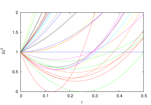
Figure 1: Evolution of the square of the modulus of some eigenvalues as a function of $r$ for the free case $g=0$ i.e. $\theta=\frac{\pi}{2}$

IV.1 case $\theta=\frac{\pi}{2}$

This correspond to $g=0$ and therefore this is the trivial case of non interacting fermions, it is included for illustrating purpose. The evolution of the spectrum of $D$ as a function of $r=\kappa$ is straightforward. Performing a discrete Fourier transform one finds that the eigenvalues are given by

$$\lambda_{k}=\left(1-2\kappa\sum_{\nu}c_{\nu}\right)\pm 2\kappa\imath\sqrt{\sum_{\nu}s_{\nu}^{2}}$$ (21)

with $c_{\nu}=\cos(k_{\nu})$ and $s_{\nu}=\sin(k_{\nu})$. Therefore the condition number behaves as

$$c(r=\kappa)=\left\{\begin{array}[]{ll}\frac{1+8\kappa}{1-8\kappa}&\kappa<\frac{1}{8}\\ \frac{1+8\kappa}{8\kappa-1}&\frac{1}{8}<\kappa<\frac{1}{6}\\ \frac{1+8\kappa}{1-4\kappa}&\frac{1}{6}<\kappa<\frac{1}{4}\\ \frac{1+8\kappa}{4\kappa-1}&\frac{1}{4}<\kappa<\frac{1}{2}\\ 1+8\kappa&\frac{1}{2}<\kappa\end{array}\right.$$

The condition number diverges at the two values $\kappa=\frac{1}{8}$ corresponding to $k=(0,0,0,0)$ and $\kappa=\frac{1}{4}$ corresponding to $k=(\frac{L_{1}}{2},0,0,0)$ (or permutation when the corresponding $L_{\nu}$ are even). The first value $\frac{1}{8}$ is the critical value, while the other is unphysical since it corresponds to a negative mass.

This is compatible with the framework introduced the introduction of this section. For example Eq 20 becomes $m_{k}=\frac{\sum{s_{\nu}^{2}}}{(\sum{c_{\nu}})2+\sum{s_{\nu}^{2}}}$. On figure Fig 1 the evolution of some eigenvalues with $r=\kappa$ is presented. One sees that for zero eigenvalues appear only for $r=\frac{1}{8}$ and $r=\frac{1}{4}$.

IV.2 case $\theta=0$

This case corresponds to $\kappa=0$ and describes infinitely heavy fermions. It is unphysical but non trivial. However it is instructive to study it from a statistical mechanics point of view, and also because if some continuity is to apply, it should not be very different from the $\theta$ small case. In that case the Dirac operator is simply diagonal and the $4\times 4$ blocs are given by

$$\left(D(\phi)\right)_{x\,y}=\left(1+g\phi_{x}\right)\delta_{xy}1_{4}$$ (23)

Obviously the eigenvalues $1+g\phi_{x}$ are all degenerated four times and real. The Eq. 19 becomes simply $(\lambda^{k}(r))^{2}=(1+r(\Lambda^{k}-1))^{2}$. Since $\lambda^{k}(r)$ is linear with $r$, for any eigenvalue $\Lambda^{k}$¡1 there will be a value of $r^{k}$ for which $\lambda(r^{k})=0$. This is the worst situation since for any fields configuration the determinant of the Dirac operator will exactly vanish $\frac{N}{2}$ times. This is illustrated on figure 1, where all the eigenvalues as a function of $g$ are shown. The two eigenvalues of largest and lowest modulus are emphasized. One clearly sees that the eigenvalue of lowest modulus vanishes for many values of $r$ (recall $r=g$ when $\kappa=0$). This situation is in contrast with the previous case $\theta=\frac{\pi}{2}$ where the eigenvalue of lowest modulus vanishes only twice (for $r=\frac{1}{8}$ and $r=\frac{1}{4}$). Here the eigenvalues are “protected” by their imaginary part.

In other words, the $\phi_{x}$ are $N$ correlated real random variables following the probability distribution Eq. 7, and we are evaluating the condition number $c(r)$ which is in that case

$$c(r;\phi)=\frac{\max\left|1+r\phi_{x}\right|}{\min\left|1+r\phi_{x}\right|}$$ (24)

Let us suppose that the $\phi_{x}$ have been sorted in ascending order. We note $\lambda_{m}$ the largest negative eigenvalue. Since $N$ is very large, we assume $m\sim\frac{N}{2}$ and there is at least one negative and one positive eigenvalue. The schema on figure Fig 2 illustrates the behavior of the spectrum of the Dirac operator for a given $\phi_{x}$ realization. Each eigenvalue varies linearly with $g$. Therefore the condition number is controlled by the eigenvalue of smallest modulus, which is a piecewise linear function of $g$. The selected eigenvalue changes each time $g$ reaches a value $g_{i}=-\frac{2}{\phi_{i}+\phi_{i+1}}$, and reaches zero for $g_{i}^{\star}=-\frac{1}{\phi_{i}}$ for $0\leq i\leq m$, which $g^{\star}_{0}<g_{0}<g^{\star}_{1}<g_{1}\cdots$. Consequently three regimes occur. Firstly when $g<g_{0}^{\star}$ the condition number is a continuous increasing function of $g$ (homographic) which diverges at $g_{0}$. Secondly in the intermediate regime $g_{0}^{\star}<g<g_{m}^{\star}$ the condition number varies extremely fast diverging $m$ times. Finally for $g_{m}^{\star}<g$ the condition number decreases homographically saturating at a finite value. This is illustrated on Fig. 2 where the extreme values $g^{\star}_{0}$ and $g^{\star}_{m}$ are indicated.

In order to perform analytical evaluation of those tree regimes we simplify the problem by choosing the fields $\phi_{x}$ independent with zero mean and a variance given by Eq. 9. It turns out that this simplification does not change substantially the average value of the eigenvalue of lowest modulus, as it is illustrated on Fig. 3. This figure shows, among other things detailed below, the two curves of the eigenvalues of lowest modulus (curves labeled $N=131072$) as a function of $r$ when the $\phi_{x}$ are independent identically distributed Gaussian variables and when they are dependent : the two curves are completely indistinguishable. Within this assumption, when the number $N$ of lattice sites increases $\phi_{m}$ goes to zero as

$$\left\langle\phi_{m}\right\rangle=-\sigma\int_{0}^{\infty}\left(1-\mbox{erf}\frac{x}{\sqrt{2}}\right)^{N}dx\sim-\sigma\sqrt{\frac{2}{\pi}}\frac{1}{N}$$ (25)

Therefore $g_{m}^{\star}\sim N$ and the third region shrinks when the lattice size increases. In other words the decreasing of the condition number for large values of the coupling constant $g$ at $\kappa=0$ is a size effect. On the other limit for small $g$, the first region $g<g_{0}^{\star}$ is delimited by the smallest field $\phi_{0}$ whose average is given by

$$\left\langle\phi_{0}\right\rangle = -\sigma\int_{0}^{\infty}\left[1-\left(\mbox{erf}\frac{x}{\sqrt{2}}\right)^{N}\right]dx$$ (26)

we see that $\left\langle\phi_{0}\right\rangle$ diverges extremely slowly with $N$. To have $\left\langle\phi_{0}\right\rangle$ of the order of $\xi$, one needs a huge lattice of $N\sim\xi\exp\frac{\xi^{2}}{2}$ sites. Therefore the first region also disappears in the thermodynamical limit. However this size effect will never be seen in an actual computation. Finally we conclude that only the second region survives the large lattice volume. Let us recall that in this region and for any fields configuration there are $m\sim\frac{N}{2}$ values of $g$ for which one eigenvalue of the Dirac operator is exactly zero.

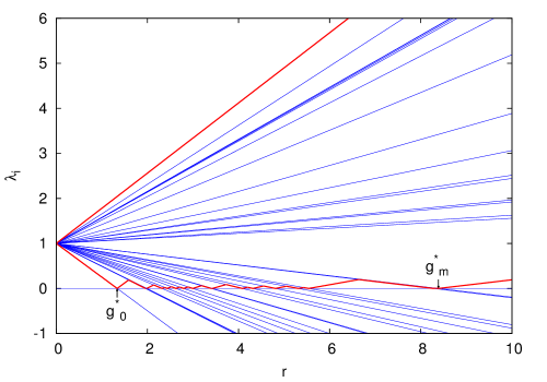
Figure 2: Schematic evolution of the modulus of the eigenvalue for one $\phi_{x}$ realization for $\kappa=0$. The modulus of the eigenvalue of largest and smallest modulus are shown in red.

In the precedent paragraph the behavior of the condition number for a given configuration of the $\phi_{x}$ has been studied. We need now to perform an average over the realization of the $\phi_{x}$. For a fixed value of $g$, different field configurations will give very different condition numbers, some of them possibly extremely large. Note however that the condition number is not a physical observable, it is only an indicator of how difficult the inversion will be. Therefore the most probable value of the condition number is maybe more sensible. From the probability distribution of the $\phi_{x}$ one can easily compute the average of the smallest and largest eigenvalues as a function of $g$. This is done in Appendix A, the result is

$$\left<|\lambda_{i}|\right> \sim \frac{1}{N}\sqrt{\frac{\pi}{2}}\sigma\,\exp\frac{1}{2\sigma^{2}}$$ (27)

$$\left<|\lambda_{a}|\right> \lesssim g\sigma\sqrt{2\ln N}$$ (28)

The eigenvalue of lowest modulus goes to zero as $\frac{1}{N}$ but the prefactor increases extremely fast when $g$ goes to zero. Since $N$ goes to infinity first, for any non zero $g$, $\left<|\lambda_{i}|\right>$ goes to zero. The eigenvalue of lowest modulus increases very slowly with $N$. This is illustrated in Fig. 3 where we show the eigenvalue of lowest modulus for several lattice volumes. On this figure and for $N=64\,32^{3}=131072$ we have plotted the result of a “genuine” simulation with dependent fields, another simulation with independent fields, a numerical integration of Eq. 31, and the approximation Eq. 27. The agreement between these four calculation is excellent. We have also plotted the eigenvalue of lowest modulus for other values of $N$ to show the size effects.

The appearance of the three regions described above can be seen in figure 4. On this figures we have plotted the average condition number $\left<\frac{|\lambda_{\rm max}|}{|\lambda_{\rm min}|}\right>$ over 8692 samples as a function of $g$. If we would have used a smaller discretization of $g$ we would have even more sharp peaks. The quantity $\frac{<|\lambda_{\rm max}|>}{<|\lambda_{\rm min}|>}$ is much smoother since $<|\lambda_{\rm min}|>$ never vanishes, and also displays the three regimes. Moreover in the quenched approximation it makes sense to consider a particular realization since the weight of a consideration does depend only on $\mu$, we therefore have plotted a typical configuration. Finally we have also plotted the average condition number without the quenched approximation : this is discussed in the next section.

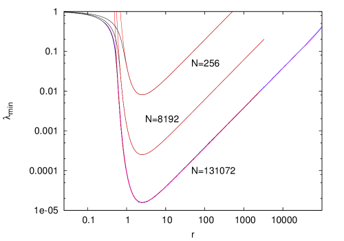
Figure 3: Smallest modulus of the eigenvalues vs $g$ for $\kappa=0$ and three values of $L$. For any value of $L$ the numerical integration (black) together with the approximation (red) Eq. 31 are shown. For the largest size $L=32\times 16^{3}$ the result of a simulation averaged over 8692 samples is also shown for both correlated $\phi_{x}$ (magenta) and uncorrelated $\phi_{x}$ (blue). Actually the curves are indistinguishable except for small $g<1$ when the approximation of the integral is not correct.

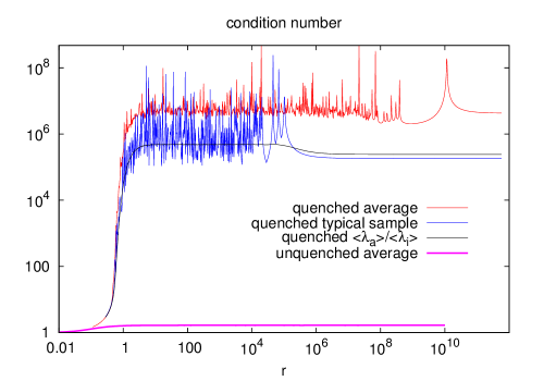
Figure 4: Condition number vs $g$ for $\kappa=0$ for a $32\times 16^{3}$ lattice. The quenched average over 8692 samples is shown in red, and a typical quenched sample is shown in blue. For comparison the ratio $\frac{|\lambda_{a}|}{|\lambda_{i}|}$ is also shown in black. The results of the unquenched Monte-Carlo simulation is the thick purple line.

In conclusion of this subsection, the size effects on this model for $\kappa=0$ appear extremely severe: for any fixed value of $g$ the occurrence of configurations with arbitrarily small eigenvalues in absolute value grows with the size. This is reminiscent of the so-called “exceptional configurations” which have been encountered in the context of quenched lattice QCD protection .

IV.3 case $0<\theta<\frac{\pi}{2}$

This region is non trivial since the Dirac operator cannot be diagonalized as in the two previous cases. Nevertheless this is where the physics takes place. As it has been done in Ref. paper1 , to perform realistic calculation one finds the critical line, and one chooses the particular point close to this line where the ratio of the renormalized masses of fermion and boson is equal to the physical one. This program has been done successfully giving consistent results for $g$ small. However for $g$ around 0.7, the linear system Eq. 11 becomes ill conditioned, preventing any conclusive result.

We have computed the condition number for a typical field configuration and the result is presented in Fig. 5. It has been shown in paper1 that for small $g$ the critical line, defined as the line where the renormalized mass of the fermion vanishes, is a parabola originating from the point $\kappa=\frac{1}{8},g=0$. We therefore expected a diverging condition number along this line. This is clearly seen on Fig. 5. When the coupling $g$ increases it enters in an ill conditioned region where the condition number shows large fluctuations. The localization of this ill conditioned region for $\kappa$ small agrees with what we have shown in Sec. IV.2. Then we can ask if this region where the condition number is small enough is not a size effect, as for the case $\kappa=0$.

We see three possible origins for this problematic region. It can be that quenched approximation is not working for those values of $g$. This seems intuitively reasonable since the determinant in Eq 6 precisely give a low weight to these configuration with a large condition number. Another possible reason could be the specific choice of the action and the discretization of the fermion. Finally there is the possibility that this a fundamental problem of the Yukawa model.

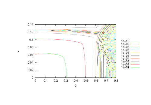
Figure 5: Iso-condition number line on a $16^{4}$ lattice.

V The $\kappa=0$ case without the quenched approximation

In this section we consider the simple case $\kappa=0$ as in the subsection sec. IV.2, but without the quenched approximation. The purpose is to illustrate on this simple case the consequence of the quenched approximation. Intuitively the determinant in the probability density Eq. 6 of the $\phi_{x}$ gives a vanishing weight to the non invertible configurations. So we can expect that the configurations to include in the sampling will not have a large condition number. But it is possible to have a large determinant, and still a small eigenvalue, for example if one eigenvalue is small and all the others are large. These configurations would have a non vanishing weight, but still a very large condition number.

The joint probability of the fields $\phi_{x}$ Eq. 6 can be written as

$$\Pi\left(\left\{\phi_{x}\right\}\right)\sim\exp\left(-\frac{1}{2}\sum_{x}\left[\left(8+\mu^{2}\right)\phi_{x}^{2}-2\sum_{\mu}\phi_{x+\mu}\phi_{x}\right]+4\ln\left|1+g\phi_{x}\right|\right)$$ (29)

Since this expression cannot be factorized we have written a simple Monte-Carlo algorithm to generate the $\phi_{x}$’s. We use the simple metropolis algorithm metropolis . The normalization factor of Eq. 6 is very difficult to compute, but the ratio of the probability of two $\phi$ configurations is very simple to compute (see Eq. 29). The Monte-Carlo method use this fact to construct a Markov chain which has the desired distribution as a fixed point. In practice, we start from a initial $\phi_{x}$ configuration, then we choose at random a site $x$ and try to change the value $\phi_{x}$ for $\phi_{x}+d\phi$ where $d\phi$ is a random number normally distributed. We accept this change with the probability $\min(1,\Delta E)$ where $E$ is the variation of the argument of the exponential in Eq. 29. We do not have a proof that this algorithm converge, the difficulty being that the number of states of the Markov chain is infinite. However for all practical purpose it works properly if one choose always as a starting distribution for a value $g$ an equilibrium distribution for a close smaller value $g-\delta g$. This indicates that the energy landscape is complicated, probably with metastable states. This naive algorithm is much simpler than the well known hybrid Monte-Carlo algorithm hmc , but it is sufficient for our purpose here. We have compare the two algorithms finding that hybrid Monte-Carlo algorithm is more efficient than the naive Monte-Carlo if the parameters are properly chosen, but they both give the same results with a good accuracy.

Before analyzing the condition number, let us look at the mean value $\left<\phi_{x}\right>$ (vacuum expectation value). Let us first recall that in the quenched approximation, due to the symmetry of Eq. 7 the average value $\left<\phi_{x}\right>$ is zero. This not the case without the unquenched approximation as seen on Fig. 6, even for small $g$. Indeed performing a $g$-expansion of Eq. 29 one finds that for any site $x$

$$\left<\phi_{x}\right>_{g}=g\sum_{y}\left<\phi_{x}\phi_{y}\right>_{g=0}+O(g^{3})=\frac{g}{\mu^{2}}+O(g^{3})$$ (30)

The insert of Fig. 6 shows the slope $\frac{1}{\mu^{2}}$ at the origin : the agreement is very good. Since the average $\left<\phi_{x}\right>$ grows with $g$, it seems likely that $\min(|1+g\phi|)$ will not easily become small. This is indeed confirmed in Fig. 7 where we have plotted the eigenvalues of minimum and maximum modulus for both the quenched and unquenched case. It is clearly seen that $\lambda_{\rm min}$ is never small. Finally the average condition number is plotted on Fig. 4 where the drastic effect of the quenched approximation is clearly seen : a reduction by six order of magnitude of the condition number. This reduction is larger with larger lattice. We conclude that there is no ill conditionned point on this $\kappa=0$ line without the quenched approximation, whereas it is everywhere ill conditionned in the quenched approximation.

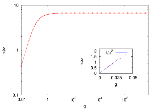
Figure 6: $<\phi>$ in an unquenched simulation on a $32\times 16^{3}$ lattice for $\kappa=0$

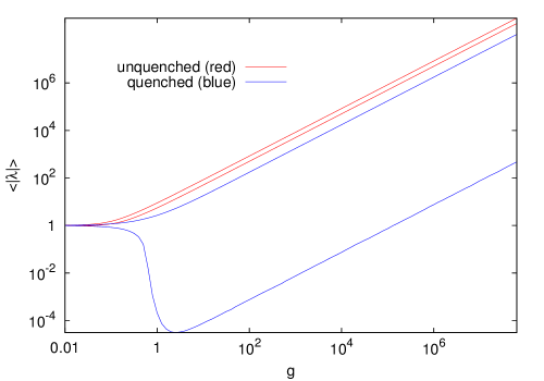
Figure 7: $\lambda_{\rm min}$ and $\lambda_{\rm max}$ in both a quenched and an unquenched simulation for $\kappa=0$ (see also Fig. 3)

VI Summary and perspectives

We have analyzed in the present paper the appearance of very small eigenvalues of Dirac operator in a Yukawa theory with Wilson fermions. The results obtained lead to the conclusion that at finite volume and within the quenched approximation, these small eigenvalues are present in an entire region of the phase space. This indicates the existence of an ill conditioned region, not just an ill conditioned line, for example the entire $\kappa=0$ line is ill conditioned in the quenched approximation. Moreover the size effects are exponentially large and consequently a numerical calculation can give apparently correct results, which would not survive the infinite volume limit. In other words it does not seem possible to determine numerically the ill conditioned region. The origin of this difficulty could be simply the choice of the discretization, or it could be the non validity of quenched approximation. This hypothesis is supported by a an unquenched calculation for $\kappa=0$, that is nowhere ill conditioned. But it could also be a problem of the Yukawa model itself. Indeed the Yukawa model is not a gauge model and there is no protection against spurious low eigenvalues like in QCD protection .

In this context we feel that the model should be studied without the quenched approximation. However a boson self coupling term $\lambda\phi^{4}$ has to be added to the Lagrangian to ensure renormalizability. This work is in progress.

Appendix A Average of extreme eigenvalues for $\kappa=0$

In this appendix we show Eq. 27 and Eq. 28. Since the $\phi_{x}$ are normally distributed with zero mean and variance given by Eq. 9 the integrated probability distribution of $|\lambda|$ is

$$F_{|\Lambda|}(|\lambda|)=\frac{1}{2}\left({\rm erf}(\frac{|\lambda|-1}{\sqrt{2}g\sigma})+{\rm erf}(\frac{|\lambda|+1}{\sqrt{2}g\sigma})\right)$$

where $\sigma$ is the variance of the $\phi_{x}$. Then from the definition of the min and after an integration by part, one gets

$$\left<|\lambda_{\rm min}|\right> = \int_{0}^{\infty}{(1-F_{|\Lambda|}(x))^{N}dx}$$ (31)

$$\left<|\lambda_{\rm max}|\right> = \int_{0}^{\infty}{1-(F_{|\Lambda|}(x))^{N}dx}$$ (32)

introducing $\phi(y)=1-F_{\sigma}(y)$ we have

$$\left\langle\lambda_{\mbox{min}}\right\rangle=\frac{1}{N}\int_{0}^{\infty}\left(\phi(\frac{y}{N})\right)^{N}dy$$

Since

$$\phi(h)=1-\sqrt{\frac{2}{\pi}}\frac{1}{\sigma}\exp-\frac{1}{2\sigma^{2}}h+O(h^{3})$$

then

$$\phi(\frac{x}{N})^{N}\rightarrow\exp\left(-x\sqrt{\frac{2}{\pi}}\frac{1}{g\sigma}e^{-\frac{1}{2g\sigma^{2}}}\right)$$

so

$$N\lambda_{\min}=\int_{0}^{\infty}\exp\left(-x\sqrt{\frac{2}{\pi}}\frac{1}{\sigma}e^{-\frac{1}{2\sigma^{2}}}\right)dx$$

yielding Eq. 25

We now study the behavior of $\lambda_{\mbox{max}}$. When $N$ is large the integrand in Eq. 32 tends to a step function equal to one for $x<x^{\star}$ and equal to zero for $x>x^{\star}$. One can estimate $x^{\star}$ as the unique zero of the second derivative of the integrand. Since $x^{\star}$ grows when $N$ grows, one can replace $x-1$ and $x+1$ by $x$ in the equation $\frac{d^{2}}{dx^{2}}F_{|\Lambda|}(x)^{N}=0$ yielding the equation

$$N=\sqrt{\frac{\pi}{2}}\frac{\left\langle\lambda_{\rm max}\right\rangle}{g\sigma}\exp\frac{1}{2}\left(\frac{\left\langle\lambda_{\rm max}\right\rangle}{g\sigma}\right)^{2}$$

from which Eq. 28 follows.

Appendix B Estimators of boson correlator

The three estimators give the same correlator

$$C(t)=\frac{1}{L}\sum_{k_{4}}\frac{1}{\mu^{2}+\hat{k}_{4}^{2}}e^{ik_{4}t}$$ (33)

However the variances are different:

$$\sigma_{0}^{2}=\left\langle C_{0}^{2}(t)\right\rangle-\left\langle C_{0}(t)\right\rangle^{2} = C^{2}(t)+A_{\mu}(L)C(t)$$

$$\sigma_{1}^{2}=\left\langle C_{1}^{2}(t)\right\rangle-\left\langle C_{1}(t)\right\rangle^{2} = C^{2}(t)+C(0)C(t)$$

$$\sigma_{2}^{2}=\left\langle C_{2}^{2}(t)\right\rangle-\left\langle C_{2}(t)\right\rangle^{2} = B_{\mu,L}(t)$$

with

$$A_{\mu}(L) = \sigma^{2}\ L^{3}$$

$$B_{\mu,L}(t) = \frac{1}{L^{2}}\sum_{k}\frac{1+e^{2\imath kt}}{\left(\mu^{2}+\hat{k_{4}^{2}}\right)^{2}}$$

where $\sigma$ is defined in the text Eq. 9. Consequently one find $\sigma_{0}^{2}$ diverges as $L^{3}$, $\sigma_{1}^{2}$ tends to a finite value and $\sigma_{2}^{2}$ goes to zero as $\frac{\alpha_{\mu}}{\sqrt{L}}$ with $\alpha_{\mu}\sim\frac{1}{\mu^{4}}\quad\mu\rightarrow 0$. Only the third estimators $C_{2}(t)$ is self-averaging.

- (1) Jean Zinn-Justin Quantum field theory and critical phenomena Oxford University Press Inc., New-york (2002)
- (2) F. J. Dyson, Phys. Rev. 85 (1952) 631
- (3) L. I. Schiff, Phys. Rev. 92 (1953) 766, K. G. Wilson, Rev. Mod. Phys. 55 (1983) 583.
- (4) H.J. Rothe, Lattice gauge theory (World Scientific Lecture Note in Physics - Vol 74 2005)
- (5) Yukawa, Proc. Math. Soc. Jpn. 17, 48 (1935).
- (6) F. de Soto , J.C. Anglès d’Auriac and J. Carbonell Eur. Phys. J. A (2011) 47
- (7) I-H. Lee, J. Shigemitsu and R. E. Shrock, Nucl. Phys. B 330 (1990) 225.
- (8) P. Gerhold and K. Jansen, JHEP 1004 (2010) 094 [arXiv:1002.4336 [hep-lat]].
- (9) I. Montvay, G. Munster, Quantum Fields on a Lattice (Cambridge University Press, 1994)
- (10) S. Duane, A.D. Keneedy, J. Pendleton, D. Roweth Phys. Lett. B195, 2 (1987)
- (11) Y. Saad Iterative method for sparse linear system Manchester University Press (2000).
- (12) R. Frezzotti Nucl.Phys.Proc.Suppl. 119 (2003)
- (13) F. de Soto, J. Carbonell, C. Roiesnel, Ph. Boucaud, J.P. Leroy, O. Pene, Nucl. Phys. B Proc. Suppl. 164 (2007) 252.
- (14) F. de Soto, J. Carbonell, C. Roiesnel, Ph. Boucaud, J.P. Leroy, O. Pene, Eur. Phys. J A31, 777 (2007); hep-lat/0610084
- (15) F. de Soto, J. Carbonell, C. Roiesnel, Ph. Boucaud, J.P. Leroy, O. Pene, Nucl. Phys. A 790 (2007) 410 ; hep-lat/0610086
- (16) N. Metropolis, A.W. Rosenbluth, M.N. Rosenbluth, A.H. Teller, A.H., E. Teller Journal of Chemical Physics 21 (1953)