An analytical solution of Shallow Water system coupled to Exner equation

Abstract

In this paper, an exact smooth solution for the equations modeling the bedload transport of sediment in Shallow Water is presented. This solution is valid for a large family of sedimentation laws which are widely used in erosion modeling such as the Grass model or those of Meyer-Peter & Müller. One of the main interest of this solution is the derivation of numerical benchmarks to valid the approximation methods. To cite this article: A. Name1, A. Name2, C. R. Acad. Sci. Paris, Ser. I 340 (2005).

Résumé Une solution analytique du système de Saint-Venant couplé à l’équation d’Exner. Ce papier présente une solution analytique pour le système modélisant le transport de sédiments par le charriage. Cette solution est valable pour une grande famille de lois sédimentaires comme le modèle de Grass ainsi que celui de Meyer-Peter & Müller. Ce résultat est utile pour la validation des schémas numériques. Pour citer cet article : A. Name1, A. Name2, C. R. Acad. Sci. Paris, Ser. I 340 (2005).

, , and

Received *****; accepted after revision +++++
Presented by

1 Introduction

Soil erosion is a consequence of the movements of sediments due to mechanical actions of flows. In the context of bedload transport, a mass conservation law, also called Exner equation [1], is used to update the bed elevation. This equation is coupled with the shallow water equations describing the overland flows (see [2] and references therein) as follows:

$$\partial_{t}h+\partial_{x}(hu)=0,$$ (1)

$$\partial_{t}(hu)+\partial_{x}(hu^{2}+gh^{2}/2)+gh\partial_{x}z_{b}=0,$$ (2)

$$\partial_{t}z_{b}+\partial_{x}q_{b}=0,$$ (3)

where $h$ is the water depth, $u$ the flow velocity, $z_{b}$ the thickness of sediment layer which can be modified by the fluid and $g$ the acceleration due to gravity. The variable $hu$ is also called water discharge and noted by $q$. Finally, $q_{b}$ is the volumetric bedload sediment transport rate. Its expressions are usually proposed for granular non-cohesive sediments and quantified empirically [3, 4, 5].

Many numerical schemes have been developed to solve system (1-3) (see [5] and references therein). The validation of such schemes by an analytical solution is a simple way to ensure their working. Nevertheless, analytical solutions are not proposed in the literature. Up to our knowledge, asymptotic solutions, derived by Hudson in [6], are in general adopted to perform some comparisons with approximated solutions. The solutions are derived for Grass model [3], i.e $q_{b}=A_{g}u^{3}$, when the interaction constant $A_{g}$ is smaller than $10^{-2}$. In this paper, we propose a non obvious analytical solution in the steady state condition of flow.

2 Solution of the equations

In order to obtain an analytic solution, we consider $q_{b}$ as a function of the dimensionless bottom shear stress $\tau^{*}_{b}$ (see [5]). By using the friction law of Darcy-Weisbach, $\tau^{*}_{b}$ is given by

$$\tau^{*}_{b}=\frac{fu^{2}}{8(s-1)gd_{s}},$$

where $f$ is the friction coefficient, $s=\rho_{s}/\rho$ the relative density of sediment in water and $d_{s}$ the diameter of sediment. The formulæ  of $q_{b}$ is usually expressed under the form

$$q_{b}=\kappa(\tau^{*}_{b}-\tau^{*}_{cr})^{p}\sqrt{(s-1)gd^{3}_{s}},$$ (4)

where $\tau^{*}_{cr}$ is the threshold for erosion, $\kappa$ an empirical coefficient and $p$ an exponent which is often fixed to $3/2$ in many applications. The expression (4) can be written in the simple form

$$q_{b}=Au_{e}^{2p},$$ (5)

where the effective velocity $u_{e}$ and the interaction coefficient $A$ are defined by

$$\left\{\begin{array}[]{l}u_{e}^{2}=u^{2}-u_{cr}^{2},\\ u_{cr}^{2}=\tau^{*}_{cr}\Big{[}\dfrac{f}{8(s-1)gd}\Big{]}^{-1},\\ A=\kappa\Big{[}\dfrac{f}{8(s-1)gd}\Big{]}^{p}\sqrt{(s-1)gd^{3}_{s}}.\end{array}\right.$$ (6)

Remark. The Grass model [3] is one of the simplest case by using $p=3/2,\leavevmode\nobreak\ \tau^{*}_{cr}=0$ and an empirical coefficient $A_{g}$ instead of $A$. The Meyer-Peter & Müler model [4] is one of the most applied by using $p=3/2,\leavevmode\nobreak\ \kappa=8,\leavevmode\nobreak\ \tau^{*}_{cr}=0.047$. The following result is valid for all models rewriting in form (5-6).

Proposition 2.1

Assume that $q_{b}$ is defined by (4). For a given uniform discharge $q$ such that $\tau^{*}_{b}>\tau^{*}_{cr}$, system (1-3) has the following analytical unsteady solution

$$\left\{\begin{array}[]{l}u^{2}_{e}=\Big{[}\dfrac{\alpha x+\beta}{A}\Big{]}^{1/p},\\ u=\sqrt{u_{e}^{2}+u_{cr}^{2}},\leavevmode\nobreak\ h=q/u,\\ z_{b}^{0}=-\dfrac{u^{3}+2gq}{2gu}+C,\\ z_{b}=-\alpha t+z_{b}^{0}.\end{array}\right.$$ (7)

where $\alpha,\leavevmode\nobreak\ \beta,\leavevmode\nobreak\ C$ are constants and $A,\leavevmode\nobreak\ u_{cr}$ are defined by (6).

Proof. We are here concerned by the smooth solution. In view of the assumption $hu=q=\text{cst}$, equations (1-3) reduce to

$$\partial_{t}h=0,$$

$$\partial_{x}(q^{2}/h)+gh\partial_{x}H=0,$$ (8)

$$\partial_{t}H+\partial_{x}q_{b}=0,$$ (9)

where $H=h+z$ is the free surface elevation. Differentiating equation (8) with respect to $t$ and then equation (9) with respect to $x$, we obtain

$$\partial_{xt}H=0,$$

$$\partial^{2}_{x}q_{b}=0.$$ (10)

Note that we can write $q_{b}=q_{b}(h,q)$ to have $\partial_{t}q_{b}=\partial_{h}q_{b}\partial_{t}h+\partial_{q}q_{b}\partial_{t}q=0$, so $q_{b}$ is not time-depending. Thank to (10), the expression of $q_{b}$ is obtained under the form

$$q_{b}=\alpha x+\beta,$$ (11)

where $\alpha$ and $\beta$ are constant. From (3), we obtain $\partial_{t}z_{b}=-\partial_{x}q_{b}=-\alpha$ to write

$$z_{b}=-\alpha t+z_{b}^{0}(x).$$ (12)

Moreover, from (5) we deduce the effective velocity as follows:

$$u_{e}^{2}=\Big{[}\dfrac{\alpha x+\beta}{A}\Big{]}^{1/p}.$$

Plugging (12) into the momentum equation (8) and using a direct calculation, we have

$$\partial_{x}z_{b}^{0}=\Big{[}\frac{q}{u^{2}}-\frac{u}{g}\Big{]}\partial_{x}u\Rightarrow z_{b}^{0}=-\frac{u^{3}+2gq}{2gu}+C$$

which concludes the proof.

Remark. As $h$ and $u$ are stationary, the initial condition of (7) is $(h,u,z_{b}^{0})$. Moreover, the solution $(h,u)$ applied to the Grass model is also an analytical solution of the Shallow Water Equations with the variable topography $z_{b}^{0}$. Concerning the shallow-water model, other solutions can be found in [7].

3 Numerical experiments

In this section, we consider the analytical solution (7) applied to the Grass model with $q=1$, $A_{g}=\alpha=\beta=0.005$ and $C=1$. A relaxation solver is applied to approximate the solution of the model. We will not give here the details of the relaxation solver (for details see [8]), but just the relaxation model for the equations (1-3). Thus, we solve the following relaxation system:

$$\left\{\begin{array}[]{l}\partial_{t}h+\partial_{x}(hu)=0,\\ \partial_{t}(hu)+\partial_{x}(hu^{2}+\pi)+gh\partial_{x}z_{b}=0,\\ \partial_{t}\pi+u\partial_{x}\pi+\frac{a^{2}}{h}\partial_{x}u=0,\\ \partial_{t}z_{b}+\partial_{x}q_{r}=0,\\ \partial_{t}q_{r}+\left(\frac{b^{2}}{h^{2}}-u^{2}\right)\partial_{x}z_{b}+2u\partial_{x}q_{r}=0,\end{array}\right.$$

that is completed with $\pi=gh^{2}/2$ and $q_{r}=q_{b}$ at the equilibrium. Figure 1 presents the numerical result with $J=500$ space cells, a CFL fix condition of $1$ and $T=7s$. We only notice little difference on the velocity, near the inflow boundary.

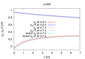
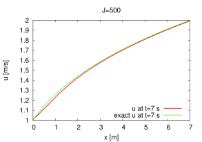
Figure 1: Comparison between the exact solution and the relaxation method for : the water height and the topography (left) and the velocity (right).

References

• [1] F. Exner. Über die wechselwirkung zwischen wasser und geschiebe in flüssen, Sitzungsber., Akad. Wissenschaften pt. IIa; 1925. Bd. 134.
• [2] M.J. Castro Díaz, E.D. Fernández-Nieto, and A.M.Ferreiro. Sediment transport models in shallow water equations and numerical approach by high order finite volume methods. Computers & Fluids, 37(3):299–316, March 2008.
• [3] A.J. Grass. Sediment transport by waves and currents. SERC London Cent. Mar. Technol, Report No. FL29, 1981.
• [4] E. Meyer-Peter and R. Müller. Formulas for bed-load transport. In 2nd meeting IAHSR, Stockholm, Sweden, pages 1–26, 1948.
• [5] S. Cordier, M.H. Le, and T. Morales de Luna. Bedload transport in shallow water models: Why splitting (may) fail, how hyperbolicity (can) help. Advances in Water Resources, 34(8):980 – 989, 2011.
• [6] J. Hudson. Numerical technics for morphodynamic modelling. PhD thesis, University of Whiteknights, 2001.
• [7] O. Delestre, C. Lucas, P.-A. Ksinant, F. Darboux, C. Laguerre, T.N.T. Vo, F. James and S. Cordier. SWASHES: a library of Shallow Water Analytic Solutions for Hydraulic and Environmental Studies (Submitted), http://arxiv.org/abs/1110.0288
• [8] E. Audusse, C. Chalons, O. Delestre, N. Goutal, M. Jodeau, J. Sainte-Marie and B. Spinewine. Sediment transport modelling : Three layer models and relaxation schemes. In preparation : CEMRACS 2011.