Quantum correlations and least disturbing local measurements

Abstract

We examine the evaluation of the minimum information loss due to an unread local measurement in mixed states of bipartite systems, for a general entropic form. Such quantity provides a measure of quantum correlations, reducing for pure states to the generalized entanglement entropy, while in the case of mixed states it vanishes just for classically correlated states with respect to the measured system, as the quantum discord. General stationary conditions are provided, together with their explicit form for general two-qubit states. Closed expressions for the minimum information loss as measured by quadratic and cubic entropies are also derived for general states of two-qubit systems. As application, we analyze the case of states with maximally mixed marginals, where a general evaluation is provided, as well as $X$ states and the mixture of two aligned states.

I Introduction

There is currently a great interest on new measures of quantum correlations for mixed states, different from the entanglement measures BDSW.96 . Quantum entanglement is essential for quantum teleportation Be.93 ; NC.00 and also for pure state quantum computation, where its increase with system size is necessary to achieve an exponential speedup over classical computation JL.03 ; Vi.03 . However, the computation model proposed by Knill and Laflamme KL.98 has shown that for mixed states, such speedup can in principle be achieved without entanglement DFC.05 . This suggests the subsistence of useful quantum correlations in some separable mixed states, which, we recall, are defined as convex mixtures of product states RF.89 . While a separable pure state is a product state, separable mixed states comprise product states, mixtures of commuting products and also mixtures of non-commuting product states. The latter can possess entangled eigenstates and give rise to non-classical capabilities.

Consequently, measures such as the quantum discord OZ.01 ; HV.01 ; Ve.03 ; ZZ.03 have recently received much attention. While coinciding with the entanglement entropy for pure states, the quantum discord is non-zero for separable mixed states of the last type, vanishing just for classically or one-way classically correlated states, i.e., states diagonal in a standard or conditional product basis. The circuit of KL.98 was in fact shown in DSC.08 to exhibit a non-negligible discord. Other measures with similar properties include the one-way information deficit Ho.05 ; SKD.11 , the geometric discord DVB.10 , based on the standard Hilbert-Schmidt norm, and the general entropic measures which we defined in RCC.10 , based on generalized entropic forms. The latter contain the two previous measures as particular cases, embedding them in a unified picture. Since they are applicable with entropic forms complying with minimum requirements, they offer, like the geometric discord, the possibility of easier evaluations, allowing at the same time to identify some universal features exhibited by all these measures RCC.10 . Related generalized measures vanishing just for full classically correlated states, like those of MV.10 and SL.08 , were also considered RCC.10 . Let us remark that important quantum capabilities of separable states with non-zero discord, and hence non-zero values of the previous measures, were recently unveiled MD.11 ; CAB.11 ; SKD.11 ; PGA.11 ; RRV.11 . Other relevant properties of the quantum discord and its evaluation in specific states and scenarios were discussed in ShL.09 ; FA.10 ; FCOC.11 ; LBAW.08 ; DG.09 ; SL2.08 ; AR.10 ; SA.09 ; WSF.09 ; CRC.10 ; AD.11 ; YL.11 .

The aim of this work is to analyze the explicit evaluation of the generalized measures of RCC.10 in some important general cases. We first provide in Sec. II the general stationary condition that the least disturbing local measurement should satisfy, including conditions for its independence from the entropy employed (universality), together with its explicit form for general two-qubit states. Here we show that in addition to the quadratic case (geometric discord), the measure based on a cubic function of the density matrix (“cubic” discord) can also be exactly evaluated for any state of two qubits. Moreover, for two-qubit states this measure shares with the geometric discord the same pure state limit, where they are both proportional to the square of the concurrence WW.98 ; Ca.03 . As specific applications, we provide in sec. III the general expression for two-qubit states with maximally mixed reduced states, valid for any entropic form, analyzing its main features. We also examine their evaluation in the so-called $X$ states AR.10 , where explicit expressions for the quadratic and cubic cases are provided, and for the important case of a mixture of two aligned states CRC.10 , which represents in particular the exact state of a pair in the ground state of a finite $XY$ ferromagnetic spin $1/2$ chain in the vicinity of the factorizing field RCM.08 . Differences with the quantum discord, related in particular with the minimizing measurement, are also discussed. Conclusions are finally drawn in Sec. IV.

II Formalism

II.1 Information loss by unread local measurement

Let us consider a bipartite system $A+B$ initially in a state $\rho_{AB}$. After an unread local von Neumann measurement in system $B$, defined by orthogonal one dimensional projectors $P_{j}^{B}=I\otimes P_{j}$, with $P_{j}=|j_{B}\rangle\langle j_{B}|$ ($\sum_{j}P_{j}=I$, $P_{j}P_{j^{\prime}}=\delta_{jj^{\prime}}P_{j}$), the joint state becomes

$$\rho^{\prime}_{AB}=\sum_{j}P_{j}^{B}\rho_{AB}P_{j}^{B}=\sum_{j}p_{j}\rho_{AB/j}\,,$$ (1)

where $p_{j}={\rm Tr}\,\rho_{AB}P_{j}^{B}$ is the probability of outcome $j$ and $\rho_{AB/j}=P_{j}^{B}\rho_{AB}P_{j}^{B}/p_{j}$ the state after such outcome. The state (1) is just the diagonal of $\rho_{AB}$ in a conditional product basis formed by the states $|i_{j}j\rangle\equiv|i_{jA}\rangle|j_{B}\rangle$, with $|i_{jA}\rangle$ the eigenstates of $\rho_{A/j}={\rm Tr}_{B}\rho_{AB/j}$. The loss of information due to such measurement, i.e., the information contained in the off-diagonal elements of the original $\rho_{AB}$ in the previous basis, can be quantified by the quantity RCC.10

$$I_{f}^{M_{B}}(\rho_{AB})=S_{f}(\rho^{\prime}_{AB})-S_{f}(\rho_{AB})\,,$$ (2)

where $S_{f}(\rho)$ denotes a generalized entropy of the form

$$S_{f}(\rho)={\rm Tr}\,f(\rho)\,,$$ (3)

with $f:[0,1]\rightarrow\Re$ a smooth strictly concave function ($f^{\prime\prime}(p)<0$ for $p\in(0,1)$) satisfying $f(0)=f(1)=0$ CR.02 ; WW.78 . This ensures $S_{f}(\rho)\geq 0$ for any state $\rho$, with $S_{f}(\rho)=0$ if and only if $\rho$ is a pure state ($\rho^{2}=\rho$), and $S_{f}(\rho)$ maximum, at fixed dimension $n$, for the maximally mixed state $\rho=I/n$. Eq. (2) is then non-negative for any $S_{f}$ of the previous form, vanishing only if the original $\rho_{AB}$ remains unchanged by such measurement. This positivity follows from the majorization relation NC.00 ; WW.78 ; Bha.97 $\rho^{\prime}_{AB}\prec\rho_{AB}$ ($\rho^{\prime}_{AB}$ more mixed than $\rho_{AB}$) satisfied by the post-measurement state, which implies $S_{f}(\rho^{\prime}_{AB})\geq S_{f}(\rho_{AB})$ for all such $S_{f}$ RCC.10 . Moreover, the previous entropic inequality implies in fact majorization when valid for all $S_{f}$ of the previous form RC.03 .

The minimum of $I_{f}^{\rm M_{B}}$ among all local measurements,

$$I_{f}^{B}(\rho_{AB})=\mathop{\rm Min}_{M_{B}}I_{f}^{M_{B}}(\rho_{AB})\,,$$ (4)

provides a measure of the quantum correlations between $A$ and $B$ present in the original state and destroyed by local measurement RCC.10 . It vanishes only if $\rho_{AB}$ is already of the “classical” (with respect to $B$) form (1). For such states there is an unread local measurement in $B$ ($M_{B}$) which leaves the state invariant. Eq. (4) is obviously not affected by local unitary transformations.

In the case of pure states ($\rho_{AB}^{2}=\rho_{AB}$), it can be shown that (4) becomes the generalized entanglement entropy

$$I_{f}^{B}(\rho_{AB})=E_{f}(A,B)\equiv S_{f}(\rho_{A})=S_{f}(\rho_{B}),$$ (5)

where $\rho_{A}={\rm Tr}_{B}\,\rho_{AB}$ and $\rho_{B}$ are the reduced states of each subsystem RCC.10 . Hence, pure state entanglement can be seen as the minimum information loss due to a local measurement. In this case $I_{f}^{B}(\rho_{AB})=I_{f}^{A}(\rho_{AB})$, an identity which does not hold in general for mixed states.

In the von Neumann case $S_{f}(\rho)=S(\rho)\equiv-{\rm Tr}\rho\log\rho$, Eq. (2) can be also written as RCC.10

$$I^{M_{B}}(\rho_{AB})=S(\rho^{\prime}_{AB})-S(\rho_{AB})=S(\rho_{AB}||\rho^{\prime}_{AB})\,,$$ (6)

where $S(\rho||\rho^{\prime})=-{\rm Tr}\,\rho(\log\rho^{\prime}-\log\rho)$ is the relative entropy NC.00 ; WW.78 ; Ve.02 (a non-negative quantity), since $\rho^{\prime}_{AB}$ is the diagonal of $\rho_{AB}$ in a certain basis. The minimum $I^{B}$ of Eq. (6) coincides with the one-way information deficit Ho.05 ; SKD.11 and also with one of the measures discussed in MV.10 . In the case of pure states, $I^{B}$ reduces to the standard entanglement entropy $E(A,B)=S(\rho_{A})=S(\rho_{B})$.

In the case of the so-called linear entropy

$$S_{2}(\rho)=2(1-{\rm Tr}\,\rho^{2})\,,$$ (7)

which is a quadratic function of $\rho$ and corresponds to $f(\rho)=2\rho(1-\rho)$ in (3), Eq. (2) can be written as RCC.10

$$I_{2}^{M_{B}}(\rho_{AB})=S_{2}(\rho^{\prime}_{AB})-S_{2}(\rho_{AB})=2||\rho^{\prime}_{AB}-\rho_{AB}||^{2}\,,$$ (8)

where $||O||^{2}={\rm Tr}\,O^{\dagger}O$ is the squared Hilbert-Schmidt norm. The ensuing minimum (4), to be denoted here as $I_{2}^{B}$, becomes then equivalent RCC.10 to the geometric discord of ref. DVB.10 , defined as the minimum Hilbert-Schmidt distance between $\rho_{AB}$ and any classically correlated state of the form (1). In the case of pure states, $I_{2}^{B}$ reduces to the square of the pure state concurrence (i.e., the tangle), defined as $C_{AB}=\sqrt{2(1-{\rm Tr}\,\rho_{A}^{2})}$ Ca.03 .

In the same way we may define the $q$ information loss

$$I_{q}^{M_{B}}(\rho_{AB}) = S_{q}(\rho^{\prime}_{AB})-S_{q}(\rho_{AB})\,,$$ (9)

$$S_{q}(\rho) = (1-{\rm Tr}\rho^{q})/(1-2^{1-q})\,,\;q>0\,,$$ (10)

where $S_{q}(\rho)$ is the so-called Tsallis entropy TS.88 , which corresponds to $f(\rho)=(\rho-\rho^{q})/(1-2^{1-q})$ in (3) and is a function of the Renyi entropy. Eq. (10) reduces to the linear entropy (7) for $q=2$ and to the von Neumann entropy for $q\rightarrow 1$, with $\log=\log_{2}$ for the present normalization (chosen such that $S_{q}(\rho)=1$ for a maximally mixed single qubit state, i.e., $2f(1/2)=1$). Eq. (9) allows in particular to switch continuously from the von Neumann case (6) to the quadratic case (7).

On the other hand, the original quantum discord OZ.01 ; HV.01 ; Ve.03 ; ZZ.03 is based on the von Neumann entropy and can be written (considering von Neumann measurements) as

$$D^{B}(\rho_{AB})=\mathop{\rm Min}_{M_{B}}[I^{M_{B}}(\rho_{AB})-I^{M_{B}}(\rho_{B})]\,.$$ (11)

It contains an additional term $I^{M_{B}}(\rho_{B})=S(\rho^{\prime}_{B})-S(\rho_{B})$ related to the local information loss and was actually defined in OZ.01 as the minimum difference between the initial mutual information

$$I(A:B)=S(\rho_{A}\otimes\rho_{B})-S(\rho_{AB})\,,$$ (12)

where $S(\rho_{A}\otimes\rho_{B})=S(\rho_{A})+S(\rho_{B})$, and that after the local measurement, $I^{M_{B}}(A:B)=S(\rho^{\prime}_{A})+S(\rho^{\prime}_{B})-S(\rho^{\prime}_{AB})$. Since $\rho^{\prime}_{A}=\rho_{A}$, such difference reduces to Eq. (11).

The information loss (2) can be regarded in fact as a type of generalized mutual information. Eq. (12) is a measure of the total correlations between $A$ and $B$ in the original state, absent in the product state $\rho_{A}\otimes\rho_{B}$. The latter is the state which maximizes the von Neumann entropy subject to the constraint of providing just all local averages $\langle O\otimes I\rangle$ and $\langle I\otimes O\rangle$, i.e., the correct reduced states $\rho_{A}$ and $\rho_{B}$. This is in fact what is expressed by the positivity of Eq. (12): Any other state $\rho_{AB}$ with the same local reduced states has a smaller entropy.

On the other hand, the post-measurement state (1) can be seen as the more mixed state providing the same averages as $\rho_{AB}$ of all observables of the form $\sum_{j}\alpha_{j}O_{j}\otimes P_{j}$, diagonal in the local basis defined by $M_{B}$ (as ${\rm Tr}\,\rho_{AB}\,O\otimes P_{j}={\rm Tr}\,\rho^{\prime}_{AB}\,O\otimes P_{j}$), such that $S_{f}(\rho^{\prime}_{AB})\geq S_{f}(\rho_{AB})$ $\forall$ $S_{f}$. The difference $I_{f}^{M_{B}}$ is then a measure of the correlations $\langle O\otimes|j_{B}\rangle\langle k_{B}|\rangle$, $k\neq j$, contained in the original state $\rho_{AB}$ and absent in $\rho^{\prime}_{AB}$. In particular, if $M_{B}$ is a measurement in a basis where $\rho_{B}$ is diagonal, $\rho^{\prime}_{AB}$ reproduces not only $\rho_{A}$ ($\rho^{\prime}_{A}={\rm Tr}_{B}\,\rho^{\prime}_{AB}=\rho_{A}$ $\forall$ $M_{B}$) but also $\rho_{B}$ ($\rho^{\prime}_{B}={\rm Tr}_{A}\,\rho^{\prime}_{AB}=\rho_{B}$ for this measurement), as well as all averages $\langle O\otimes P_{j}\rangle$, being the more mixed state with such property. Notice that in contrast with $\rho^{\prime}_{AB}$, the state $\rho_{A}\otimes\rho_{B}$ is in general not more mixed than the original state ($\rho_{A}\otimes\rho_{B}\prec\!\!\!\!\!/\;\rho_{AB}$), so that the positivity of Eq. (12) cannot be extended to a general entropy.

II.2 General stationary condition

Let us now derive the equations determining the least disturbing local measurement defined by Eq. (4).
Theorem 1. For a given entropic function $f$, the least disturbing local measurement satisfies the equation

$${\rm Tr}_{A}[f^{\prime}(\rho^{\prime}_{AB}),\rho_{AB}]=0\,,$$ (13)

where $f^{\prime}$ is the derivative of $f$ and $\rho^{\prime}_{AB}$ the post-measurement state (1).
Proof: The generalized entropy of the state (1) is

$$S_{f}(\rho^{\prime}_{AB})=\sum_{i,j}f({p}^{i}_{j})\,,\;\;{p}^{i}_{j}=\langle i_{j}j|\rho_{AB}|i_{j}j\rangle\,,$$ (14)

where $\langle i_{j}j|\rho_{AB}|k_{j}j\rangle=\delta_{ik}p^{i}_{j}$. Considering a small unitary variation of the local measurement basis, such that $\delta|j_{B}\rangle=(e^{i\delta h}-1)|j_{B}\rangle\approx i\delta h|j_{B}\rangle$, with $\delta h$ a small local hermitian operator, we have $\delta p^{i}_{j}\approx i\langle i_{j}j|[\rho_{AB},\delta h_{B}]|i_{j}j\rangle$ up to first order in $\delta h$, with $\delta h_{B}=I\otimes\delta h$. Hence,

$$\delta I_{f}^{M_{B}} = \sum_{i,j}f^{\prime}(p^{i}_{j})\delta p^{i}_{j}=i{\rm Tr}\,[f^{\prime}(\rho^{\prime}_{AB}),\rho_{AB}]\delta h_{B}$$

$$= i{\rm Tr}_{B}\,({\rm Tr}_{A}[f^{\prime}(\rho^{\prime}_{AB}),\rho_{AB}])\delta h\,.$$

The condition $\delta I_{f}^{M_{B}}=0$ $\forall$ $\delta h$ leads then to Eq. (13).

Eq. (13) implies explicitly $\sum_{i}f^{\prime}(p^{i}_{j})\langle i_{j}j|\rho_{AB}|i_{j}k\rangle=\sum_{i}f^{\prime}(p^{i}_{k})\langle i_{k}j|\rho_{AB}|i_{k}k\rangle$ $\forall$ $k,j$, and determines a certain set of feasible local basis $\{|j_{B}\rangle\}$. Note that the states $|i_{j}\rangle$ of $A$ depend in general on $j$.

The minimizing local basis $\{|j_{B}\rangle\}$ will not diagonalize, in general, the reduced state $\rho_{B}$. Nonetheless, Eq. (13) entails that the local eigenstates can be optimum in some important situations: If in a standard product basis $\{|ij\rangle=|i_{A}\rangle|j_{B}\rangle\}$ formed by eigenstates of $\rho_{A}$ and $\rho_{B}$ the only off-diagonal elements of $\rho_{AB}$ are $\langle ij|\rho_{AB}|kl\rangle$ with $i\neq k$ and $j\neq l$, such that

$$\langle ij|\rho_{AB}|ik\rangle=\delta_{jk}{p}^{i}_{j}\,,\;\;\langle ij|\rho_{AB}|lj\rangle=\delta_{il}{p}^{i}_{j}\,,$$ (15)

Eq. (13) is trivially satisfied $\forall$ $S_{f}$ for a measurement in the basis $\{|j_{B}\rangle\}$. Such basis would then provide a universal stationary point of $I_{f}^{B}$. This is precisely the case of a pure state, written in the Schmidt basis as $|\Psi_{AB}\rangle=\sum_{k}\sqrt{p_{k}}|k_{A}k_{B}\rangle$, and also of a mixture of $|\Psi_{AB}\rangle$ with the maximally mixed state,

$$\rho_{AB}=x|\Psi_{AB}\rangle\langle\Psi_{AB}|+{\textstyle\frac{1-x}{n}}I\,,\;x\in[0,1]\,,$$

where Eqs. (15) and hence (13) will be satisfied $\forall$ $f$ for a measurement in the basis $\{|k_{B}\rangle\}$. It was shown in RCC.10 that such basis provides the universal least disturbing local measurement for these states, minimizing $I_{f}^{M_{B}}$ $\forall$ $S_{f}$.

In the case of the linear entropy, $f^{\prime}(\rho^{\prime}_{AB})\propto I-2\rho^{\prime}_{AB}$ and Eq. (13) becomes just ${\rm Tr}_{A}[\rho^{\prime}_{AB},\rho_{AB}]=0$, indicating that the post-measurement state $\rho^{\prime}_{AB}$ should locally (in $B$) commute with the original state.

In the case of the original discord (11), the additional local term leads in the variation to the modified equation

$${\rm Tr}_{A}[f^{\prime}(\rho^{\prime}_{AB}),\rho_{AB}]-[f^{\prime}(\rho^{\prime}_{B}),\rho_{B}]=0\,,$$ (16)

where here $f^{\prime}(\rho)$ can be replaced by $-\log\rho$.

II.3 The two-qubit case

Let us now examine in detail the case of two-qubits. Any state of a two qubit system can be written as

$$\rho_{AB} = \frac{1}{4}(I+\bm{r}_{A}\cdot\bm{\sigma}_{A}+\bm{r}_{B}\cdot\bm{\sigma}_{B}+\bm{\sigma}_{A}^{t}J\bm{\sigma}_{B})\,,$$ (17)

where $\bm{\sigma}_{A}\equiv\bm{\sigma}\otimes I$, $\bm{\sigma}_{B}\equiv I\otimes\bm{\sigma}$, with $\bm{\sigma}^{t}=(\sigma_{x},\sigma_{y},\sigma_{z})$ the Pauli operators and $I$ the identity (in the corresponding space). The basic traces ${\rm tr}\,\sigma_{\mu}=0$, ${\rm tr}\,\sigma_{\mu}\sigma_{\nu}=2\delta_{\mu\nu}$ for $\mu,\nu=x,y,z$, ensure that

$$\bm{r}_{A}=\langle\bm{\sigma}_{A}\rangle\,,\;\bm{r}_{B}=\langle\bm{\sigma}_{B}\rangle\,,\;J=\langle\bm{\sigma}_{A}\bm{\sigma}_{B}^{t}\rangle\,,$$

i.e., $J_{\mu\nu}=\langle\sigma_{A\mu}\,\sigma_{B\nu}\rangle$, where $\langle O\rangle={\rm Tr}\,\rho_{AB}\,O$.

Any complete local projective measurement in $B$ can be considered as a spin measurement along the direction of a unit vector $\bm{k}$, represented by the orthogonal projectors $P_{\pm\bm{k}}=\mbox{$\frac{1}{2}$}(I\pm\bm{k}\cdot\bm{\sigma})$. This leaves just those elements of $\rho_{AB}$ proportional to $\bm{k}\cdot\bm{\sigma}$, leading to the post-measurement state

$$\rho^{\prime}_{AB}=\frac{1}{4}[I+\bm{r}_{A}\cdot\bm{\sigma}_{A}+(\bm{r}_{B}\cdot\bm{k})\bm{k}\cdot\bm{\sigma}_{B}+(\bm{\sigma}_{A}^{t}J\bm{k})(\bm{k}\cdot\bm{\sigma}_{B})]\,,$$ (18)

which corresponds to $\bm{r}_{B}\rightarrow\bm{k}\bm{k}^{t}\bm{r}_{B}$ and $J\rightarrow J\bm{k}\bm{k}^{t}$ in (17). The information loss due to this measurement will be denoted as $I_{f}^{\bm{k}}\equiv S_{f}(\rho^{\prime}_{AB})-S_{f}(\rho_{AB})$.

We now show that the general stationary condition for the measurement direction $\bm{k}$ in $B$ reads

$$\alpha_{1}\bm{r}_{B}+\alpha_{2}J^{t}\bm{r}_{A}+\alpha_{3}J^{t}J\bm{k}=\lambda\bm{k}\,,$$ (19)

i.e., $\bm{k}\times(\alpha_{1}\bm{r}_{B}+\alpha_{2}J^{t}\bm{r}_{A}+\alpha_{3}J^{t}J\bm{k})=\bm{0}$, where $\lambda$ is a proportionality factor and the coefficients $\alpha_{i}$ are given by

$$(\alpha_{1},\alpha_{2},\alpha_{3})={\textstyle\frac{1}{4}\sum\limits_{\mu,\nu=\pm 1}f^{\prime}({p}^{\mu}_{\nu})(\nu,\frac{\nu\mu}{|\bm{r}_{A}+\nu J\bm{k}|},\frac{\mu}{|\bm{r}_{A}+\nu J\bm{k}|})}\,,$$ (20)

with $p^{\mu}_{\nu}$ ($\mu,\nu=\pm 1$) the eigenvalues of (18):

$${p}^{\mu}_{\nu}={\textstyle\frac{1}{4}}(1+\nu\bm{r}_{B}\cdot\bm{k}+\mu|\bm{r}_{A}+\nu J\bm{k}|)\,.$$ (21)

Proof: The state (18) is diagonal in the conditional product basis formed by the eigenstates of $\bm{k}\cdot\bm{\sigma}_{B}$ and $(\bm{r}_{A}+\nu J\bm{k})\cdot\bm{\sigma}_{A}$, with $\nu=\pm 1$ the eigenvalues of $\bm{k}\cdot\bm{\sigma}_{B}$, which leads to the eigenvalues (21). We can then write

$$f^{\prime}(\rho^{\prime}_{AB})={\textstyle\frac{1}{4}\sum\limits_{\nu,\mu}f^{\prime}({p}^{\mu}_{\nu})(I+\mu\frac{\bm{r}_{A}+\nu J\bm{k}}{|\bm{r}_{A}+\nu J\bm{k}|}\cdot\bm{\sigma}_{A})(I+\nu\bm{k}\cdot\bm{\sigma}_{B})}\,.$$

Using now the basic trace relations and $[\bm{r}\cdot\bm{\sigma},\bm{s}\cdot\bm{\sigma}]=2i(\bm{r}\times\bm{s})\cdot\bm{\sigma}$, we obtain ${\rm Tr}_{A}\,[(\bm{r}\cdot\bm{\sigma}_{A})(\bm{s}\cdot\bm{\sigma}_{B}),\bm{\sigma}_{A}^{t}J\bm{\sigma}_{B}]=4i(\bm{s}\times J^{t}\bm{r})\cdot\bm{\sigma}_{B}$ and hence

$${\rm Tr}_{A}\,[f^{\prime}(\rho^{\prime}_{AB}),\rho_{AB}]={\textstyle}i[\bm{k}\times(\alpha_{1}\bm{r}_{B}+\alpha_{2}J^{t}\bm{r}_{A}+\alpha_{3}J^{t}J\bm{k})]\cdot\bm{\sigma}_{B}\,,$$

with $\alpha_{i}$ given by (20). Eq. (13) leads then to Eq. (19).

We can also check Eq. (19) directly. From (21), we have $\delta{p}^{\mu}_{\nu}=\frac{\nu}{4}(\bm{r}_{B}+\mu\frac{J^{t}(\bm{r}_{A}+\nu J\bm{k})}{|\bm{r}_{A}+\nu J\bm{k}|})\cdot\delta\bm{k}$ for changes $\delta\bm{k}$ in the direction of the local measurement apparatus, with $\bm{k}\cdot\delta\bm{k}=0$ since $\bm{k}$ is a unit vector. The condition $\delta I_{f}^{\bm{k}}=\sum_{\nu,\mu}f^{\prime}({p}^{\mu}_{\nu})\delta{p}^{\mu}_{\nu}=0$ then implies $(\alpha_{1}\bm{r}_{B}+\alpha_{2}J^{t}\bm{r}_{A}+\alpha_{3}J^{t}J\bm{k})\cdot\delta\bm{k}=0$, which leads to Eq. (19) since $\delta\bm{k}$ is orthogonal to $\bm{k}$.

Writing $\bm{k}=(\sin\gamma\cos\phi,\sin\gamma\sin\phi,\cos\gamma)$, Eq. (19) leads to a transcendental system for $\gamma,\phi$ ($\tan\gamma=d_{z}/\sqrt{d_{x}^{2}+d_{y}^{2}}$, $\tan\phi=d_{y}/d_{x}$, with $\bm{d}$ the l.h.s. of (19)). Eq. (19) can be also seen as a self-consistent eigenvalue equation for the matrix $(\alpha_{1}\bm{r}_{B}+\alpha_{2}J^{t}\bm{r}_{A})\bm{k}^{t}+\alpha_{3}J^{t}J$.

Let us remark that the initial reduced local state $\rho_{B}={\rm Tr}_{A}\,\rho_{AB}={\textstyle\frac{1}{2}}(I+\bm{r}_{B}\cdot\bm{\sigma})$, becomes

$$\rho^{\prime}_{B}={\textstyle\frac{1}{2}}[I+(\bm{r}_{B}\cdot\bm{k})(\bm{k}\cdot\bm{\sigma})]\,,$$ (22)

after the local measurement. The minimizing direction $\bm{k}$ will depend on the matrix $J$ and may obviously deviate from $\bm{r}_{B}$, changing the local state. A “transition” in the direction of the least disturbing $\bm{k}$, from $\bm{r}_{B}$ to the direction of the main eigenvector of $J^{t}J$, can then be expected from (19) as $J$ increases from $0$, whose details will in general depend on the choice of entropy (see sec. III).

In the case of the original quantum discord (11), the extra local contribution in (16) leads to the modified stationary condition (see also AD.11 )

$$(\alpha_{1}-\eta)\bm{r}_{B}+\alpha_{2}J^{t}\bm{r}_{A}+\alpha_{3}J^{t}J\bm{k}=\lambda\bm{k}\,,$$ (23)

where $\eta=\frac{1}{2}\sum_{\nu=\pm}\nu f^{\prime}(p_{\nu})=\mbox{$\frac{1}{2}$}\log(p_{-}/p_{+})$, with $p_{\nu}=\sum_{\mu}{p}^{\mu}_{\nu}=\frac{1}{2}(1+\nu\bm{r}_{B}\cdot\bm{k})$ the eigenvalues of $\rho^{\prime}_{B}$. The extra term $-\eta\bm{r}_{B}$ will tend to diminish the effect of $\bm{r}_{B}$, favoring the direction determined by $J^{t}J$.

II.4 The quadratic and cubic information measures

While the evaluation of a general entropy $S_{f}(\rho)$ requires the determination of the eigenvalues of $\rho$, for those choices of $f$ involving just low integer powers of $\rho$, $S_{f}(\rho)$ can be determined without their explicit knowledge. For instance, using just the basic trace relations ${\rm tr}\,\sigma_{\mu}=0$. ${\rm tr}\,\sigma_{\mu}\sigma_{\nu}=2\delta_{\mu\nu}$, the linear entropy (7) of any two qubit state can be evaluated as

$$S_{2}(\rho_{AB})={\textstyle\frac{3}{2}}-{\textstyle\frac{1}{2}}(|\bm{r}_{A}|^{2}+|\bm{r}_{B}|^{2}+||J||^{2})\,,$$ (24)

where $||J||^{2}={\rm tr}\,J^{t}J$ and $|\bm{r}|^{2}=\bm{r}\cdot\bm{r}=\bm{r}^{t}\bm{r}$. For the post-measurement state (18), Eq. (24) becomes

$$S_{2}(\rho_{AB}^{\prime}) = {\textstyle\frac{3}{2}}-{\textstyle\frac{1}{2}}|\bm{r}_{A}|^{2}-{\textstyle\frac{1}{2}}\bm{k}^{t}M_{2}\bm{k},$$ (25)

$$M_{2} = \bm{r}_{B}\bm{r}_{B}^{t}+J^{t}J\,,$$ (26)

where $M_{2}$ is a positive semidefinite symmetric matrix.

The information loss becomes therefore

$$I_{2}^{\bm{k}}={\textstyle\frac{1}{2}}(|\bm{r}_{B}|^{2}+||J||^{2}-\bm{k}^{t}M_{2}\bm{k})={\textstyle\frac{1}{2}}({\rm tr}\,M_{2}-\bm{k}^{t}M_{2}\bm{k})\,.$$ (27)

The minimum $I_{2}^{\bm{k}}$ is just twice the geometric discord, defined and evaluated for two qubits in DVB.10 . It corresponds then to $\bm{k}$ directed along the eigenvector with the largest eigenvalue of the matrix $M_{2}$:

$$I_{2}^{B}(\rho_{AB}) = \mathop{\rm Min}_{\bm{k}}\,I_{2}^{\bm{k}}={\textstyle\frac{1}{2}}({\rm tr}\,M_{2}-\lambda_{1})={\textstyle\frac{1}{2}}(\lambda_{2}+\lambda_{3})$$ (28)

where $(\lambda_{1},\lambda_{2},\lambda_{3})$ are the eigenvalues of $M_{2}$ sorted in decreasing order. A state $\rho_{AB}$ which is already of the form (18) leads to $I_{f}^{B}(\rho_{AB})=0$ $\forall$ $S_{f}$ and is then characterized by a matrix $M_{2}$ of rank 1 (such that $\lambda_{2}=\lambda_{3}=0$). It is verified that for $f^{\prime}({p}^{\mu}_{\nu})\propto 1-2{p}^{\mu}_{\nu}$, Eq. (19) reduces to the present eigenvalue equation $M_{2}\bm{k}=\lambda\bm{k}$, since $(\alpha_{1},\alpha_{2},\alpha_{3})\propto(\bm{r}_{B}\cdot\bm{k},0,1)$.

Another entropy which can be easily evaluated for any state of two qubits is the $q=3$ case in (10),

$$S_{3}(\rho)={\textstyle\frac{4}{3}}(1-{\rm Tr}\,\rho^{3})\,.$$ (29)

Theorem 2. The entropy (29) of the general two qubit state (17), and the ensuing minimum information loss $I_{3}^{B}(\rho_{AB})$ due to a local measurement in $B$, are given by

$$S_{3}(\rho_{AB}) = {\textstyle\frac{1}{2}}[S_{2}(\rho_{AB})+1-(\bm{r}_{A}^{t}\,J\,\bm{r}_{B}-{\rm det}\,J)]\,,$$ (30)

$$I_{3}^{B}(\rho_{AB}) = \mathop{\rm Min}_{\bm{k}}\,I_{3}^{\bm{k}}={\textstyle\frac{1}{4}}({\rm tr}\,M_{3}-2\,{\rm det}\,J-\lambda_{1})$$ (31)

$$= {\textstyle\frac{1}{4}}(\lambda_{2}+\lambda_{3})-{\textstyle\frac{1}{2}}\,{\rm det}\,J\,,$$

where $S_{2}(\rho_{AB})$ is the entropy (24) and $(\lambda_{1},\lambda_{2},\lambda_{3})$ are the eigenvalues, sorted in decreasing order, of the matrix

$$M_{3}=\bm{r}_{B}\bm{r}_{B}^{t}+J^{t}J+\bm{r}_{B}\bm{r}_{A}^{t}J+J^{t}\bm{r}_{A}\bm{r}_{B}^{t}\,,$$ (32)

which is positive semidefinite.
Proof: Applying the basic trace relations together with ${\rm tr}\,\sigma_{\mu}\sigma_{\nu}\sigma_{\tau}=2i\epsilon_{\mu\nu\tau}$, with $\epsilon$ the full antisymmetric tensor ($\mu,\nu,\tau\in\{x,y,z\}$), the only terms with non-zero trace in $\rho^{3}$ are ${\rm Tr}(\bm{r}_{A}^{t}{\sigma}_{A})(\bm{\sigma}_{A}^{t}J\bm{\sigma_{B}})(\bm{r}_{B}^{t}\bm{\sigma}_{B})=4\bm{r}_{A}^{t}J\bm{r}_{B}$ (and the same for its 3! permutations), ${\rm Tr}(\bm{\sigma}_{A}^{t}J\bm{\sigma}_{B})^{3}=3!(2i)^{2}{\rm det}\,J$ and the quadratic terms appearing already in ${\rm Tr}\,\rho^{2}$. This leads to to Eq. (30).

Using Eq. (30), the cubic entropy of the post-measurement state (18) can be expressed as

$$S_{3}(\rho^{\prime}_{AB})={\textstyle\frac{5}{4}}-{\textstyle\frac{1}{4}}(|\bm{r}_{A}|^{2}+\bm{k}^{t}M_{3}\bm{k})\,,$$ (33)

where $M_{3}$ is the matrix (32), since $\bm{r}_{A}^{t}J\bm{r}_{B}={\rm tr}\,\bm{r}_{B}\bm{r}_{A}^{t}J={\rm tr}\,J^{t}\bm{r}_{A}\bm{r}_{B}^{t}$ and ${\rm det}(J\bm{k}\bm{k}^{t})=0$. The matrix $M_{3}$ is clearly symmetric and also positive semi-definite, as $\bm{k}^{t}M_{3}\bm{k}\geq(|\bm{k}\cdot\bm{r}_{B}|-|J\bm{k}|)^{2}\geq 0$ $\forall$ $\bm{k}$ if $|\bm{r}_{A}|\leq 1$. The information loss $I_{3}^{\bm{k}}=S_{3}(\rho^{\prime}_{AB})-S_{3}(\rho_{AB})$ is therefore

$$I_{3}^{\bm{k}}={\textstyle\frac{1}{4}}({\rm tr}\,M_{3}-2\,{\rm det}\,J-\bm{k}^{t}M_{3}\bm{k})\,,$$ (34)

where ${\rm tr}\,M_{3}=|\bm{r}_{B}|^{2}+||J||^{2}+2\bm{r}_{A}^{t}J\bm{r}_{B}$. Its minimum corresponds then to $\bm{k}$ along the eigenvector with the largest eigenvalue of $M_{3}$, which leads to Eq. (31).

It is also verified that Eq. (19) leads in the present case to the same eigenvalue equation $M_{3}\bm{k}=\lambda\bm{k}$, since $(\alpha_{1},\alpha_{2},\alpha_{3})\propto(\bm{r}_{B}^{t}\bm{k}+\bm{r}_{A}^{t}J\bm{k},\bm{r}_{B}^{t}\bm{k},1)$ for $f^{\prime}(p^{\mu}_{\nu})\propto 1-3(p^{\mu}_{\nu})^{2}$. As opposed to $I_{2}^{\bm{k}}$, the minimizing measurement can now depend also on $\bm{r}_{A}$ through the last terms of $M_{3}$. A state of the form (18) is then characterized by matrices $M_{3}$ and $J$ of rank $1$, such that Eq. (31) vanishes.

Let us notice that under arbitrary local rotations $\bm{\sigma}_{\alpha}\rightarrow R_{\alpha}\bm{\sigma}_{\alpha}$ for $\alpha=A,B$ ($R_{\alpha}R_{\alpha}^{t}=I$, ${\rm det}\,R_{\alpha}=+1$), we have $\bm{r}_{\alpha}\rightarrow R_{\alpha}^{t}\bm{r}_{\alpha}$ and $J\rightarrow R_{A}^{t}JR_{B}$ in (17), such that $M_{2}\rightarrow R_{B}^{t}M_{2}R_{B}$ and $M_{3}\rightarrow R_{B}^{t}M_{3}R_{B}$. Their eigenvalues remain therefore invariant. Of course, ${\rm det}\,J$ and all other terms in Eqs. (24) and (30) remain also unaltered.

Eqs. (24) and (30) provide in fact strict bounds on these invariants. As $S_{2}(\rho_{AB})\geq 0$ $\forall$ $\rho_{AB}$, Eq. (24) implies

$$|\bm{r}_{A}|^{2}+|\bm{r}_{B}|^{2}+||J||^{2}\leq 3\,,$$ (35)

with $|\bm{r}_{A}|^{2}+|\bm{r}_{B}|^{2}+||J||^{2}=3$ if and only if $\rho_{AB}$ is pure ($\rho_{AB}^{2}=\rho_{AB}$, $S_{2}(\rho_{AB})=0$). Moreover, as ${\rm Tr}\,\rho^{q^{\prime}}\leq{\rm Tr}\,\rho^{q}$ if $q^{\prime}>q>0$, for the present normalization we have $S_{3}(\rho)\geq\frac{2}{3}S_{2}(\rho)$, which for a two qubit state implies

$$\bm{r}_{A}^{t}J\bm{r}_{B}-{\rm det}\,J\leq 1-{\textstyle\frac{1}{3}}S_{2}(\rho_{AB})\,,$$ (36)

with $\bm{r}_{A}^{t}J\bm{r}_{B}-{\rm det}\,J=1$ if and only if $\rho_{AB}$ is pure. We can verify these results by writing a pure state of two qubits in the Schmidt basis, $|\Psi_{AB}\rangle=\sqrt{p}\,|00\rangle+\sqrt{1-p}\,|11\rangle$, with $p\in[0,1]$, which leads to $|\bm{r}_{A}|=|\bm{r}_{B}|=|2p-1|$, $||J||^{2}=1+8p(1-p)$, $\bm{r}_{A}^{t}J\bm{r}_{B}=(2p-1)^{2}$ and ${\rm det}\,J=-4p(1-p)$, and hence to equality in (35)–(36).

An important final remark concerning the quadratic and cubic entropies is that for an arbitrary single qubit state $\rho_{A}=\frac{1}{2}(I_{2}+\bm{r}_{A}\cdot\bm{\sigma})$ they are identical, since ${\rm tr}\sigma_{\mu}^{m}=0$ for $m$ odd:

$$S_{2}(\rho_{A})=S_{3}(\rho_{A})=1-|\bm{r}_{A}|^{2}\,.$$ (37)

This entails that the corresponding entanglement monotones Vi.00 for a two-qubit state are also identical RCC.10 , coinciding with the square of the concurrence $C_{AB}$ WW.98 ; Ca.03 . Both quantities $I_{2}^{B}$ and $I_{3}^{B}$ reduce then to the squared concurrence $C^{2}_{AB}$ in the case of a pure two-qubit state.

This last result can be directly verified using the previous Schmidt decomposition: Both matrices $M_{2}$ and $M_{3}$ become diagonal in the ensuing $z$ basis, their two lowest eigenvalues being identical: $\lambda_{2}=\lambda_{3}=4p(1-p)=-{\rm det}\,J$. Eqs. (28) and (31) lead then to $I_{2}^{B}=I_{3}^{B}=4p(1-p)$, which is just the square of $C_{AB}=2\sqrt{p(1-p)}$.

III Application

III.1 States with maximally mixed reduced states

As a first example, let us consider the case $\bm{r}_{A}=\bm{r}_{B}=\bm{0}$ in (17), such that $\rho_{A}=\rho_{B}=\frac{1}{2}I$ and

$$\rho_{AB}={\textstyle\frac{1}{4}}(I+\bm{\sigma}_{A}^{t}J\bm{\sigma}_{B})\,.$$ (38)

We will show that for the state (38):
a) The measurement direction $\bm{k}$ in system $B$ minimizing $I_{f}^{B}$ is universal, i.e., the same for any entropy $S_{f}$, and given by that of the eigenvector with the largest eigenvalue of the matrix $J^{t}J$.
b) The ensuing minimum information loss is given by

$$I_{f}^{B}(\rho_{AB}) = {\textstyle 2f(\frac{p_{1}+p_{2}}{2})+2f(\frac{p_{3}+p_{4}}{2})}$$ (39)

$$-f(p_{1})-f(p_{2})-f(p_{3})-f(p_{4})\,,$$

where $(p_{1},p_{2},p_{3},p_{4})$ are the eigenvalues of (38) sorted in decreasing order.
c) $I_{f}^{A}=I_{f}^{B}$ $\forall$ $f$, the minimizing direction in $A$ being that of the eigenvector with the largest eigenvalue of $JJ^{t}$.
Proof of a): For $\bm{r}_{A}=\bm{r}_{B}=\bm{0}$, the eigenvalues (21) of $\rho^{\prime}_{AB}$ become ${p}^{\mu}_{\nu}(\bm{k})=\frac{1}{4}(1+\nu\mu|J\bm{k}|)$, being two-fold degenerate. If $\bm{k}_{m}$ is the normalized eigenvector with the largest eigenvalue ($J_{m}^{2}$) of $J^{t}J$, we have $|J\bm{k}|=\sqrt{\bm{k}^{t}J^{t}J\bm{k}}\leq\sqrt{\bm{k}^{t}_{m}J^{t}J\bm{k}_{m}}=|J_{m}|$ for any unit vector $\bm{k}$, and hence $p^{\mu}_{\mu}(\bm{k})\leq p^{\mu}_{\mu}(\bm{k}_{m})$. This implies that the distribution $\{{p}^{\nu}_{\mu}(\bm{k})\}$ is majorized Bha.97 by $\{{p}^{\nu}_{\mu}(\bm{k}_{m})\}$, i.e.,

$$\rho^{\prime}_{AB}(\bm{k})\prec\rho^{\prime}_{AB}(\bm{k}_{m})={\textstyle\frac{1}{4}}[I+J_{m}(\tilde{\bm{k}}_{m}\cdot\sigma_{A})(\bm{k}_{m}\cdot\sigma_{B})]\,,$$ (40)

where $\tilde{\bm{k}}_{m}=J\bm{k}_{m}/J_{m}$ is the corresponding eigenvector of $JJ^{t}$, entailing $S_{f}(\rho^{\prime}_{AB}(\bm{k}))\geq S_{f}(\rho^{\prime}_{AB}(\bm{k}_{m}))$ and hence $I^{\bm{k}}_{f}\geq I_{f}^{{\bm{k}}_{m}}$ $\forall$ $\bm{k}$ and $S_{f}$. The state $\rho^{\prime}_{AB}(\bm{k}_{m})$ is thus the least mixed classical state associated with $\rho_{AB}$, and measurement along $\bm{k}_{m}$ the least disturbing local measurement (in $B$) for any $S_{f}$. Accordingly, the general stationary condition (19) leads in this case to the eigenvalue equation $J^{t}J\bm{k}=\lambda\bm{k}$ $\forall$ $f$, with both matrices $M_{2}$ and $M_{3}$ of Eqs. (26), (32) reducing to $J^{t}J$.

This result is apparent. The local axes can be always chosen such that the matrix $J$ is diagonal. This can be achieved through its singular value decomposition $J=U_{A}J^{d}U_{B}^{t}$, where $J^{d}_{\mu\nu}=J_{\mu}\delta_{\mu\nu}$, with $J_{\mu}^{2}$ the eigenvalues of $J^{t}J$ (the same as those of $JJ^{t}$) and $U_{A}$, $U_{B}$ orthonormal matrices ($U_{\alpha}U^{t}_{\alpha}=I$). The signs of the $J_{\mu}$ should be chosen such that $U_{\alpha}$ are rotation matrices (${\rm det}\,U_{\alpha}=+1$). Replacing $\bm{\sigma}_{\alpha}\rightarrow U_{\alpha}\bm{\sigma}_{\alpha}$ in (38), we then obtain

$$\rho_{AB}={\textstyle\frac{1}{4}}(I+\sum_{\mu=x,y,z}J_{\mu}\sigma_{A\mu}\sigma_{B\mu})\,.$$ (41)

Since $|J_{m}|={\rm Max}\{|J_{\mu}|\}$, the universal least disturbing measurement is, therefore, along the maximally correlated direction, leaving the largest term of (41) in the post-measurement state (40). Note that Eq. (41) satisfies Eqs. (15) in a product basis formed by the eigenstates of $\sigma_{A\mu}\sigma_{B\mu}$, for any $\mu=x,y,z$.
Proof of b): Eq. (41) is diagonal in the Bell basis $\{|\Psi_{1,2}\rangle=\frac{|00\rangle\pm|11\rangle}{\sqrt{2}}$, $|\Psi_{3,4}\rangle=\frac{|01\rangle\pm|10\rangle}{\sqrt{2}}\}$, i.e., $\rho_{AB}=\sum_{i}p_{i}|\Psi_{i}\rangle\langle\Psi_{i}|$, with eigenvalues

$${\textstyle p_{1,2}=\frac{1+J_{z}\pm(J_{x}-J_{y})}{4},\;p_{3,4}=\frac{1-J_{z}\pm(J_{x}+J_{y})}{4}}\,.$$

Without loss of generality we may always choose the local axes $x,y,z$ such that $|J_{m}|=|J_{z}|\geq|J_{x}|\geq|J_{y}|$, with $J_{z}\geq 0$, $J_{x}\geq 0$ (rotations of angle $\pi$ around one of the axes in $A$ or $B$ lead to $J_{\mu}\rightarrow-J_{\mu}$ for the other axes). In such a case $p_{1}\geq p_{2}\geq p_{3}\geq p_{4}$, and the least disturbing measurement is along $z$, such that Eq. (40) becomes

$$\rho^{\prime}_{AB}(\bm{k}_{m})={\textstyle\frac{1}{4}}(I+J_{z}\sigma_{Az}\sigma_{Bz})\,,$$ (42)

having degenerate eigenvalues

$${\textstyle\frac{1+J_{z}}{4}=\frac{p_{1}+p_{2}}{2}\,,\;\;\frac{1-J_{z}}{4}=\frac{p_{3}+p_{4}}{2}}\,.$$

The minimum information loss $I^{B}_{f}(\rho_{AB})=S_{f}(\rho^{\prime}_{AB}(\bm{k}_{m}))-S_{f}(\rho_{AB})$ becomes therefore Eq. (39), where $(p_{1},p_{2},p_{3},p_{4})$ are in general the eigenvalues of $\rho_{AB}$ sorted in decreasing order.
Proof of c): Since Eq. (39) is fully determined by the sorted eigenvalues of $\rho_{AB}$, we have obviously $I_{f}^{A}=I_{f}^{B}$, a result which is apparent from the symmetric representation (41). From (40) it is seen that the minimizing measurement in $A$ is along $\tilde{\bm{k}}_{m}$.

Let us now discuss the main features of Eq. (39). It is verified that the strict concavity of $f$ ensures $I_{f}^{B}(\rho_{AB})\geq 0$ $\forall$ $S_{f}$, with $I_{f}^{B}(\rho_{AB})=0$ only if $p_{1}=p_{2}$ and $p_{3}=p_{4}$, in which case $\rho_{AB}=\rho^{\prime}_{AB}=p_{1}(|00\rangle\langle 00|+|11\rangle\langle 11|)+p_{3}(|01\rangle\langle 01|+|10\rangle\langle 10|)$ is a classically correlated state.

In the von Neumann case $f(p)=-p\log p$, Eq. (39) is just the quantum discord $D^{A}=D^{B}$ of the state, coinciding with the result of ref. SL2.08 . For the states (38), $\rho^{\prime}_{B}=\rho_{B}=\mbox{$\frac{1}{2}$}I$ for any $M_{B}$, entailing that the quantum discord (11) reduces to the information deficit, i.e., to the present quantity $I_{f}^{B}$ for the von Neumann choice of $f$.

In the quadratic case (7), Eq. (28) or (39) lead to

$$I_{2}^{B}(\rho_{AB})={\textstyle\frac{1}{2}}(J_{x}^{2}+J_{y}^{2})=(p_{1}-p_{2})^{2}+(p_{3}-p_{4})^{2}\,,$$ (43)

which is just twice the geometric discord of the state, whereas in the cubic case (30), Eqs. (31) or (39) lead to

$$I_{3}^{B}(\rho_{AB}) = {\textstyle\frac{1}{4}(J_{x}^{2}+J_{y}^{2})-\frac{1}{2}J_{x}J_{y}J_{z}}$$ (44)

$$= (p_{1}-p_{2})^{2}(p_{1}+p_{2})+(p_{3}-p_{4})^{2}(p_{3}+p_{4})$$ (45)

which is just the average of the terms in (43) and implies $I^{B}_{3}(\rho_{AB})\leq I^{B}_{2}(\rho_{AB})$.

Let us notice that for small $J_{\mu}$, Eq. (39) becomes in fact proportional to (43) for any $S_{f}$: Setting $J_{m}=J_{z}$,

$$I_{f}^{B}(\rho_{AB})\approx{\textstyle\frac{1}{2}}c_{f}(J_{x}^{2}+J_{y}^{2})+O(J^{3})=c_{f}I_{2}^{B}(\rho_{AB})+O(J^{3})$$ (46)

with $c_{f}=-\frac{1}{4}f^{\prime\prime}(\frac{1}{4})>0$. This implies a universal behavior in the vicinity of the maximally mixed state $I/4$, in agreement with the general results of RCC.10 .

Relation with entanglement. It is well known that the state (38) is entangled if and only if its largest eigenvalue $p_{1}$ satisfies $p_{1}>1/2$. Its concurrence WW.98 is given by

$$C_{AB}={\rm Max}[2p_{1}-1,0]\,,$$ (47)

with $2p_{1}-1=p_{1}-p_{2}-p_{3}-p_{4}$. This implies

$$I_{2}^{B}\geq C^{2}_{AB},\;\;I_{3}^{B}\geq C^{2}_{AB}\,,$$ (48)

with equality for $C_{AB}>0$ valid in both cases only if $p_{3}=p_{4}=0$ ($C^{2}_{AB}\leq(p_{1}-p_{2})^{2}-(p_{1}-p_{2})(p_{3}+p_{4})\leq(p_{1}-p_{2})^{2}(p_{1}+p_{2})$ if $p_{3}+p_{4}\leq p_{1}-p_{2}$). Eq. (48) means that for the states (38), $I_{2}^{B}$ and $I_{3}^{B}$ are both upper bounds to their corresponding entanglement monotone. This is not a general property. For instance, it is not valid in the von Neumann case $f(\rho)=-\rho\log\rho$, where Eq. (39) can be lower than the entanglement of formation $E_{AB}=\sum_{\nu=\pm}f(\frac{1+\nu\sqrt{1-C_{AB}^{2}}}{2})$ WW.98 for the present states.

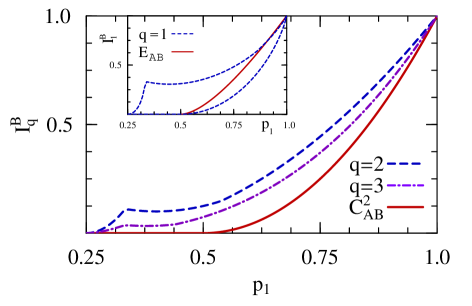
Figure 1: The maximum and minimum values reached by the quantum correlation measures $I_{2}^{B}(\rho_{AB})$ and $I_{3}^{B}(\rho_{AB})$ in the state (38), Eqs. (43)–(45), as a function of its maximum eigenvalue $p_{1}$. The common minimum is just the squared concurrence $C^{2}_{AB}$, whereas the respective maximum is indicated by the dashed and dashed-dotted lines. The inset depicts the maximum and minimum values reached in this state by $I_{f}^{B}$ in the von Neumann case ($q=1$, $log=log_{2}$), where it coincides with the quantum discord, with the solid line depicting the entanglement of formation. The least disturbing measurement is here the same for all entropies, and along the direction of the main principal axis of $J^{t}J$ (see text). Quantities plotted are dimensionless in all figures.

Fig. 1 depicts the maximum and minimum values reached by $I_{2}^{B}$ and $I_{3}^{B}$ in the states (38) for fixed values of the maximum eigenvalue $p_{1}$. The common minimum is just the squared concurrence $C^{2}_{AB}$, reached for $p_{3}=p_{4}=0$ if $p_{1}\geq 1/2$ (and $p_{2}=p_{1}$, $p_{3}=p_{4}$ if $p_{1}\leq 1/2$). The maximum is reached for $p_{2}=p_{3}=p_{4}$ if $p_{1}\geq 7/13\approx 0.54$ for $I_{2}$ and $p_{1}\gtrsim 0.44$ for $I_{3}$, and for $p_{2}=p_{3}$, $p_{4}=0$, if $p_{1}$ lies below the previous values and above $1/3$. As a result, the maximum values for zero concurrence of $I_{2}$ and $I_{3}$ within these states are $1/8$ and $2/27$ respectively, obtained at $p_{1}=1/2$.

In contrast, in the von Neumann case the minimum (again obtained for $p_{3}=p_{4}=0$ if $p_{1}\geq 1/2$) lies clearly below $E_{AB}$ $\forall$ $p\in(1/2,1)$, and even the maximum (attained at $p_{2}=p_{3}=p_{4}$ if $p\gtrsim 0.86$ and $p_{2}=p_{3}$, $p_{4}=0$ if $1/3\leq p_{1}\lesssim 0.86$) lies below $E_{AB}$ if $p_{1}\gtrsim 0.91$. If $p\leq 1/3$ the maximum in these three measures is reached for $p_{2}=p_{3}=p_{1}$.

III.2 States with parity symmetry

Let us now consider the case where both $\bm{r}_{A}$ and $\bm{r}_{B}$ are directed along the same principal axis, i.e., $\bm{r}_{B}$ along $\bm{k}$ and $\bm{r}_{A}$ along $J\bm{k}$, with $\bm{k}$ an eigenvector of $J^{t}J$ (and hence, $J\bm{k}$ an eigenvector of $JJ^{t}$). Choosing these axes as the local $z$ axes, such that $\bm{r}_{A}=r_{A}\bm{k}_{z}$, $\bm{r}_{B}=r_{B}\bm{k}_{z}$ and $J_{\mu\nu}=J_{\mu}\delta_{\mu\nu}$, such state can be written as

$$\rho_{AB} = {\textstyle\frac{1}{4}}(I+r_{A}\sigma_{Az}+r_{B}\sigma_{Bz}+\sum_{\mu=x,y,z}J_{\mu}\sigma_{A\mu}\sigma_{B\mu})$$ (49)

$$= \frac{1}{4}\left(\begin{array}[]{cccc}a_{+}&0&0&\alpha_{+}\\ 0&c_{+}&\alpha_{-}&0\\ 0&\alpha_{-}&c_{-}&0\\ \alpha_{+}&0&0&a_{-}\end{array}\right),\begin{array}[]{rcl}a_{\pm}&=&1+J_{z}\pm(r_{A}+r_{B})\\ c_{\pm}&=&1-J_{z}\pm(r_{A}-r_{B})\\ \alpha_{\pm}&=&J_{x}\mp J_{y}\end{array}.$$ (57)

where the matrix is the representation in the standard basis of $\sigma_{Az}\sigma_{Bz}$ eigenstates. This state commutes with the spin parity RCM.08 $P_{z}=-\exp[i\pi(\sigma_{Az}+\sigma_{Bz})/2]$. It is also denoted as an $X$ state AR.10 .

We will now show that a measurement of $\bm{\sigma}_{B}$ along any of the principal axes $x,y,z$ will provide a stationary point of $I_{f}^{\bm{k}}$ $\forall$ $S_{f}$.
Proof: For a measurement along the $z$ axis ($\bm{k}=\bm{k}_{z}$), i.e., along the axis where $\rho_{B}$ is diagonal, $J^{t}J\bm{k}_{z}=J_{z}^{2}\bm{k}_{z}$, $\bm{r}_{A}$ and $\bm{r}_{B}$ are all along this axis and Eq. (19) is then trivially satisfied $\forall$ $\alpha_{i}$. It is a particular case of Eq. (15), which here holds in the standard basis.

For a measurement along the $x$ axis ($\bm{k}=\bm{k}_{x}$), $J^{t}J\bm{k}_{x}=J_{x}^{2}\bm{k}_{x}$ while $\bm{r}_{B}\cdot\bm{k}_{x}=0$ and $|\bm{r}_{A}+\nu J\bm{k}_{x}|=\sqrt{r_{A}^{2}+J_{x}^{2}}$. Hence ${p}^{\mu}_{\nu}=\frac{1}{4}(1+\mu|\bm{r}_{A}+\nu J\bm{k}_{x}|)$ is independent of $\nu$. This leads to $\alpha_{1}=\alpha_{2}=0$ in (20), in which case Eq. (19) is again satisfied. For $\bm{k}=\bm{k}_{y}$ the argument is similar. We also remark that these arguments also apply to the quantum discord (11), as $\eta=0$ in (23) for $\bm{k}=\bm{k}_{x}$ or $\bm{k}_{y}$.

While other stationary directions may also exist, the principal axes are strong candidates for minimizing $I_{f}^{\bm{k}}$. Typically, the minimum will be attained for measurements along $z$ if ${\rm Max}[|J_{x}|,|J_{y}|]$ is sufficiently small, while otherwise measurements along $x$ or $y$ will be preferred. A transition between these two regimes will arise as $J_{x}$ or $J_{y}$ increases, whose details will depend on the entropic function and may involve intermediate directions $\bm{k}$.

Writing $\bm{k}=(\sin\gamma\cos\phi,\sin\gamma\sin\phi,\cos\gamma)$, these intermediate solutions can be found from Eq. (19), which leads here to $\phi=0$ or $\phi=\pi/2$ (if $|J_{x}|>|J_{y}|$ the minimum corresponds to $\phi=0$ for any $S_{f}$, as the ensuing distribution majorizes that for $\phi=\pi/2$) and to $\gamma=0$ or

$$\cos\gamma=\frac{\alpha_{1}r_{B}+\alpha_{2}J_{z}r_{A}}{\alpha_{3}(J_{x}^{2}-J_{z}^{2})}\,,$$ (58)

where we have assumed $|J_{x}|>|J_{y}|$ such that $\phi=0$. The intermediate solutions $|\gamma|\in(0,\pi/2)$ of (58), if existent, are degenerate, as both choices $\pm\gamma$ lead to the same $I_{f}^{\bm{k}}$. Just the principal axes solutions are non-degenerate.

The final expression for $I_{f}^{B}$ is formally

$$I_{f}^{B}(\rho_{AB})=\sum_{\mu,\nu=\pm}f({p}^{\mu}_{\nu})-f(\lambda^{\mu}_{\nu})\,,$$ (59)

where ${p}^{\mu}_{\nu}=\frac{1}{4}(1+\nu r_{B}k_{z}+\mu\sqrt{(r_{A}+\nu J_{z}k_{z})^{2}+J^{2}_{x}k^{2}_{x}})$ are the eigenvalues (21) of $\rho^{\prime}_{AB}$ and $\lambda^{\mu}_{\nu}$ those of $\rho_{AB}$:

$$\lambda^{\mu}_{\nu}={\textstyle\frac{1}{4}}[1+\nu J_{z}+\mu\sqrt{(r_{A}+\nu r_{B})^{2}+(J_{x}-\nu J_{y})^{2}}]\,.$$ (60)

We can verify the previous results in the quadratic and cubic cases. For an $X$ state both matrices $M_{2}$ and $M_{3}$ (Eqs. (26), (32)) are diagonal in the principal axes basis:

$$M_{2_{\mu\nu}} = \delta_{\mu\nu}(J_{\mu}^{2}+\delta_{\mu z}r_{B}^{2})\,,$$

$$M_{3_{\mu\nu}} = \delta_{\mu\nu}[J_{\mu}^{2}+\delta_{\mu z}(r_{B}^{2}+2r_{B}r_{A}J_{z})]\,.$$

Hence, the optimum measurement will be along the axis with the maximum diagonal value and no intermediate solutions will arise (for non-degenerate eigenvalues), as opposed to the general case. Assuming $|J_{y}|<|J_{x}|$, a “sharp” $z\rightarrow x$ transition for the least disturbing measurement will then take place, the $x$ axis preferred for

$$J_{x}^{2} > J_{z}^{2}+r_{B}^{2}\,,\;\;q=2\,,$$ (61)

$$J_{x}^{2} > J_{z}^{2}+r_{B}^{2}+2r_{B}r_{A}J_{z}\,,\;\;q=3$$ (62)

in the quadratic and qubic cases respectively, such that

$$I_{2}^{B}(\rho_{AB}) = \mbox{$\frac{1}{2}$}\{J_{y}^{2}+{\rm Min}[J_{x}^{2},r_{B}^{2}+J_{z}^{2}]\}\,,$$ (63)

$$I_{3}^{B}(\rho_{AB}) = {\textstyle\frac{1}{4}}\{J_{y}^{2}-2J_{x}J_{y}J_{z}+{\rm Min}[J_{x}^{2},r_{B}^{2}+J_{z}^{2}+2r_{A}r_{B}J_{z}]\}\,.$$

These expressions are in general no longer upper bounds to the squared concurrence, which for these states is $C_{AB}=\frac{1}{2}{\rm Max}[|\alpha_{+}|-\sqrt{c_{+}c_{-}},|\alpha_{-}|-\sqrt{a_{+}a_{-}},0]$. Nonetheless, $I_{2}^{B}$ remains an upper bound to $C_{AB}^{2}$ in the “$z$ phase”, as $C_{AB}^{2}\leq\frac{1}{4}(J_{x}\pm J_{y})^{2}\leq\frac{1}{2}(J_{x}^{2}+J_{y}^{2})$.

III.3 Mixture of aligned states

As a particular relevant example of Eq. (49), we will consider the mixture of two states with spins aligned along different directions. Choosing the $z$ axis as the bisector, such state can be written as

$$\rho_{AB} = \mbox{$\frac{1}{2}$}(|\theta\theta\rangle\langle\theta\theta|+|-\theta-\theta\rangle\langle-\theta-\theta|)$$ (65)

$$= \frac{1}{4}\left(\begin{array}[]{cccc}a_{+}&0&0&c\\ 0&c&c&0\\ 0&c&c&0\\ c&0&0&a_{-}\end{array}\right)\,,\begin{array}[]{rcl}a_{\pm}&=&(1\pm\cos\theta)^{2}\\ c&=&\sin^{2}\theta\end{array}\,,$$ (72)

which corresponds to $(J_{x},J_{y},J_{z})=(\sin^{2}\theta,0,\cos^{2}\theta)$ and $r_{A}=r_{B}=\cos\theta$ in (49). Here

$${\textstyle|\theta\rangle=\exp[-i\frac{\theta}{2}\sigma_{y}]|0\rangle=\cos\frac{\theta}{2}|0\rangle+\sin\frac{\theta}{2}|1\rangle}$$ (73)

is the state with the spin forming an angle $\theta$ with the $z$ axis in the $x,z$ plane. The relevance of this state was discussed in CRC.10 . It represents, roughly, the state of a spin pair in the definite parity ground state of a finite $n$ spin ferromagnetic type $XY$ spin chain in a transverse field for $|B|<B_{c}$, and the exact state of any pair at the immediate vicinity of the factorizing field RCM.08 (neglecting small coherence terms $\propto\cos^{n-2}\theta$).

This state is separable, i.e., it is a convex mixture of product states RF.89 , and the concurrence $C_{AB}$ accordingly vanishes $\forall$ $\theta$. Nonetheless, it has non-zero discord CRC.10 if $\theta\in(0,\pi/2)$. It will then have non-zero values of any $I_{f}^{B}$ in this interval, with $I_{f}^{B}=I_{f}^{A}$ $\forall$ $S_{f}$ due to the symmetry of the state. For $\theta=0$ it is obviously a pure product state, while for $\theta=\pi/2$ it is a classically correlated state, i.e., diagonal in a standard product basis, implying $I_{f}^{B}(\theta)\equiv I_{f}^{B}(\rho_{AB}(\theta))=0$ for $\theta=0$ or $\theta=\pi/2$ $\forall$ $S_{f}$.

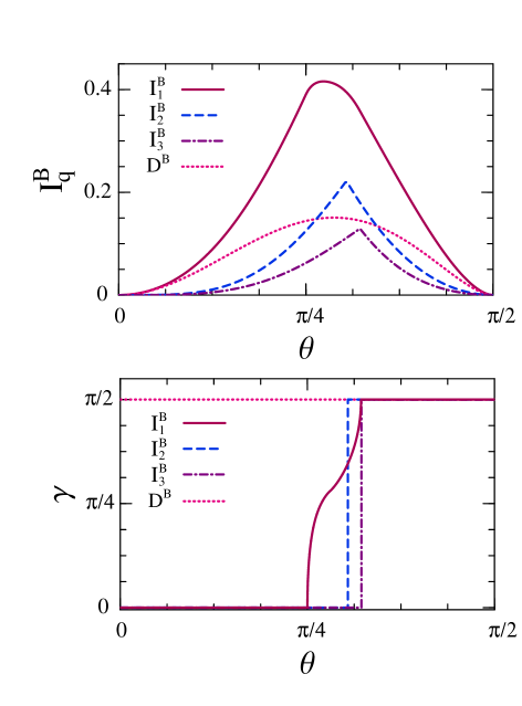
Figure 2: Top: The quantum correlation measures $I_{q}^{B}(\rho_{AB})$ in the state (65), as a function of the angle $\theta$ for $q=1$ (von Neumann case), $2$ and $3$. $D^{B}$ denotes the quantum discord. Bottom: The least disturbing measurement angle $\gamma$ vs. $\theta$ for the same cases depicted above. It is seen that $\gamma$ exhibits a sharp transition from $0$ to $\pi/2$ (i.e., from $z$ to the $x$ axis) in the quadratic $(q=2)$ and cubic $(q=3)$ cases, whereas in the von Neumann case ($q=1$) the transition is smooth. No transition arises in the case of the quantum discord.

It can be expected that as $\theta$ increases, the least disturbing measurement will change from $z$ to $x$. In the quadratic and cubic cases, the transition is sharp. We obtain, according to Eqs. (61)–(LABEL:c5),

$$I_{2} = \mbox{$\frac{1}{2}$}\left\{\begin{array}[]{lr}\sin^{4}\theta&\theta<\theta_{c2}\\ \cos^{2}\theta+\cos^{4}\theta&\theta>\theta_{c2}\end{array},\right.$$ (76)

$$I_{3} = {\textstyle\frac{1}{4}}\left\{\begin{array}[]{lr}\sin^{4}\theta&\theta<\theta_{c3}\\ \cos^{2}\theta+3\cos^{4}\theta&\theta>\theta_{c3}\end{array},\right.$$ (79)

where $\cos^{2}\theta_{c2}=1/3$ ($\theta_{c2}\approx 0.61\pi/2$) and $\cos^{2}\theta_{c3}=(\sqrt{17}-3)/4$ ($\theta_{c3}\approx 0.64\pi/2$), with the minimizing measurement changing from $z$ to $x$ for $\theta>\theta_{ci}$. These two quantities exhibit then a cusp-like maximum at $\theta=\theta_{ci}$, i.e. slightly above $\pi/4$, as seen in Fig. 2.

On the other hand, for other entropies a smooth transition from $z$ to the $x$ direction can arise. For instance, in the von Neumann case $z$ is preferred exactly for $\theta\leq\pi/4$, but $x$ is minimum only for $\theta\gtrsim 0.64\pi/2$. In between, the optimum measurement is obtained for an intermediate angle $\gamma$, as determined by Eq. (58), which varies continuously from $0$ to $\pi/2$, as seen in Fig. 2. This leads to a smooth maximum, located closer to $\pi/4$. In the case of the quantum discord, the minimizing angle is $\gamma=\pi/2$ $\forall$ $\theta$, exhibiting then a different behavior due to the effect of the local term. In this case a relative entropy, rather than a total entropy, is minimized.

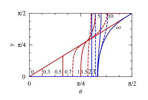
Figure 3: The least disturbing measurement angle $\gamma$ vs. $\theta$ determined by $I_{q}^{B}(\theta)$, for different values of $q$.

For the present state there is no least mixed state $\rho^{\prime}_{AB}$, and the least disturbing measurement depends, therefore, on the entropic function. In order to appreciate previous results from a more general perspective, the behavior of the minimizing angle for different $q$ in the entropies (10) is depicted in Fig. 3. The sharp transition $z\rightarrow x$ (i.e., $0\rightarrow\pi/2$) occurs for $2\leq q\leq 3$, indicating a special critical behavior at these two values. A smoothed transition like that encountered in the von Neumann case arises for $1/2<q<2$ and also $q>3$, where $\gamma$ varies continuously from $0$ to $\pi/2$ within some window of $\theta$ values, which narrows for $q$ close to $2$ or $3$.

For $0<q\leq 1/2$, the minimizing angle changes sharply from $0$ to an intermediate value $\gamma\approx\theta$, increasing then almost linearly with $\theta$ ($\gamma\approx\theta$). This is due to the fact that for low $q$, $S_{q}(\rho^{\prime}_{AB})$ is minimized when the lowest eigenvalue of $\rho^{\prime}_{AB}$ vanishes, and this occurs precisely for $\gamma=\theta$. On the other hand, for high $q$, $S_{q}(\rho^{\prime}_{AB})$ is minimized when the largest eigenvalue of $\rho^{\prime}_{AB}$ is maximum, and the latter is maximized for $\gamma=0$ if $\theta\leq\theta_{c}\approx 0.66\pi/2$, and for an intermediate $\gamma$ if $\theta>\theta_{c}$, which varies continuously from $0$ to $\pi/2$ for $\theta_{c}<\theta<\pi/2$. Accordingly, for high but finite $q$ values, $\gamma=0$ for $\theta\lesssim\theta_{c}$, increasing then with $\theta$ and reaching $\pi/2$ at an increasingly higher $\theta$. Different disorder criteria lead then to different least disturbing measurements in this case, in contrast with the state (38).

IV Conclusions

We have analyzed the determination of the minimum information loss $I_{f}^{B}$ associated with an unread local measurement in a bipartite system, for a general entropy $S_{f}$. Such quantity is a measure of the quantum correlations lost in the local measurement, and reduces to the information deficit and the geometric discord when $S_{f}$ is chosen as the von Neumann and linear entropy respectively. A general stationary condition was derived, together with its explicit form for an arbitrary mixed state of two qubits. Explicit expressions for the cubic entropy and the associated measure $I_{3}^{B}$ were in this case obtained, which require, as in the quadratic case (geometric discord), just the eigenvalues of a $3\times 3$ matrix.

As application, we have first examined two-qubit mixed states with maximally mixed marginals, where the minimum information loss $I_{f}^{B}$ for any entropy was shown to be a simple function of the eigenvalues of $\rho_{AB}$. The minimizing measurement is in this case universal. Moreover, in this case $I_{2}^{B}$ and $I_{3}^{B}$ were shown to be strict upper bounds of the squared concurrence, which is the associated entanglement monotone for both entropies. We have also analyzed the case of $X$ states, providing explicit expressions for $I_{2}^{B}$ and $I_{3}^{B}$ and showing that spin measurements along the principal axes of the matrix $J^{t}J$ are universal stationary points of $I_{f}^{B}$ for any $S_{f}$.

Finally, the special case of a mixture of aligned states was examined in detail. Here the least disturbing local measurement changes, for all measures $S_{f}$, from $z$ (bisector axis) to the $x$ axis as the angle $2\theta$ between both directions changes from $0$ to $\pi$, being then different from that optimizing the original quantum discord (which stays constant), although the type of transition depends on the information measure employed. The least disturbing measurement according to $I_{f}^{B}$ is thus more sensible to the strength of the correlation, and reflects the “transition” experienced by the state. Application of the present formalism to more complex systems is currently under investigation.

The authors acknowledge support of CIC (RR) and CONICET (NC,LC) of Argentina.

References

- (1) C.H. Bennett, D.P. DiVincenzo, J.A. Smolin, and W.K. Wootters, Phys. Rev. A 54, 3824 (1996).
- (2) C.H. Bennett et al., Phys. Rev. Lett. 70, 1895 (1993); Phys. Rev. Lett. 76, 722 (1996).
- (3) M.A. Nielsen and I.L. Chuang, Quantum Computation and Quantum Information (Cambridge Univ. Press, Cambridge, UK, 2000).
- (4) R. Josza and N. Linden, Proc. R. Soc. A 459, 2011 (2003).
- (5) G. Vidal, Phys. Rev. Lett. 91, 147902 (2003).
- (6) E. Knill and R. Laflamme, Phys. Rev. Lett. 81, 5672 (1998).
- (7) A. Datta, S.T. Flammia and C.M. Caves, Phys. Rev. A 72, 042316 (2005).
- (8) R.F. Werner, Phys. Rev. A 40, 4277 (1989).
- (9) H. Ollivier and W.H. Zurek, Phys. Rev. Lett. 88, 017901 (2001).
- (10) L. Henderson and V. Vedral, J. Phys. A 34, 6899 (2001).
- (11) V. Vedral, Phys. Rev. Lett. 90, 050401 (2003).
- (12) W.H. Zurek, Phys. Rev. A 67, 012320 (2003).
- (13) A. Datta, A. Shaji, and C.M. Caves, Phys. Rev. Lett. 100, 050502 (2008).
- (14) M. Horodecki, et al. Phys. Rev. A 71, 062307 (2005); J. Oppenheim, M. Horodecki, P. Horodecki and R. Horodecki, Phys. Rev. Lett. 89, 180402 (2002).
- (15) A. Streltsov, H. Kampermann, and D. Bruß, Phys. Rev. Lett. 106, 160401 (2011).
- (16) B. Dakić, V. Vedral, and Č. Brukner, Phys. Rev. Lett. 105, 190502 (2010).
- (17) R. Rossignoli, N. Canosa, and L. Ciliberti, Phys. Rev. A 82, 052342 (2010).
- (18) K. Modi, et al, Phys. Rev. Lett. 104, 080501 (2010).
- (19) S. Luo, Phys. Rev. A 77, 022301 (2008).
- (20) V. Madhok and A. Datta, Phys. Rev. A 83, 032323 (2011).
- (21) D. Cavalcanti et al, Phys. Rev. A 83, 032324 (2011).
- (22) M. Piani et al, Phys. Rev. Lett. 106, 220403 (2011).
- (23) L. Roa, J.C. Retamal, and M. Alid-Vaccarezza, Phys. Rev. Lett. 107, 080401 (2011).
- (24) A. Shabani and D.A. Lidar, Phys. Rev. Lett. 102, 100402 (2009).
- (25) A. Ferraro et al, Phys. Rev. A 81, 052318 (2010).
- (26) F.F. Fanchini, M. F. Cornelio, M. C. de Oliveira, and A.O. Caldeira, Phys. Rev. A 84, 012313 (2011).
- (27) B.P. Lanyon, M. Barbieri, M.P. Almeida, A.G. White, Phys. Rev. Lett. 101, 200501 (2008).
- (28) A. Datta and S. Gharibian, Phys. Rev. A 79, 042325 (2009).
- (29) S. Luo, Phys. Rev. A 77, 042303 (2008).
- (30) M.S. Sarandy, Phys. Rev. A 80, 022108 (2009).
- (31) T. Werlang, S. Souza, F. F. Fanchini, and C. J. Villas Boas, Phys. Rev. A 80, 024103 (2009).
- (32) M. Ali, A.R.P. Rau, and G. Alber, Phys. Rev. A 81, 042105 (2010); ibid. 82, 069902(E) (2010).
- (33) L. Ciliberti, R. Rossignoli, and N. Canosa, Phys. Rev. A 82, 042316 (2010).
- (34) D. Girolami and G. Adesso, Phys. Rev. A 83, 052108 (2011).
- (35) Y-C. Li and H-Q. Lin, Phys. Rev. A 83, 052323 (2011).
- (36) W.K. Wootters, Phys. Rev. Lett. 80, 2245 (1998).
- (37) P. Rungta and C.M. Caves, Phys. Rev. A 67, 012307 (2003); P. Rungta et al, Phys. Rev. A 64, 042315 (2001).
- (38) R. Rossignoli, N. Canosa and J.M. Matera, Phys. Rev. A 77, 052322 (2008); R. Rossignoli, N. Canosa and J.M. Matera, Phys. Rev. A 80, 062325 (2009).
- (39) N. Canosa and R. Rossignoli, Phys. Rev. Lett. 88, 170401 (2002).
- (40) H. Wehrl, Rev. Mod. Phys. 50, 221 (1978).
- (41) R. Bhatia, Matrix Analysis (Springer-Verlag, New York, 1997).
- (42) R. Rossignoli, N. Canosa, Phys. Rev. A 67, 042302 (2003). R. Rossignoli, N. Canosa, Phys. Rev. A 66, 042306 (2002).
- (43) V. Vedral, Rev. Mod. Phys. 74, 197 (2002).
- (44) C. Tsallis, J. Stat. Phys. 52, 479 (1988); C. Tsallis, Introduction to non-extensive statistical mechanics (Springer, New York, 2009).
- (45) G. Vidal, J. Mod. Opt. 47, 355 (2000).