Non-equilibrium relaxation and critical aging for driven Ising lattice gases

Abstract

We employ Monte Carlo simulations to study the non-equilibrium relaxation of driven Ising lattice gases in two dimensions. Whereas the temporal scaling of the density auto-correlation function in the non-equilibrium steady state does not allow a precise measurement of the critical exponents, these can be accurately determined from the aging scaling of the two-time auto-correlations and the order parameter evolution following a quench to the critical point. We obtain excellent agreement with renormalization group predictions based on the standard Langevin representation of driven Ising lattice gases.

Driven diffusive systems represent paradigmatic models that display non-trivial non-equilibrium stationary states, and hence constitute crucial test cases for various analytical and numerical approaches beatebook ; marrobook . Already driven lattice gases with mere site exclusion and periodic boundary conditions yield anisotropically scale-invariant steady states. In one dimension, the asymptotic scaling properties of these asymmetric exclusion processes are governed by fluctuation-controlled exponents that differ from mean-field predictions; they belong to the noisy Burgers or one-dimensional Kardar–Parisi–Zhang (KPZ) universality class Forster ; kpz . Related models have found varied applications in the theoretical description of biological systems chou2011 . Adding nearest-neighbor attractive Ising interactions, as proposed by Katz, Lebowitz, and Spohn (KLS) katz1983 ; katz1984 to describe ionic conductors, promotes clustering of empty and filled sites, inducing a continuous non-equilibrium phase transition between a disordered and a striped phase in $d\geq 2$ dimensions. In the absence of the drive, one recovers the equilibrium Ising model ferromagnetic phase transition. Yet the correct long-wavelength description of the KLS Ising driven lattice gas at the critical point has been subject to a lasting debate leung1991 ; wang1996 ; schmittmann2000 ; achahbar2001 ; caracciolo2003 ; caracciolo2004_a . Ambiguities in determining the critical exponents are in part caused by exceedingly slow crossovers to the asymptotic regime caracciolo2004_a ; also, it is crucial to implement the proper anisotropic lattice scaling, and infer scaling exponents sufficiently close to the critical point leung1996 .

Intriguing universal scaling features moreover arise in the non-equilibrium relaxation regime from an initial configuration that drastically differs from the final stationary state pleimbook . When the order parameter field is conserved, one may relate the ensuing aging scaling exponents to those describing the non-equilibrium steady state janssen1989 . Investigating the aging and initial-slip scaling regimes thus provides an independent and often more easily accessible means to determine the asymptotic critical exponents zheng1998 . We recently utilized the aging relaxation scaling to accurately confirm the exponent values for asymmetric exclusion processes daquila2011 ; for a related study of the KPZ equation, see Ref. henkel2011 . Critical quenches and the ensuing aging scaling were also analyzed for the continuous phase transition in the contact process baumann2005 ; baumann2007 . Here, we employ Monte Carlo simulations to study the non-equilibrium relaxation properties of the KLS model following a sudden quench from the high-temperature disordered phase to the critical point. We utilize the two-time density auto-correlation function and the temporal evolution of the order parameter in the aging regime of large systems to cleanly measure the associated critical exponents in two dimensions, see also Refs. albano2002 ; albano2011 .

The KLS model consists of $N$ hard-core particles on a $L_{\parallel}\times L_{\perp}^{d-1}$ lattice with periodic boundary conditions; “$\parallel$” and “$\perp$” denote directions parallel and perpendicular to the drive. The occupation number $n_{\bf i}$ at any lattice site ${\bf i}$ is restricted to $0$ or $1$; multiple site occupations are prohibited. In addition to this on-site exclusion, we consider an attractive nearest-neighbor Ising interaction $H_{\rm int}=-J\sum_{\langle{\bf i,j}\rangle}n_{\bf i}\,n_{\bf j}$, $J>0$. The transition rate evolving the system from configuration $X$ to $Y$ then is

$$R(X\to Y)\propto e^{-\beta\left[H_{\rm int}(Y)-H_{\rm int}(X)+\ell E\right]}$$ (1)

with inverse temperature $\beta$; $\ell=\{-1,0,1\}$ indicates particle hops against, transverse to, and along with the drive. The bias $E$ and periodic boundary conditions generate a non-zero particle current through the system; since the rates (1) do not satisfy detailed balance, the system will eventually settle in a non-equilibrium steady state. For $E=0$, and with $n_{\bf i}=\frac{1}{2}(\sigma_{\bf i}+1)$, the KLS lattice gas reduces to the equilibrium Ising model with spin variables $\sigma_{\bf i}=\pm 1$ and conserved Kawasaki kinetics. We employ the standard Metropolis algorithm with rates (1), setting $J=1$ and limiting our study to the case $E\to\infty$, implying that particle jumps with $\ell=-1$ are strictly forbidden. Time is measured in Monte Carlo sweeps, wherein on average one update per particle is attempted.

The theoretical treatment of the long-time and large-scale properties of the KLS model uses a continuum description in terms of a density field $\rho(\vec{x},t)$ or equivalently the conserved spin density $\phi(\vec{x},t)=2\rho(\vec{x},t)-1$. Janssen and Schmittmann janssen1986 as well as Leung and Cardy leung1986 constructed a mesoscopic Langevin equation for the critical KLS model near the critical point,

$$\partial_{t}\phi(\vec{x},t)=\frac{\mathcal{E}}{2}\,\nabla_{\parallel}\phi(\vec{x},t)^{2}-\vec{\nabla}_{\perp}\cdot\vec{\xi}_{\perp}(\vec{x},t)$$ (2)

$$+\lambda\left[\left(c\,\nabla^{2}_{\parallel}+\tau\,\vec{\nabla}^{2}_{\perp}-\vec{\nabla}_{\perp}^{4}\right)\phi(\vec{x},t)+u\,\vec{\nabla}^{2}_{\perp}\phi(\vec{x},t)^{3}\right],$$

and analyzed it by means of perturbative field-theoretic dynamic renormalization group (RG) methods near the upper critical dimension $d_{c}=5$. In the ordered phase, the system forms stripes oriented parallel to the drive, and correspondingly the critical control parameter is $\tau=(T-T_{\rm C})/{T_{\rm C}}\to 0$, whereas $c>0$. $\mathcal{E}$ represents a coarse-grained driving field, with $\mathcal{E}\to{\rm const}$ as $E\to\infty$. Since only the transverse sector becomes critical, just the associated Gaussian noise needs to be accounted for, with $\langle\xi_{\perp}(\vec{x},t)\rangle=0$ and correlator $\langle\xi_{\perp,i}(\vec{x},t)\,\xi_{\perp,j}(\vec{x}^{\prime},t^{\prime})\rangle=n_{\perp}\delta(\vec{x}-\vec{x}^{\prime})\delta(t-t^{\prime})\delta_{ij}$ ($i,j=1,\ldots,d-1$).

We are primarily interested in the density-density correlation function $C(\vec{x},\vec{x}^{\prime},t,s)=\langle\rho(\vec{x},t)\rho(\vec{x}^{\prime},s)\rangle-{\bar{\rho}}^{2}$, with the mean density ${\bar{\rho}}=\langle\rho(\vec{x},t)\rangle=\frac{1}{2}$ in our simulations. Assuming spatial and temporal translational invariance in the non-equilibrium steady state, one arrives at the general scaling form (with positive scale parameter $b$) beatebook

$$C(\vec{x}_{\perp},x_{\parallel},t,\tau,L_{\perp},L_{\parallel})=$$ (3)

$$=b^{d+\Delta-2+\eta}\,C\Bigl{(}\vec{x}_{\perp}b,x_{\parallel}b^{1+\Delta},tb^{z},\tau b^{-1/\nu},L_{\perp}b,L_{\parallel}b^{1+\Delta}\Bigr{)}\,,$$

where $t$, $x_{\parallel}$, and $\vec{x}_{\perp}$ now represent time and position differences. Here, $\nu$ and $z$ denote the transverse correlation length trcorr and dynamic critical exponents, the latter associated with critical slowing-down, while $\eta$ characterizes the power law correlations at criticality. The external drive induces spatially anisotropic scaling, captured by a nonzero anisotropy exponent $\Delta$ (in the mean-field approximation $\Delta=1$), which in turn results in distinct exponents in the direction of the drive, $\nu_{\parallel}=\nu(1+\Delta)$, whence $z_{\parallel}=z/(1+\Delta)$, and $\eta_{\parallel}=(\eta+2\Delta)/(1+\Delta)$ beatebook . In the RG analysis near the upper critical dimension $d_{c}=5$ as determined by the coupling associated with the drive $\mathcal{E}$, the static nonlinearity $u$ becomes (dangerously) irrelevant, and the overall conservation law together with Galilean invariance fix the scaling exponents to all orders in the $\epsilon=5-d$ expansion janssen1986 ; leung1986 . The resulting exact numerical values (henceforth referred to as “JSLC”) are listed in Table 1 for $\epsilon>0$, and specifically for $d=2$.

Table 1: Critical exponents for the KLS and RDLG models (precise definitions are provided in the text).

	JSLC – exact		RDLG – $O(\varepsilon^{2})$
	$\epsilon=5-d$	$d=2$	$\varepsilon=3-d$	$d=2$
$\Delta$	$1+\epsilon/3$	$2$	$1-2\varepsilon^{2}/243$	$0.992$
$z$	$4$	$4$	$4-4\varepsilon^{2}/243$	$3.984$
$\nu$	$1/2$	$1/2$	$\frac{1}{2}+\frac{\varepsilon}{12}+\frac{\varepsilon^{2}}{18}\bigl{[}\frac{67}{108}+\ln\bigl{(}\frac{2}{\sqrt{3}}\bigr{)}\bigr{]}$	$0.626$
$\eta$	$0$	$0$	$4\varepsilon^{2}/243$	$0.016$
$\beta$	$1/2$	$1/2$	$\frac{\nu}{2}\left(1+\Delta-\varepsilon+\eta\right)$	$0.315$
$\zeta$	$1-\epsilon/6$	$1/2$	$\bigl{(}2-\varepsilon+\frac{2\varepsilon^{2}}{243}\bigr{)}/\bigl{(}4-\frac{4\varepsilon^{2}}{243}\bigr{)}$	$0.253$

Early Monte Carlo simulation data valles1987 ; marro1987b ; wang1989 of the critical KLS model with infinite drive indicated discrepancies with these JSLC predictions. Leung leung1991 subsequently applied careful anisotropic finite-size scaling to his Monte Carlo data, and obtained agreement with the JSLC theory, also supported by later work caracciolo2003 ; caracciolo2004_a . A debate on the validity and implications of his results followed achahbar1995 ; leung1996 , and it was proposed garrido1998 ; santos1999 ; garrido2000 that the critical KLS model at infinite drive might not be adequately described by Eq. (2) in the asymptotic limit, but instead by the Langevin equation for the randomly driven Ising lattice gas (RDLG, or two-temperature model B) schmittmann1991 ,

$$\partial_{t}\phi(\vec{x},t)=-\nabla_{\parallel}\xi_{\parallel}(\vec{x},t)-\vec{\nabla}_{\perp}\cdot\vec{\xi}_{\perp}(\vec{x},t)$$ (4)

$$+\lambda\left[\left(c\,\nabla^{2}_{\parallel}+\tau\,\vec{\nabla}^{2}_{\perp}-\vec{\nabla}_{\perp}^{4}\right)\phi(\vec{x},t)+u\,\vec{\nabla}^{2}_{\perp}\phi(\vec{x},t)^{3}\right].$$

Here the drive term $\sim\mathcal{E}$ that is the origin of the non-vanishing particle current has been dropped, with the reasoning that the presence of anisotropic noise with different strengths $n_{\perp}$ and $n_{\parallel}$ is supposedly more relevant in the infinite drive limit. The fluctuations for the Langevin equation (4) are controlled by the static nonlinearity $u$ with upper critical dimension $d_{c}^{\prime}=3$. Dynamic RG methods had earlier been employed to determine the associated critical exponents to two-loop order in a dimensional $\varepsilon=3-d$ expansion schmittmann1991 ; schmittmann1993 ; praestgaard2000 ; the resulting explicit values are also listed in Table 1. However, numerical data for various finite-size scaling functions by Caracciolo et al. favor the JSLC rather than RDLG description caracciolo2005 .

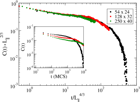
Figure 1: (color online.) Finite-size scaling of the steady-state density auto-correlation function for $(L_{\parallel},L_{\perp})=(54,24)$, $(128,32)$, and $(250,40)$ at the numerically determined “critical temperatures” for these three system sizes according to Eq. (5); the data are averaged over $2000$, $550$, and $200$ realizations, respectively. The inset depicts the unscaled data.

We have performed extensive Metropolis Monte Carlo simulations for the critical KLS model, based on the rates (1) to numerically determine the steady-state scaling exponents. To account for the anisotropic scaling laws, the simulations should be run with properly scaled system extensions, where $L_{\parallel}=\mathcal{A}L_{\perp}^{1+\Lambda}$, where $\Lambda=\Delta$ coincides with the correct anisotropy exponent, such that $\mathcal{A}={\rm const}$. If $\Lambda\neq\Delta$ is chosen, $\mathcal{A}$ does not remain constant and will enter the finite-size scaling functions as an additional relevant variable leung1991 ; caracciolo2005 , see also Ref. caracciolo2003b . Setting $b=L_{\parallel}^{-1/(1+\Delta)}$, $\tau=0$, and letting $\vec{x}_{\perp},x_{\parallel}\to 0$, Eq. (3) reduces to the steady-state finite-size scaling form for the density auto-correlation function at criticality,

$$C(t,L_{\parallel})=L_{\parallel}^{-(d+\Delta-2+\eta)/(1+\Delta)}\,\hat{C}_{\rm FS}\Bigl{(}t/L_{\parallel}^{z_{\parallel}}\Bigr{)}\,.$$ (5)

Following Ref. wang1996 , we determined the finite-size “critical temperatures” $T_{\rm C}^{L_{\parallel}\times L_{\perp}}$ for three different system extensions $(L_{\parallel},L_{\perp})=(54,24)$, $(128,32)$, and $(250,40)$ (i.e., $\mathcal{A}=256$ with $\Lambda=2$) by locating the maximum of the variance of the order parameter fluctuations in the steady state, resulting in $T_{\rm C}^{54\times 24}=0.773$, $T_{\rm C}^{128\times 32}=0.782$ and $T_{\rm C}^{250\times 40}=0.788$ daquila_thesis_2011 . As shown in Fig. 1, we thus achieve reasonable but certainly not unambiguous data collapse using Eq. (5) with the JSLC exponents $z_{\parallel}=\frac{4}{3}$ and $z_{\parallel}\,\zeta=(d+\Delta-2+\eta)/(1+\Delta)=\frac{2}{3}$ at $d=2$ (Table 1). We also performed simulations at the critical temperature in the thermodynamic limit $T_{\rm C}^{\infty}=1.41\,T_{\rm C}^{\rm eq}=0.800$ katz1983 ; valles1987 ; leung1991 ; wang1996 ; achahbar2001 ; albano2002 ; caracciolo2004_a , where $T_{\rm C}^{\rm eq}=0.5673\,J$ is the equilibrium critical point of the square Ising lattice onsager1944 , and found no noticeable quality difference in the scaling collapse. The data in Fig. 1 highlight the difficulty in obtaining accurate critical scaling in the steady state; the density correlations display an extended crossover regime before reaching their asymptotic behavior caracciolo2004_a .

We therefore next venture to determine the critical exponents via a careful aging scaling analysis of the density auto-correlation relaxation to the non-equilibrium steady state. Initiating the simulation runs with a random particle distribution allows us to investigate the out-of-equilibrium relaxation regime wherein time translation invariance is broken, and two-point correlations become explicit functions of two time variables $s$ (referred to as waiting time) and $t>s$ pleimbook . If a system is quenched to the critical point, the initial time sheet may in principle induce novel infrared singularities, as is the case for the relaxational model A with non-conserved order parameter janssen1989 . In contrast, for model B and indeed any system with a diffusive conserved order parameter field, no new divergences emerge, and the critical initial-slip and aging regimes are governed by the steady-state scaling exponents janssen1989 ; zheng1998 ; daquila2011 . We may therefore simply add the waiting time $s$ as independent scaling variable to Eq. (3); setting $b=s^{-1/z}$ then yields the simple aging scaling form of the critical density auto-correlation function,

$$C(t,s)=s^{-\zeta}\,f(t/s)\,,\quad\zeta=(d+\Delta-2+\eta)/z\ .$$ (6)

Our simulation data for the two-time density auto-correlations at $T_{\rm C}^{\infty}$ are displayed in Fig. 2, for anisotropic lattices with $\Lambda=\Delta^{\rm JSLC}$; simulation runs with $\Lambda=\Delta^{\rm RDLG}$ yield virtually identical results daquila_thesis_2011 . The left panel, with the unscaled data plotted vs. $t-s$, confirms that time translation invariance is indeed broken; in the middle and right-hand panel, respectively, we attempt to scale the data either using the JSLC or RDLG exponent values from Table 1. The JSLC exponents manifestly yield excellent data collapse, far superior to the RDLG values.

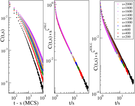
Figure 2: (color online.) Aging scaling plots for the two-time density auto-correlation function following a quench to the critical point from a high-temperature initial state, on a lattice with dimensions $L_{\parallel}=125000$, $L_{\perp}=50$ ($\Lambda=\Delta^{\rm JSLC}=2$). Left panel: unscaled data vs. $t-s$; middle and right panels: scaling plots, Eq. (6), using the JSLC and RDLG exponents, respectively. Each curve is averaged over $200$ realizations.

Moreover, in order to determine the aging exponent in an unbiased manner, we assumed simple aging and obtained $\zeta$ by means of the minimization technique described in Ref. bhattacharjee2001 , resulting in $\zeta\approx 0.48$, in good agreement with the JSLC prediction at $d=2$.

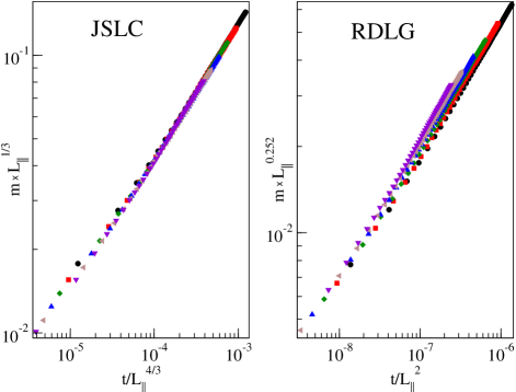
Figure 3: (color online.) Finite-size scaling for the order parameter according to Eq. (9). The data and $L_{\parallel}\times L_{\perp}$ symbols are the same as in Fig. 4, which depicts the asymptotic temporal power law. Left panel: excellent data collapse using the JSLC exponents; right panel: attempted data collapse with RDLG values. Each curve is averaged over $500$ realizations.

Another commonly studied quantity is the anisotropic order parameter, defined in the spin representation as

$$m(t,\tau,L_{\perp},L_{\parallel})=\frac{\sin(\pi/L_{\perp})}{2L_{\parallel}}\,\bigg{|}\displaystyle\sum_{j,k=1}^{L_{\perp},L_{\parallel}}\sigma_{j,k}(t)\,e^{\imath\,2\pi j/L_{\perp}}\bigg{|}\,,$$ (7)

which is sensitive to the density modulations transverse to the drive leung1991 ; wang1996 . Its finite-size scaling over a range of temperatures near the critical point in the steady state is known to be sensitive to the precise location of the critical temperature and the “critical region” chosen for the data analysis leung1996 ; stationary finite-size scaling attempts have consequently resulted in varying values of the order parameter exponent $\beta$ valles1987 ; marro1987b ; wang1989 ; leung1991 ; achahbar1995 ; marro1996 ; wang1996 ; achahbar2001 ; caracciolo2003 ; caracciolo2004_a . We focus on the temporal evolution of the order parameter (7); near $T_{c}$ and beyond mere microscopic time scales, it is governed by the universal scaling law janssen1989 ; caracciolo2004b

$$m(t,\tau,L_{\parallel})=b^{-\beta/\nu_{\parallel}}\,\breve{m}\Bigl{(}\!b^{-z_{\parallel}}t,b^{1/\nu_{\parallel}}\tau,b^{1/(1+\Delta)}L_{\perp}^{-1},bL_{\parallel}^{-1}\!\Bigr{)}.$$ (8)

Identifying $b=L_{\parallel}$ yields the critical finite-size scaling

$$m(t,L_{\parallel})=L_{\parallel}^{-\beta/\nu_{\parallel}}\,\hat{m}\Bigl{(}t/L_{\parallel}^{z_{\parallel}}\Bigr{)}\ .$$ (9)

We present our Monte Carlo simulation results in Fig. 3, employing two-dimensional anisotropic lattices with $\Lambda=\Delta^{\rm JSLC}$. We attempted to scale the data via Eq. (9) using both JSLC and RDLG exponent values, see Table 1; the JSLC critical exponents $z_{\parallel}=\frac{4}{3}$ and $\beta/\nu_{\parallel}=\frac{1}{3}$ clearly give superior data collapse in this “initial slip” region.

To extract the asymptotic temporal power law in the initial slip regime, which allows us to investigate very large systems, we set $b=t^{1/z_{\parallel}}$ and $\tau=0$ in Eq. (8), whence $m(t,L_{\parallel})=t^{-\beta/z_{\parallel}\nu_{\parallel}}\,\widetilde{m}\Bigl{(}t^{1/z}L_{\perp}^{-1},t^{1/z_{\parallel}}L_{\parallel}^{-1}\Bigr{)}$. Substituting $L_{\perp}=\mathcal{A}\,L_{\parallel}^{1/(1+\Delta)}$ with $\mathcal{A}={\rm const}$, $\widetilde{m}$ becomes a function of $x=t^{1/z_{\parallel}}L_{\parallel}^{-1}$ only. Following the procedure outlined in Ref. zheng1998 , we expand the regular scaling function $\widetilde{m}(x)=\widetilde{m}_{0}+\widetilde{m}_{1}x+\ldots$ for $x\ll 1$; here $\tilde{m}_{0}=0$ as alternating occupied/empty initial conditions were chosen. Ignoring higher-order terms, we arrive at

$$m(t,L_{\parallel})\,L_{\parallel}\sim t^{\kappa}\,,\quad\kappa=(1-\beta/\nu_{\parallel})/z_{\parallel}\ .$$ (10)

Figure 4 demonstrates convincing data collapse with this scaling form. Performing a fit to the $64000\times 40$ lattice data yields $\kappa\approx 0.487$, close to the JSLC value $\frac{1}{2}$ gustavo2003 .

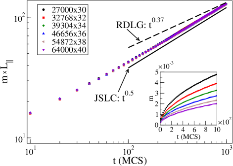
Figure 4: (color online.) Scaling plot according to Eq. (10). The dashed / solid straight lines above / below the simulation data respectively correspond to the predicted RDLG / JSLC power laws. The inset shows the unscaled order parameter growth. Each curve is averaged over $500$ realizations.

In summary, we present detailed Monte Carlo simulation results for the KLS model at criticality confirming the JSLC scaling exponents through the measurement of various dynamical quantities, specifically the order parameter in the initial slip and the two-time density auto-correlation function in the aging regime, which can be numerically accessed for very large lattices. Finite-size scaling of the density auto-correlation function gives satisfactory (if not fully convincing) data collapse with the JSLC exponents. Simple scaling arguments allow us to relate the aging exponent to known steady-state critical exponents janssen1989 ; caracciolo2004b . We have performed Monte Carlo simulations in the transient regime where time translation invariance is broken, and measured the density auto-correlation at different waiting times, thus exploring in detail the universal relaxation features towards a critical non-equilibrium stationary state. The aging exponent inferred from the JSLC exponent values yields convincing data collapse over a range of waiting times, even with different lattice anisotropies. In contrast, the RDLG scaling exponents do not permit a reliable simple aging scaling collapse. The time-dependent order parameter data at short times for different lattice sizes were found to fit a universal master curve using finite-size scaling with JSLC exponents. Applying the same scaling form with RDLG exponents again could not collapse our data. Supporting the conclusions from a careful numerical finite-size scaling analysis caracciolo2005 , our work thus provides strong evidence that the universal features of the critical KLS model are (even with infinite drive) adequately described by the JSLC coarse-grained stochastic Langevin equation, and captured by the associated field-theoretic RG approach.

- (1) B. Schmittmann and R. K. P. Zia, Statistical Mechanics of Driven Diffusive Systems, eds. C. Domb and J. L. Lebowitz (Academic Press, London, 1995).
- (2) J. Marro and R. Dickman, Nonequilibrium Phase Transitions in Lattice Models, (Cambridge University Press, Cambridge, 1999).
- (3) D. Forster, D. R. Nelson, and M. J. Stephen, Phys. Rev. A, 16, 732 (1977).
- (4) M. Kardar, G. Parisi, and Y-C. Zhang, Phys. Rev. Lett. 56, 889 (1986).
- (5) T. Chou, K. Mallick, and R. K. P. Zia, Rep. Prog. Phys. 74, 116601 (2011).
- (6) S. Katz, J. L. Lebowitz, and H. Spohn, Phys. Rev. B 28, 1655 (1983).
- (7) S. Katz, J. L. Lebowitz, and H. Spohn, J. Stat. Phys. 34, 497 (1984).
- (8) K.-t. Leung, Phys. Rev. Lett. 66, 453 (1991).
- (9) J.-S. Wang, J. Stat. Phys. 82, 1409 (1996).
- (10) B. Schmittmann et al., Phys. Rev. E 61, 5977 (2000).
- (11) A. Achahbar, P. L. Garrido, J. Marro, and M. A. Muñoz, Phys. Rev. Lett. 87, 195702 (2001).
- (12) S. Caracciolo, A. Gambassi, M. Gubinelli, and A. Pelissetto, J. Phys. A 36, L315 (2003).
- (13) S. Caracciolo, A. Gambassi, M. Gubinelli, and A. Pelissetto, J. Stat. Phys. 115, 281 (2004).
- (14) K. Leung and R. Zia, J. Stat. Phys. 83, 1219 (1996).
- (15) M. Henkel and M. Pleimling, Ageing and Dynamical Scaling Far from Equilibrium, Nonequilibrium phase transitions Vol. 2 (Springer, Dordrecht, 2010).
- (16) H.K. Janssen, B. Schaub, and B. Schmittmann, Z. Phys. B 73, 539 (1989).
- (17) B. Zheng, Int. J. of Mod. Phys. B 12, 1419 (1998).
- (18) G. L. Daquila and U. C. Täuber, Phys. Rev. E 83, 051107 (2011).
- (19) M. Henkel, J. D. Noh, and M. Pleimling, e-print arXiv: 1109.5022 (2011).
- (20) F. Baumann, M. Henkel, M. Pleimling, and J. Richert, J. Phys. A 38, 6623 (2005).
- (21) F. Baumann and A. Gambassi, J. Stat. Mech. 2007, P01002 (2007).
- (22) E. V. Albano and G. Saracco, Phys. Rev. Lett. 88, 145701 (2002).
- (23) E. V. Albano et al., Rep. Prog. Phys. 74, 026501 (2011).
- (24) H. K. Janssen and B. Schmittmann, Eur. Phys. J. B 64, 503 (1986).
- (25) K. Leung and J. L. Cardy, J. Stat. Phys. 44 (1986).
- (26) Operational definitions for a transverse correlation length in the KLS model are provided in Refs. caracciolo2003 ; caracciolo2004_a .
- (27) J. L. Vallés and J. Marro, J. Stat. Phys. 49, 89 (1987).
- (28) J. Marro, J. L. Vallés, and J. M. González-Miranda, Phys. Rev. B 35, 3372 (1987).
- (29) J.-S. Wang, K. Binder, and J. L. Lebowitz, J. Stat. Phys. 56, 783 (1989).
- (30) A. Achahbar and J. Marro, J. Stat. Phys. 78, 1493 (1995).
- (31) P. L. Garrido, F. de los Santos, and M. A. Muñoz, Phys. Rev. E 57, 752 (1998).
- (32) F. de los Santos and P. L. Garrido, J. Stat. Phys. 96, 303 (1999).
- (33) P. L. Garrido, M. A. Muñoz, and F. de los Santos, Phys. Rev. E 61, R4683 (2000).
- (34) B. Schmittmann and R. K. P. Zia, Phys. Rev. Lett. 66, 357 (1991).
- (35) B. Schmittmann, Europhys. Lett. 24, 109 (1993).
- (36) E. Præstgaard, B. Schmittmann, and R. Zia, Eur. Phys. J. B 18, 675 (2000).
- (37) S. Caracciolo, A. Gambassi, M. Gubinelli, and A. Pelissetto, Phys. Rev. E 72, 056111 (2005).
- (38) S. Caracciolo, A. Gambassi, M. Gubinelli, and A. Pelissetto, Eur. Phys. J. B 34, 205 (2003).
- (39) G. L. Daquila, Ph.D. thesis, Virginia Tech, 2011.
- (40) L. Onsager, Phys. Rev. 65, 117 (1944).
- (41) S. M. Bhattacharjee and F. Seno, J. Phys. A 34, 6375 (2001).
- (42) J. Marro, A. Achahbar, P. L. Garrido, and J. J. Alonso, Phys. Rev. E 53, 6038 (1996).
- (43) S. Caracciolo, A. Gambassi, M. Gubinelli, and A. Pelissetto, Phys. Rev. Lett. 92, 029601 (2004).
- (44) We note that in G. P. Saracco and E. V. Albano, J. Chem. Phys. 118, 4157 (2003), the authors employ a different order parameter definition and scaling ansatz.