Double-layer graphene and topological insulator thin-film plasmons

Abstract

We present numerical and analytical results for the optical and acoustic plasmon collective modes of coupled massless-Dirac two-dimensional electron systems. Our results apply to topological insulator (TI) thin films and to two graphene sheets separated by a thin dielectric barrier layer. We find that because of strong bulk dielectric screening TI acoustic modes are locked to the top of the particle-hole continuum and therefore probably unobservable.

I Introduction

The physics of closely-spaced but unhybridized two-dimensional electron systems (2DESs) has been a subject of theoretical and experimental interest since it was first appreciated pogrebinskii_1977 ; price_physicaB_1983 that electron-electron interactions allow energy and momentum to be transferred between layers, while maintaining separate particle-number conservation. Remote Coulomb coupling has commanded a great deal of attention during the past thirty years or so because it provides a potential alternative to the inductive and capacitive coupling of conventional electronics. Until recently, remote Coulomb coupling research focused on quasi-2D electron systems confined to nearby quantum wells in molecular-beam-epitaxy grown semiconductor heterostructures. The study of Coulomb-coupled 2D systems has now been revitalized by advances which have made it possible to prepare robust and ambipolar 2DESs, based on graphene graphenereviews layers or on the surface states of topological insulators TIreviews , that are described by an ultrarelativistic wave equation instead of the non-relativistic Schrödinger equation.

Single- and few-layer graphene systems can be produced by mechanical exfoliation of thin graphite or by thermal decomposition of silicon carbide SiCreviews . Isolated graphene layers host massless-Dirac two-dimensional electron systems (MD2DESs) with a four-fold (spin $\times$ valley) flavor degeneracy, whereas topologically-protected MD2DESs that have no additional spin or valley flavor labels appear automatically TIreviews ; zhang_natphys_2009 at the top and bottom surfaces of a three-dimensional (3D) TI thin film. The protected surface states of 3D TIs are associated with spin-orbit interaction driven bulk band inversions. 3D TIs in a slab geometry offer two surface states that can be far enough apart to make single-electron tunneling negligible, but close enough for Coulomb interactions between surfaces to be important. Unhybridized MD2DES pairs can be realized in graphene by separating two layers by a dielectric kim_prb_2011 (such as ${\rm Al}_{2}{\rm O}_{3}$) or by a few layers of a one-atom-thick insulator such as BN dean_naturenano_2010 ; ponomarenko_naturephys_2011 . In both cases inter-layer hybridization is negligible and the nearby graphene layers are, from the point of view of single-particle physics, isolated. Isolated graphene layers can be also found on the surface of bulk graphite grapheneongraphite ; li_natphys_2009 and in “folded graphene” schmidt_prb_2010 (a natural byproduct of micromechanical exfoliation), or prepared by chemical vapor deposition li_natphys_2009 . We use the term double-layer graphene (DLG) to refer to a system with two graphene layers that are coupled only by Coulomb interactions, avoiding the term bilayer graphene which typically refers to two adjacent graphene layers in the crystalline Bernal-stacking configuration borghi_prb_2009 .

DLG and TI thin films are both described at low energies by a Hamiltonian with two MD2DES graphenereviews coupled only by Coulomb interactions. The importance of electron-electron interactions in MD2DESs has been becoming more obvious as sample quality has improved eeinteractionsgraphene , motivating investigations of charge and spin or pseudospin dynamics in DLG and thin-film TIs in the regime in which long-range Coulomb forces give rise to robust plasmon collective modes Pines_and_Nozieres ; Giuliani_and_Vignale . Because of their electrically tunable collective behaviors, DLG and thin-film TIs may have a large impact on plasmonics, a very active subfield of optoelectronics Ebbesen_PT_2008 ; Maier07 ; koppens_nanolett_2011 whose aim is to exploit plasmon properties in order to compress infrared electromagnetic waves to the nanometer scale of modern electronic devices.

In this Article we use the random phase approximation (RPA) Pines_and_Nozieres ; Giuliani_and_Vignale to evaluate the optical and acoustic plasmon mode dispersions in DLG and in thin-film TIs. In particular, we obtain an exact analytical formula for the RPA acoustic plasmon group velocity valid for arbitrary substrate and barrier dielectrics that points to a key difference between these two MD2DES’s, namely that the velocity in TI thin films is strongly suppressed. The RPA collective modes of DLG have been calculated earlier by Hwang and Das Sarma hwang_prb_2009 : below we will comment at length on the relation between our results and theirs. Plasmon collective modes formed from TI surface states have also been considered previously by Raghu et al. raghu_prl_2010 in the regime in which coupling between top and bottom surfaces can be neglected. Based on our analysis, we are able to clarify how dielectric screening influences plasma frequencies in this limit.

Plasmons can be observed by a variety of experimental tools including inelastic light scattering pellegrini_review_2006 , which has been widely used to probe plasmons in semiconductor heterostructures plasmonsILSsemiconductors , but also by surface-physics techniques like high-resolution electron-energy-loss spectroscopy liu_prb_2008 , and, more indirectly, angle-resolved photoemission spectroscopy eeinteractionsgraphene . Double-layer field-effect transistors with a grating gate peralta_apl_2002 can also be used to detect plasmons. Coupling between far-infrared light and Dirac plasmons in single-layer graphene has recently been achieved by employing an array of graphene nanoribbons ju_naturenano_2011 and by performing near-field scanning optical microscopy through the tip of an AFM fei_nanolett_2011 .

This manuscript is organized as follows. In Sect. II we present the model we have used to describe a pair of Coulomb-coupled MD2DESs, and introduce the linear-response functions which describe collective electron dynamics. In Sect. III we present and discuss our main analytical and numerical results for the dispersion of optical and acoustic plasmons in these systems. Finally, in Sect. IV we present a summary of our main conclusions.

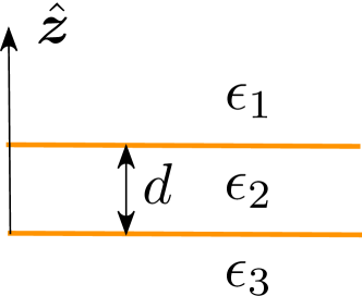
Figure 1: (Color online) A side view of the double-layer system described by Eq. (1), which explicitly indicates the dielectric model used in these calculations. The two layers hosting massless Dirac fermions are located at $z=0$ and $z=d$.

II Model Hamiltonian and Random Phase Approximation

We consider two unhybridized MD2DESs separated by a finite distance $d$ and embedded in the dielectric environment depicted in Fig. 1. The two systems are assumed to be coupled solely by Coulomb interactions. The Hamiltonian describing this system reads profumo_prb_2010 ($\hbar=1$)

$${\hat{\cal H}} = v\sum_{{\bm{k}},\ell,\alpha,\beta}{\hat{\psi}}^{\dagger}_{{\bm{k}},\ell,\alpha}({\bm{\sigma}}_{\alpha\beta}\cdot{\bm{k}}){\hat{\psi}}_{{\bm{k}},\ell,\beta}$$ (1)

$$+ \frac{1}{2S}\sum_{{\bm{q}},\ell,\ell^{\prime}}V_{\ell\ell^{\prime}}(q){\hat{\rho}}_{{\bm{q}},\ell}{\hat{\rho}}_{-{\bm{q}},\ell^{\prime}}~{}.$$

Here $v$ is the bare Dirac velocity, taken to be the same in the $\ell=1,2$ tunnel-decoupled layers, $S$ is the area of each layer, $V_{\ell\ell^{\prime}}(q)$ is the matrix of bare Coulomb potentials, and

$${\hat{\rho}}_{{\bm{q}},\ell}=\sum_{{\bm{k}},\alpha}{\hat{\psi}}^{\dagger}_{{\bm{k}}-{\bm{q}},\ell,\alpha}{\hat{\psi}}_{{\bm{k}},\ell,\alpha}$$ (2)

is the density-operator for the $\ell$-th layer. The Greek letters are honeycomb-sublattice-pseudospin labels and ${\bm{\sigma}}=(\sigma^{x},\sigma^{y})$ is a vector of Pauli matrices. A sum over flavor labels is implicit in Eq. (2) in the case of DLG. The relative strength of Coulomb interactions is measured by the dimensionless coupling constant graphenereviews (restoring $\hbar$ for a moment) $\alpha_{\rm ee}\equiv e^{2}/(\hbar v)$ which has a value $\approx 2.2$ in DLG and $\approx 4.4$ in Bi₂Te₃ TIs if we use the respective Dirac velocities $v_{\rm G}\approx 10^{6}~{}{\rm m}/{\rm s}$ and $v_{\rm TI}\approx 5\times 10^{5}~{}{\rm m}/{\rm s}$.

Several important many-body properties of the Hamiltonian ${\hat{\cal H}}$ are completely determined by the $2\times 2$ symmetric matrix ${\bm{\chi}}(q,\omega)$ whose elements are the density-density linear-response functions

$$\chi_{\ell\ell^{\prime}}(q,\omega)=\frac{1}{S}\langle\langle{\hat{\rho}}_{{\bm{q}},\ell};{\hat{\rho}}_{-{\bm{q}},\ell}\rangle\rangle_{\omega}~{},$$ (3)

with $\langle\langle{\hat{A}},{\hat{B}}\rangle\rangle_{\omega}$ the usual Kubo product. Giuliani_and_Vignale Within the RPA these functions satisfy the following matrix equation,

$${\bm{\chi}}^{-1}(q,\omega)={\bm{\chi}}^{-1}_{0}(q,\omega)-{\bm{V}}(q)~{},$$ (4)

where ${\bm{\chi}}_{0}(q,\omega)$ is a $2\times 2$ diagonal matrix whose elements $\chi^{(0)}_{\ell}(q,\omega)$ are the well-known hwang_prb_2007 ; barlas_prl_2007 ; wunsch_njp_2006 noninteracting (Lindhard) response functions of each layer at arbitrary doping $n_{\ell}$. The off-diagonal (diagonal) elements of the matrix ${\bm{V}}=\{V_{\ell\ell^{\prime}}\}_{\ell,\ell^{\prime}=1,2}$ represent inter-layer (intra-layer) Coulomb interactions.

The bare intra- and inter-layer Coulomb interactions are influenced by the layered dielectric environment (see Fig. 1). A simple electrostatic calculation profumo_prb_2010 implies that the Coulomb interaction in the $\ell=1$ (top) layer is given by

$$V_{11}(q)=\frac{4\pi e^{2}}{qD(q)}[(\epsilon_{2}+\epsilon_{3})e^{qd}+(\epsilon_{2}-\epsilon_{3})e^{-qd}]~{},$$ (5)

where

$$D(q)=[(\epsilon_{1}+\epsilon_{2})(\epsilon_{2}+\epsilon_{3})e^{qd}+(\epsilon_{1}-\epsilon_{2})(\epsilon_{2}-\epsilon_{3})e^{-qd}]~{}.$$ (6)

The Coulomb interaction in the bottom layer, $V_{22}(q)$, can be simply obtained from $V_{11}(q)$ by interchanging $\epsilon_{3}\leftrightarrow\epsilon_{1}$. Finally, the inter-layer Coulomb interaction is given by

$$V_{12}(q)=V_{21}(q)=\frac{8\pi e^{2}}{qD(q)}~{}\epsilon_{2}~{}.$$ (7)

Notice that in the “uniform” $\epsilon_{1}=\epsilon_{2}=\epsilon_{3}\equiv\epsilon$ limit we recover the familiar expressions $V_{11}(q)=V_{22}(q)\to 2\pi e^{2}/(\epsilon q)$ and $V_{12}(q)=V_{21}(q)\to V_{11}(q)\exp(-qd)$. Previous work on TI thin film and DLG collective modes has assumed this limit, which rarely applies experimentally.

III Collective modes

The collective modes of the system described by the model Hamiltonian (1) can be determined by locating the poles of ${\bm{\chi}}(q,\omega)$ in Eq. (4). A straightforward inversion of Eq. (4) yields the following condition dassarma_prb_1981 ; santoro_prb_1988 :

$$\varepsilon(q,\omega) = [1-V_{11}(q)\chi^{(0)}_{1}(q,\omega)][1-V_{22}(q)\chi^{(0)}_{2}(q,\omega)]$$ (8)

$$- V^{2}_{12}(q)\chi^{(0)}_{1}(q,\omega)\chi^{(0)}_{2}(q,\omega)=0~{}.$$

The collective modes occur above the intra-band particle-hole continuum where $\chi^{(0)}$ is real, positive, and a decreasing function of frequency. Eq. (8) admits two solutions, a higher frequency solution hwang_prb_2007 ; wunsch_njp_2006 ; polini_prb_2008 at $\omega_{\rm op}(q)$ which corresponds to in-phase oscillations of the densities in the two layers, and a lower frequency solution at $\omega_{\rm ac}(q)$ which corresponds to out-of-phase oscillations.

The plasmon collective modes of MD2DESs are of special interest because of the ease with which they may be altered by changing the carrier densities in either layer using gates. We note in particular that the carrier densities in different layers can easily differ radically. For this reason we present our results in terms of the total 2D carrier density $n=n_{1}+n_{2}$, and the density polarization $\zeta=(n_{2}-n_{1})/n\in[-1,1]$: $\zeta=1$ when the carrier density is non-zero only in the bottom layer ($n_{1}=0$), while $\zeta=0$ when the two layers have identical carrier densities ($n_{1}=n_{2}$).

III.1 Analytical results

In this Section we report on exact analytical expressions for the RPA optical and acoustic plasmon dispersions $\omega_{{\rm op},{\rm ac}}(q)$ that are valid in the long-wavelength $q\to 0$ limit where $\omega_{\rm op}(q\to 0)\propto\sqrt{q}$ and $\omega_{\rm ac}(q\to 0)\propto q$.

We start by deriving an exact expression for the RPA long-wavelength acoustic-plasmon group velocity,

$$c_{\rm s}=\lim_{q\to 0}\frac{\omega_{\rm ac}(q)}{q}~{}.$$ (9)

Following Santoro and Giuliani santoro_prb_1988 , we first introduce the power expansion

$$\omega_{\rm ac}(q)=c_{\rm s}q+c_{2}q^{2}+c_{3}q^{3}+\dots$$ (10)

for the acoustic-plasmon dispersion relation, and then define a function

$$F(q)=\varepsilon(q,c_{\rm s}q+c_{2}q^{2}+c_{3}q^{3}+\dots)~{}.$$ (11)

In the limit $q\to 0$ the function $F(q)$ has the following Laurent-Taylor expansion

$$F(q)=f_{-1}~{}q^{-1}+f_{0}+f_{1}~{}q+f_{2}~{}q^{2}+\dots~{},$$ (12)

where the coefficients $f_{i}$ can be extracted from the analytical expression barlas_prl_2007 ; hwang_prb_2007 ; wunsch_njp_2006 for the MD2DES Lindhard function $\chi^{(0)}_{\ell}(q,\omega)$. For Eq. (8) to be valid we have to require that the coefficients $f_{i}$ vanish identically. The coefficient $f_{-1}$ depends only on $c_{\rm s}$ and by equating its expression to zero we arrive after some tedious but straightforward algebra at the following equation for $x=c_{\rm s}/v$, the ratio between the plasmon group velocity $c_{\rm s}$ and the Dirac velocity $v$:

$$2g_{\rm s}g_{\rm v}\alpha_{\rm ee}{\bar{d}}(\zeta^{2}-1)[1+2x(\sqrt{x^{2}-1}-x)]$$ (13)

$$- \sqrt{2}\epsilon_{2}[1+x(\sqrt{x^{2}-1}-x)]f(\zeta)=0~{},$$

where $g_{\rm s}$ ($g_{\rm v}$) are real-spin (valley) degeneracy factors. In the case of DLG, $g_{\rm s}=g_{\rm v}=2$, while in the case of thin-film TIs $g_{\rm s}=g_{\rm v}=1$. In Eq. (13) ${\bar{d}}=dk_{\rm F}$ is a dimensionless inter-layer distance calculated with $k_{\rm F}\equiv\sqrt{4\pi n/(g_{\rm s}g_{\rm v})}$ and $n=n_{1}+n_{2}$, and

$$f(\zeta)=(1+\zeta)\sqrt{1-\zeta}+(1-\zeta)\sqrt{1+\zeta}~{}.$$ (14)

Eq. (13) can be conveniently solved for $x$ by making the change of variables $x\mapsto\Gamma=\sqrt{x^{2}-1}-x$. After some straigthforward algebra we find that

$$\frac{c_{\rm s}}{v}=\frac{1+\Lambda(\alpha_{\rm ee}{\bar{d}}/\epsilon_{2},\zeta)}{[1+2\Lambda(\alpha_{\rm ee}{\bar{d}}/\epsilon_{2},\zeta)]^{1/2}}$$ (15)

with

$$\Lambda(\alpha_{\rm ee}{\bar{d}}/\epsilon_{2},\zeta)=\frac{g_{\rm s}g_{\rm v}\sqrt{2}(1-\zeta^{2})}{f(\zeta)}\frac{\alpha_{\rm ee}{\bar{d}}}{\epsilon_{2}}~{}.$$ (16)

Eqs. (15)-(16) are the principle results of this Article. We see from this analytic expression that $c_{\rm s}$ is independent of $\epsilon_{1}$ and $\epsilon_{3}$ and depends only on the barrier material dielectric constant, which in the case of TI thin films is simply the TI bulk dielectric constant. This behavior is a consequence of the out-of-phase character of this collective mode in which the double-layer total charge is locally constant but shifts dynamically between layers. Because TIs tend to have narrow gaps they tend to have large dielectric constants ($\epsilon_{2}\sim 100$ in the caseBiTkappa of Bi₂Te₃). Thin-film collective modes will therefore tend to have $c_{\rm s}/v$ values that are quite close to $1$ unless ${\bar{d}}$ is very large. (For large ${\bar{d}}$ the long-wavelength limit formula, which applies when both $qd$ and $q/k_{\rm F}$ are small, will have a limited range of applicability.)

It follows from Eq. (15) that the ratio $c_{\rm s}/v$ is larger than unity for any value of the parameters $\alpha_{\rm ee}$, ${\bar{d}}$, $\zeta$, and $\epsilon_{2}$ so that the acoustic plasmon always lies outside of the MD2DES particle-hole continuum. This implies than the acoustic plasmon is strictly speaking never Landau damped at small $q$. (A similar conclusion was reached previously santoro_prb_1988 for the case of conventional 2D electron gases, but was limited to the case of identical density and hence identical Fermi velocity.)

For moderate values of $\bar{d}$, however, Eq. (15) predicts a TI thin film sound velocity so close to the top of the particle-hole continuum that it will likely be unobservable because of damping effects not captured by the RPA, and because of disorder, which is always present to some degree. For the case of DLG, on the other hand, we expect that acoustic plasmon collective modes will be well defined. This is particularly true in the case of DLG with a small number of layers of BN as barrier material. When the BN barrier layer is very thin, the use of macroscopic dielectric parameters to characterize its screening properties is approximate; in that case measurement of the acoustic plasmon group velocity combined with Eqs. (15)-(16) would allow the effective value of $\epsilon_{2}$ to be determined experimentally.

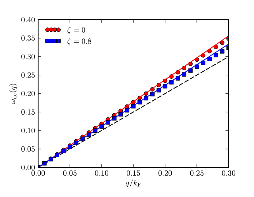
Figure 2: (Color online) Long-wavelength acoustic plasmon dispersion of Coulomb-coupled massless-Dirac two-dimensional electron systems. The circles and squares are acoustic plasmon frequencies $\omega_{\rm ac}(q)$ (in units of $\varepsilon_{\rm F}=vk_{\rm F}$) as functions of $q/k_{\rm F}$ calculated numerically from the solution of Eq. (8). Here $k_{\rm F}$ is the Fermi wave vector evaluated at the total density $n=n_{1}+n_{2}$, i.e. $k_{\rm F}=\sqrt{4\pi(n_{1}+n_{2})/(g_{\rm s}g_{\rm v})}$. The parameters we have used to calculate the curve labeled by “$\zeta=0$” are: $g_{\rm s}=g_{\rm v}=2$, $n_{1}=n_{2}=5\times 10^{12}~{}{\rm cm}^{-2}$, $\alpha_{\rm ee}=2.2$, $d=3.35~{}{\rm\AA}$, $\epsilon_{1}=\epsilon_{2}=1$, and $\epsilon_{3}=3.9$. These parameter values correspond to the case of two graphene layers on ${\rm SiO}_{2}$ that are decoupled by rotation. The data labeled by “$\zeta=0.8$” have been calculated by setting $n_{1}=1\times 10^{12}~{}{\rm cm}^{-2}$ and $n_{2}=9\times 10^{12}~{}{\rm cm}^{-2}$ with the same values for the other parameters. The solid lines plot $\omega=c_{\rm s}q$ for the $\zeta=0$ and $\zeta=0.8$ cases with the plasmon group velocity $c_{\rm s}$ calculated from the analytical result, Eq. (15). These numerical results confirm the validity of our analytic result for $c_{\rm s}$ and the importance of accounting for the delicate dependence of the long-wavelength Lindhard function on $\nu=\omega/(vq)$. The dashed line plots the upper-bound of the intra-band electron-hole continuum, $\omega=vq$.

We note that an analytic result for $c_{\rm s}$ was reported previously in Ref. hwang_prb_2009, [see their Eq. (5b)] for the special case of DLG embedded in a uniform dielectric, i.e. for $\epsilon_{1}=\epsilon_{2}=\epsilon_{3}$. In our notation, their result reads

$$\left.\frac{c_{\rm s}}{v}\right|_{\rm HDS}=\left[\frac{2\sqrt{2}\sqrt{1-\zeta^{2}}}{\sqrt{1-\zeta}+\sqrt{1+\zeta}}\frac{\alpha_{\rm ee}{\bar{d}}}{\epsilon_{2}}\right]^{1/2}~{}.$$ (17)

This equation is evidently different from Eq. (15) above. We believe that Eq. (15) is the correct RPA result for the acoustic-plasmon group velocity and that Eq. (17) is incorrect. The difference is due to the singular behavior of the Lindhard function $\chi^{(0)}_{\ell}(q,\omega)$ as a function of wave vector $q$ and frequency $\omega$ in the region in which both these quantities are small. (See Sect. 4.4.3 of Ref. Giuliani_and_Vignale, .) In particular, the limit of $\chi^{(0)}_{\ell}(q,\omega)$ for $q\to 0$ and $\omega\to 0$ depends on the ratio $\nu=\omega/(vq)$, i.e. on the direction along which the origin of the $(q,\omega)$ plane is approached: different limits are obtained for different values of $\nu$. In an acoustic plasmon, the ratio $\nu$ approaches a constant as $q\to 0$ and thus the limit of $\chi^{(0)}_{\ell}(q,\omega)$ which matters is the one in which $q\to 0$ while the ratio $\omega/q$ is kept constant. This is the limit we have taken santoro_prb_1988 in the derivation of Eq. (15) – see Eq. (11). Eq. (17) is obtained by incorrectly letting $q\to 0$ while $\omega$ is kept constant [see Eq. (4) in Ref. hwang_prb_2009, ]: in this limit $\nu$ diverges instead of going to a constant value.

A careful comparison between our analytical prediction in Eq. (15) and the result obtained by the brute-force numerical solution of Eq. (8) is shown in Fig. 2. We clearly see that Eq. (15) compares very well with the full numerical result.

The analytical analysis of the long-wavelength optical plasmon mode is simpler since this mode satisfies $\omega_{\rm op}(q)\propto\sqrt{q}$ for $q\to 0$ and therefore occurs at $\nu=\omega/(vq)\to\infty$. We obtain an analytic result using the well-known high-frequency ($\omega\gg vq$ and $\omega\ll 2\varepsilon_{{\rm F},\ell}$) dynamical limit of $\chi^{(0)}_{\ell}(q,\omega)$:

$$\lim_{q\to 0}\chi^{(0)}_{\ell}(q,\omega)=g_{\rm s}g_{\rm v}\frac{\varepsilon_{{\rm F},\ell}}{4\pi}\frac{q^{2}}{\omega^{2}}~{},$$ (18)

with $\varepsilon_{{\rm F},\ell}=vk_{{\rm F},\ell}=v\sqrt{4\pi n_{\ell}/(g_{\rm s}g_{\rm v})}$. Using Eq. (18) in Eq. (8) we immediately find

$$\omega^{2}_{\rm op}(q\to 0)=\frac{g_{\rm s}g_{\rm v}\alpha_{\rm ee}}{2\bar{\epsilon}}v^{2}k_{\rm F}\left(\sqrt{\frac{1+\zeta}{2}}+\sqrt{\frac{1-\zeta}{2}}\right)q~{},$$ (19)

with $\bar{\epsilon}=(\epsilon_{1}+\epsilon_{3})/2$. Note that Eq. (19) does not depend on the inter-layer distance or on the dielectric constant $\epsilon_{2}$, but only on the average $\bar{\epsilon}$ between top and bottom dielectric constants. Notice also that, in the limit $n_{1}\to 0$ ($\zeta=1$), Eq. (19) reduces to the well-known plasmon frequency in a single-layer graphene sheet polini_prb_2008 ; hwang_prb_2007 ; wunsch_njp_2006 with electron density $n_{2}$. This expression applies for $qd\ll 1$, in which case the entire double-layer MD2DES acts in the optical plasmon mode like a single conducting layer at the interface between dielectric media characterized by constants $\epsilon_{1}$ and $\epsilon_{3}$.

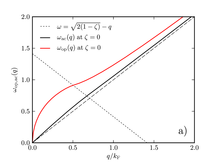
Figure 3: (Color online) Panel a) Optical and acoustic plasmon dispersions (in units of the Fermi energy $\varepsilon_{\rm F}=vk_{\rm F}$) in a twisted double-layer graphene system on a ${\rm SiO}_{2}$ substrate as functions of wave vector $q$ [in units of $k_{\rm F}=\sqrt{4\pi(n_{1}+n_{2})/(g_{\rm s}g_{\rm v})}$]. The values of the parameters that we have used to produce the data in this figure are: $g_{\rm s}=g_{\rm v}=2$, $n_{1}=n_{2}=5\times 10^{12}~{}{\rm cm}^{-2}$ (corresponding to $n=10^{13}~{}{\rm cm}^{-2}$ and $\zeta=0$), $\alpha_{\rm ee}=2.2$, $d=3.35~{}{\rm\AA}$, $\epsilon_{1}=\epsilon_{2}=1$, and $\epsilon_{3}=3.9$. The intersections between the plasmon dispersions and the short-dashed line give the critical wave vector $q_{\rm c}$ at which Landau damping starts. Panel b) Same as in panel a) but for $\zeta=0.5$ [in producing the data shown in panel b) we have fixed the total density at the value used to produce the data in panel a), i.e. $n=10^{13}~{}{\rm cm}^{-2}$].

III.2 Numerical results

In this Section we briefly report some representative numerical results for the optical and acoustic plasmon dispersion relations obtained by solving Eq. (8), discussing first DLG and then TI thin films.

In Fig. 3 we illustrate the typical properties of DLG plasmon modes for the case with the smallest MD2DES separation, two adjacent layers on a ${\rm SiO}_{2}$ substrate ($\epsilon_{1}=\epsilon_{2}=1$ and $\epsilon_{3}=3.9$) that are weakly hybridized e.g. because of a twist between their orientations twistedgraphene . Fig. 3a) is for a symmetric system with the same electron concentration on the two layers ($\zeta=0$), while Fig. 3b) refers to a system with a $50\%$ density imbalance. The characteristic behaviors $\omega_{\rm op}(q)\propto\sqrt{q}$ of the optical plasmon and $\omega_{\rm ac}(q)\propto q$ of the acoustic plasmon are clearly visible. The collective modes are not Landau damped when they appear in the gap between intra-band and inter-band particle-hole continua. When the two layers have different densities, their particle-hole continua are different and the gap is smaller for the lower density layer. For adjacent but twisted DLG systems ${\bar{d}}$ is small even when the carrier density is large ($\bar{d}\approx 0.2$ in Fig. 3). It follows that $qd$ is small and the two MD2DESs are strongly coupled over the entire relevant frequency regime. In this small ${\bar{d}}$ example the acoustic plasmon frequency is close to the particle-hole continuum because the capacitive energy associated with charge sloshing between the layers is proportional to the small layer separation.

In Fig. 4 we illustrate the strength of plasmon decay by emission of single electron-hole pairs (Landau damping). Notice that Landau damping occurs when the curves $\omega_{{\rm op},{\rm ac}}(q)$ in Fig. 3 hit the inter-band electron-hole continuum of the layer with lower density (layer “1” in our convention). The larger $\zeta$, the sooner this happens. In particular, in the limit in which layer “1” is neutral ($\zeta=1$), Landau damping is present from vanishingly small wave vectors: damping of the optical plasmon excitation associated with electrons in the high-density layer starts at arbitrarily small wave vectors since decay can easily occur via the emission of inter-band electron-hole pairs in the neutral layer. The many-body properties of two or more decoupled graphene layers can thus be strongly affected by inter-layer Coulomb interactions, even by apparently innocuous geometric features such as the presence of a nearly-neutral layer.

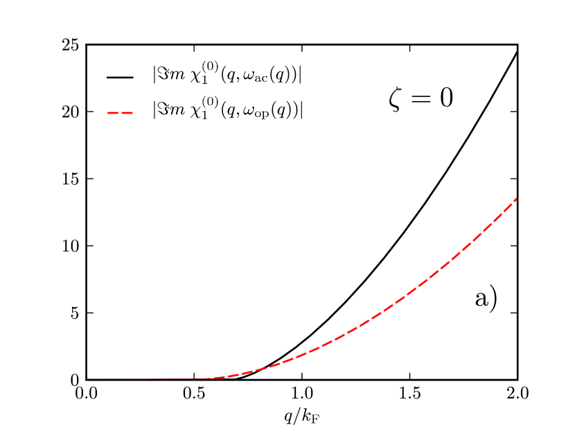
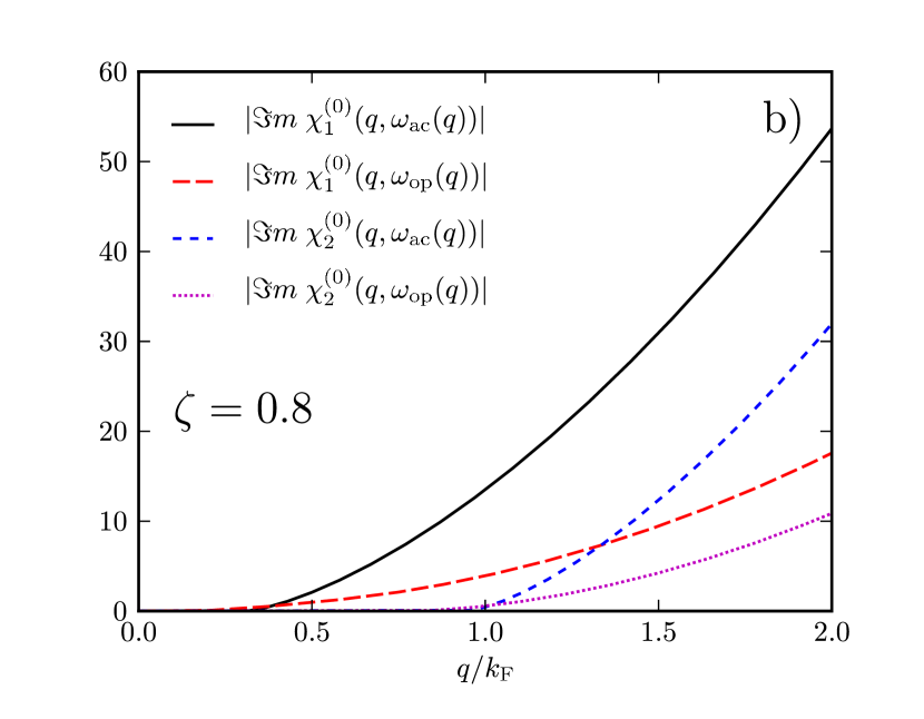
Figure 4: (Color online) Landau damping of collective modes in double-layer graphene. Panel a) The absolute value of the imaginary part of the Lindhard function of the top layer, $|\Im m~{}\chi^{(0)}_{1}(q,\omega)|$, evaluated at the frequency $\omega=\omega_{\rm op}(q)$ [$\omega=\omega_{\rm ac}(q)$] of the optical [acoustic] plasmon. The data in this plot refer exactly to the parameters used in Fig. 3a). Note that, within RPA, $\Im m~{}\chi^{(0)}_{1}(q,\omega_{{\rm op},{\rm ac}}(q))$ is identically zero for wave vectors $q$ up to a critical value $q^{\star}_{{\rm op},{\rm ac}}$ at which $\omega_{{\rm op},{\rm ac}}(q)$ hits the inter-band electron-hole continuum associated with the low-density layer. Since data in this panel correspond to $\zeta=0$, top-layer and bottom-layer Lindhard functions are identical. Panel b) Same as in panel a) but for $\zeta=0.8$ ($n_{1}=1\times 10^{12}~{}{\rm cm}^{-2}$ and $n_{2}=9\times 10^{12}~{}{\rm cm}^{-2}$). Note that the $q^{\star}_{{\rm op},{\rm ac}}$ decreases with increasing $\zeta$ becoming zero in the limit $\zeta\to 1$. Since in this panel $\zeta\neq 0$ we have plotted both top-layer (low-density) and bottom-layer (high-density) Lindhard functions.

In Fig. 5 we compare optical and acoustic plasmon dispersions for DLG and TI thin-film systems. For the TI thin-film case we have chosen the following parameters: i) $\epsilon_{1}=1$, $\epsilon_{2}=100$ (this roughly corresponds to the dielectric constant of ${\rm Bi}_{2}{\rm Te}_{3}$), and $\epsilon_{3}=4.0$; ii) a total electron density on the top and bottom surface states of $n=10^{13}~{}{\rm cm}^{-2}$; and iii) a thickness of the TI slab of $d=6~{}{\rm nm}$, corresponding to a six quintile layer MBE-grown ${\rm Bi}_{2}{\rm Te}_{3}$ film (${\bar{d}}\approx 6.7$). The DLG example has the same total density and layer separation (${\bar{d}}\approx 3.4$; the difference in ${\bar{d}}$ in the two cases stems from the $g_{\rm s}$/$g_{\rm v}$ spin/valley degeneracy factors) and dielectric constants $\epsilon_{1}=1$ and $\epsilon_{2}=\epsilon_{3}=4.0$, corresponding to two graphene layers separated by approximately 15 BN layers and lying on a BN substrate. In both cases we see that a crossover occurs at intermediate values of $q$ between strong (small $q$) and weak (large $q$) coupling of the two collective modes. In the TI case the higher frequency optical plasmon mode deviates much more strongly from simple $\sqrt{q}$ behavior at this crossover because strong dielectric screening by the TI bulk suppresses the single-surface plasmon mode. [Note however that the effective dielectric constant for this limit is $(\epsilon_{2}+\epsilon_{1,3})/2$ rather than $\epsilon_{2}$ as used in Ref. raghu_prl_2010, .] The acoustic plasmon mode of the TI thin film case is, on the other hand, strongly suppressed in the strong-coupling limit, as discusses earlier, and has a velocity much closer to the bare Dirac velocity than in the corresponding DLG case.

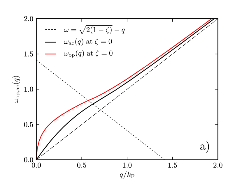
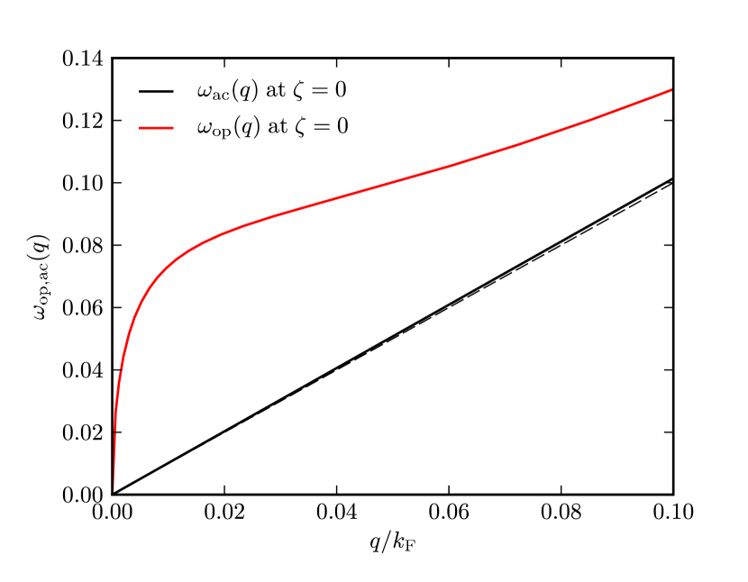
Figure 5: (Color online) Optical and acoustic plasmon dispersions (in units of the Fermi energy $\varepsilon_{\rm F}=vk_{\rm F}$) in a double-layer graphene system [panel a)] and a topological insulator thin-film [panel b)] as functions of wave vector $q$ [in units of $k_{\rm F}=\sqrt{4\pi(n_{1}+n_{2})/(g_{\rm s}g_{\rm v})}$]. The intersections between the plasmon dispersions and the short-dashed line give the critical wave vector $q_{\rm c}$ at which Landau damping starts. Panel a) The values of the parameters that we have used to produce the data in this figure are: $g_{\rm s}=g_{\rm v}=2$, $n_{1}=n_{2}=5\times 10^{12}~{}{\rm cm}^{-2}$ (corresponding to $n=10^{13}~{}{\rm cm}^{-2}$ and $\zeta=0$), $\alpha_{\rm ee}=2.2$, $d=6~{}{\rm nm}$, $\epsilon_{1}=1$, and $\epsilon_{2}=\epsilon_{3}=4.0$. Panel b) The values of the parameters that we have used to produce the data in this figure are: $g_{\rm s}=g_{\rm v}=1$, $n_{1}=n_{2}=5\times 10^{12}~{}{\rm cm}^{-2}$, $\alpha_{\rm ee}=4.4$, $d=6~{}{\rm nm}$, $\epsilon_{1}=1$, $\epsilon_{2}=100$, and $\epsilon_{3}=4.0$. Note that due to the large value of the bulk TI dielectric constant, the acoustic plasmon is almost locked to the top of the intra-band electron-hole continuum.

IV Discussion and conclusions

We have presented an analysis of the electronic collective modes of systems composed of two unhybridized but Coulomb-coupled massless-Dirac two-dimensional electron systems (MD2DESs) separated by a vertical distance $d$. The primary example we have in mind is topological insulator (TI) thin films, which are always described at low energies by this type of model because topologically protected MD2DESs always appear on both top and bottom surfaces. Also of interest are closely related systems, which we refer to as double-layer graphene (DLG) systems, containing two graphene layers that are weakly hybridized either because they are rotated relative to each other or because they are separated by a dielectric barrier layer. Importantly, we allow for a general dielectric environment in which the material above the top MD2DES layer ($\epsilon_{1}$), between the two layers ($\epsilon_{2}$), and below the bottom MD2DES layer ($\epsilon_{3}$) are all allowed to have different dielectric constants. In the case of TI thin film $\epsilon_{2}$ is the bulk dielectric constant of the TI which is expected to have large values. The carrier collective modes of MD2DESs are expected to be most robust in the gap between intraband and interband particle-hole excitations.

The double-layer systems of interest quite generally have two collective modes which in the limit of small $qd$ involve density-fluctuations in the two-layers that are strongly coupled, and in the limit of large $qd$ weakly coupled single-layer plasmons. One key parameter which controls collective mode properties is the dimensionless product $k_{\rm F}d\equiv\bar{d}$. Small values of $k_{\rm F}d$ imply that the layer separation is smaller than the typical distance between electrons within a layer and that collective modes at all values of $q$ up to $\sim k_{\rm F}$ are strongly coupled combinations of the two individual layer density-fluctuation contributions. For large $k_{\rm F}d$ a crossover occurs for $q\in(0,k_{\rm F})$ between strongly and weakly coupled double-layer collective modes. Both small and large values of $\bar{d}$ are achievable in samples where disorder plays an inessential role in both DLG and TI thin film cases.

Our study focuses on the long-wavelength limit in which both $qd$ and $q/k_{\rm F}=qd/\bar{d}$ are small. We have derived analytic expressions for both frequencies of both the low-energy linearly dispersing acoustic plasmon mode $\omega_{\rm ac}(q)$ and for the high-energy optical plasmon mode $\omega_{\rm op}(q)$ which has $\sqrt{q}$ dispersion at long-wavelengths. In this limit we find that $\omega_{\rm ac}(q)-vq\propto 1/\epsilon_{2}$ whereas $\omega_{\rm op}(q)\propto\sqrt{2/(\epsilon_{1}+\epsilon_{3})}$; i.e. the separation of the acoustic plasmon mode from the upper edge of the intra-band particle-hole continuum is very strongly suppressed by a large bulk TI dielectric constant, whereas the coupled double-layer plasmon mode is unaffected. This double-layer optical plasmon behavior contrasts with that of a large $qd$ single-surface plasmon mode which has a frequency proportional to $\sqrt{2/(\epsilon_{2}+\epsilon_{1,3})}$. The long-wavelength limit of $\omega_{\rm ac}(q)$ is sensitive not only to the energy associated with inter-layer charge sloshing but also to its microscopic kinetics as captured by the singular sensitivity of the MD2DES Lindhard function to $\omega/(vq)$. By carefully accounting for this dependence we are able to correct a previous analytic expression in a way that is quantitatively particularly important in the TI thin film (large $\epsilon_{2}$) case.

Double-layer collective mode coupling plays an important role in MD2DES correlations when $\bar{d}$ is small. Even when $\bar{d}$ is large, strongly-coupled small $qd=q\bar{d}/k_{\rm F}$ modes will often be experimentally accessible and may play an important role in graphene multi-layer or TI based plasmonics. The analytic results derived in this paper can be used to readily anticipate how these modes depend on system parameters.

From the more theoretical point of view, it will be intriguing to study physical properties of plasmons in Coulomb-coupled MD2DESs beyond the random phase approximation by employing e.g. many-body diagrammatic perturbation theory abedinpour_prb_2011 .

- (1) M.B. Pogrebinskii, Sov. Phys. Semicond. 11, 372 (1977).
- (2) P.J. Price, Physica 117B, 750 (1983).
- (3) A.K. Geim, Science 324, 1530 (2009); A.H. Castro Neto, F. Guinea, N.M.R. Peres, K.S. Novoselov, and A.K. Geim, Rev. Mod. Phys. 81, 109 (2009); A.K. Geim and K.S. Novoselov, Nature Mater. 6, 183 (2007).
- (4) J. Moore, Nature Phys. 5, 378 (2009); J.E. Moore, Nature 464, 194 (2010); M.Z. Hasan and C.L. Kane, Rev. Mod. Phys. 82, 3045 (2010); X.-L. Qi and S.-C. Zhang, ibid. 83, 1057 (2011).
- (5) E. Rollings, G.-H. Gweon, S.Y. Zhou, B.S. Mun, J.L. McChesney, B.S. Hussain, A.V. Fedorov, P.N. First, W.A. de Heer, and A. Lanzara, J. Phys. Chem. Solids 67, 2172 (2006); W.A. de Heer, C. Berger, X. Wu, P.N. First, E.H. Conrad, X. Li, T. Li, M. Sprinkle, J. Hass, M.L. Sadowski, M. Potemski, and G. Martinez, Solid State Commun. 143, 92 (2007); P.N. First, W.A. de Heer, T. Seyller, C. Berger, J.A. Stroscio, and J.-S. Moon, MRS Bullettin 35(4), 296 (2010).
- (6) See, for example, H. Zhang, C.-X. Liu, X.-L. Qi, Xi Dai, Z. Fang, and S.-C. Zhang, Nature Phys. 5, 438 (2009).
- (7) S. Kim, I. Jo, J. Nah, Z. Yao, S.K. Banerjee, and E. Tutuc, Phys. Rev. B 83, 161401 (2011).
- (8) C.R. Dean, A.F. Young, I. Meric, C. Lee, L. Wang, S. Sorgenfrei, K. Watanabe, T. Taniguchi, P. Kim, K.L. Shepard, and J. Hone, Nature Nanotech. 5, 722 (2010).
- (9) L.A. Ponomarenko, A.K. Geim, A.A. Zhukov, R. Jalil, S.V. Morozov, K.S. Novoselov, I.V. Grigorieva, E.H. Hill, V.V. Cheianov, V.I. Fal’ko, K. Watanabe, T. Taniguchi, and R.V. Gorbachev, Nature Phys. 7, 958 (2011).
- (10) G. Li, A. Luican, and E.Y. Andrei, Phys. Rev. Lett. 102, 176804 (2009); P. Neugebauer, M. Orlita, C. Faugeras, A.-L. Barra, and M. Potemski, ibid. 103, 136403 (2009).
- (11) G. Li, A. Luican, J.M.B. Lopes dos Santos, A.H. Castro Neto, A. Reina, J. Kong, and E.Y. Andrei, Nature Phys. 6, 109 (2009).
- (12) H. Schmidt, T. Lüdtke, P. Barthold, E. McCann, V.I. Fal’ko, and R.J. Haug, Appl. Phys. Lett. 93, 172108 (2008); H. Schmidt, T. Lüdtke, P. Barthold, and R.J. Haug, Phys. Rev. B81, 121403(R) (2010).
- (13) The collective modes of bilayer graphene have already been calculated: see e.g. G. Borghi, M. Polini, R. Asgari, and A.H. MacDonald, Phys. Rev. B80, 241402(R) (2009).
- (14) See, for example, A. Bostwick, T. Ohta, T. Seyller, K. Horn, and E. Rotenberg, Nature Phys. 3, 36 (2007); Z.Q. Li, E.A. Henriksen, Z. Jiang, Z. Hao, M.C. Martin, P. Kim, H.L. Stormer, and D.N. Basov, ibid. 4, 532 (2008); X. Du, I. Skachko, F. Duerr, A. Luican, and E.Y. Andrei, Nature 462, 192 (2009); K.I. Bolotin, F. Ghahari, M.D. Shulman, H.L. Stormer, and P. Kim, ibid. 462, 196 (2009); V.W. Brar, S. Wickenburg, M. Panlasigui, C.-H. Park, T.O. Wehling, Y. Zhang, R. Decker, C. Girit, A.V. Balatsky, S.G. Louie, A. Zettl, and M.F. Crommie, Phys. Rev. Lett. 104, 036805 (2010); E.A. Henriksen, P. Cadden-Zimansky, Z. Jiang, Z.Q. Li, L.-C. Tung, M.E. Schwartz, M. Takita, Y.-J. Wang, P. Kim, and H.L. Stormer, ibid. 104, 067404 (2010); A. Bostwick, F. Speck, T. Seyller, K. Horn, M. Polini, R. Asgari, A.H. MacDonald, and E. Rotenberg, Science 328, 999 (2010); A. Luican, G. Li, and E.Y. Andrei, Phys. Rev. B83, 041405(R) (2011); K.F. Mak, J. Shan, and T.F. Heinz, Phys. Rev. Lett. 106, 046401 (2011); F. Ghahari, Y. Zhao, P. Cadden-Zimansky, K. Bolotin, and P. Kim, ibid. 106, 046801 (2011); D.C. Elias, R.V. Gorbachev, A.S. Mayorov, S.V. Morozov, A.A. Zhukov, P. Blake, L.A. Ponomarenko, I.V. Grigorieva, K.S. Novoselov, F. Guinea, and A.K. Geim, Nature Phys. 7, 701 (2011); D.A. Siegel, C.-H. Park, C. Hwang, J. Deslippe, A.V. Fedorov, S.G. Louie, and A. Lanzara, Proc. Natl. Acad. Sci. USA 108, 11365 (2011).
- (15) D. Pines and P. Noziéres, The Theory of Quantum Liquids (W.A. Benjamin, Inc., New York, 1966).
- (16) G.F. Giuliani and G. Vignale, Quantum Theory of the Electron Liquid (Cambridge University Press, Cambridge, 2005).
- (17) S.A. Maier, Plasmonics – Fundamentals and Applications (Springer, New York, 2007).
- (18) T.W. Ebbesen, C. Genet, and S.I. Bozhevolnyi, Phys. Today 61(5), 44 (2008).
- (19) F.H.L. Koppens, D.E. Chang, and F.J. García de Abajo, Nano Lett. 11, 3370 (2011).
- (20) E.H. Hwang and S. Das Sarma, Phys. Rev. B80, 205405 (2009).
- (21) S. Raghu, S.B. Chung, X.L. Qi and S.-C. Zhang, Phys. Rev. Lett. 104, 116401 (2010).
- (22) For a recent review see e.g. V. Pellegrini and A. Pinczuk, Phys. Stat. Sol. (B) 243, 3617 (2006).
- (23) D.S. Kainth, D. Richards, H.P. Hughes, M.Y. Simmons, and D.A. Ritchie, Phys. Rev. B57, 2065(R) (1998); D.S. Kainth, D. Richards, A.S. Bhatti, H.P. Hughes, M.Y. Simmons, E.H. Linfield, and D.A. Ritchie, ibid. 59, 2095 (1999); D.S Kainth, D. Richards, H.P. Hughes, M.Y. Simmons, and D.A Ritchie, J. Phys.: Condens. Matter 12, 439 (2000); C.F. Hirjibehedin, A. Pinczuk, B.S. Dennis, L.N. Pfeiffer, and K.W. West, Phys. Rev. B65, 161309 (2002); S.V. Tovstonog, L.V. Kulik, I.V. Kukushkin, A.V. Chaplik, J.H. Smet, K.V. Klitzing, D. Schuh, and G. Abstreiter, ibid. 66, 241308 (2002).
- (24) Y. Liu, R.F. Willis, K.V. Emtsev, and T. Seyller, Phys. Rev. B78, 201403(R) (2008); Y. Liu and R.F. Willis, ibid. 81, 081406(R) (2010); R.J. Koch, T. Seyller, and J.A. Schaefer, ibid. 82, 201413(R) (2010). T. Langer, J. Baringhaus, H. Pfnür, H.W. Schumacher, and C. Tegenkamp, New J. Phys. 12, 033017 (2010); C. Tegenkamp, H. Pfnür, T. Langer, J. Baringhaus, and H.W. Schumacher, J. Phys.: Condens. Matter 23, 012001 (2011); S.Y. Shin, C.G. Hwang, S.J. Sung, N.D. Kim, H.S. Kim, and J.W. Chung, Phys. Rev. B83, 161403(R) (2011).
- (25) X.G. Peralta, S.J. Allen, M.C. Wanke, N.E. Harff, J.A. Simmons, M.P. Lilly, J.L. Reno, P.J. Burke, and J.P. Eisenstein, Appl. Phys. Lett. 81, 1627 (2002).
- (26) L. Ju, B. Geng, J. Horng, C. Girit, M. Martin, Z. Hao, H.A. Bechtel, X. Liang, A. Zettl, Y.R. Shen, and F. Wang, Nature Nanotech. 6, 630 (2011).
- (27) Z. Fei, G.O. Andreev, W. Bao, L.M. Zhang, A.S. McLeod, C. Wang, M.K. Stewart, Z. Zhao, G. Dominguez, M. Thiemens, M.M. Fogler, M.J. Tauber, A.H. Castro-Neto, C.N. Lau, F. Keilmann, and D.N. Basov, Nano Lett. 11, 4701 (2011).
- (28) R.E.V. Profumo, M. Polini, R. Asgari, R. Fazio, and A.H. MacDonald, Phys. Rev. B82, 085443 (2010).
- (29) B. Wunsch, T. Stauber, F. Sols, and F. Guinea, New J. Phys. 8, 318 (2006).
- (30) E.H. Hwang and S. Das Sarma, Phys. Rev. B75, 205418 (2007).
- (31) Y. Barlas, T. Pereg-Barnea, M. Polini, R. Asgari, and A.H. MacDonald, Phys. Rev. Lett. 98, 23660 (2007).
- (32) S. Das Sarma and A. Madhukar, Phys. Rev. B23, 805 (1981).
- (33) G.E. Santoro and G.F. Giuliani, Phys. Rev. B37, 937 (1988).
- (34) M. Polini, R. Asgari, G. Borghi, Y. Barlas, T. Pereg-Barnea, and A.H. MacDonald, Phys. Rev. B77, 081411(R) (2008).
- (35) W. Richter and C.R. Becker, Physica Status Solidi (b) 84, 619 (1977).
- (36) D.L. Miller et al. Science 324, 924 (2009); J.M.B. Lopes dos Santos, N.M.R. Peres and A.H. Castro Neto, Phys. Rev. Lett. 99, 256802 (2007).
- (37) S.H. Abedinpour, G. Vignale, A. Principi, M. Polini, W.-K. Tse, and A.H. MacDonald, Phys. Rev. B84, 045429 (2011).
- (38) T. Stauber and G. Gómez-Santos, arXiv:1112.0443.