About new dynamical interpretations of entropic model of correspondence matrix calculation and Nash-Wardrop’s equilibrium in Beckmann’s traffic flow distribution model

1 Correspondence Matrix Calculation Model

Assume that in some town there are $n$ districts (regions), $L_{i}>0$ is the number of residents living at the district $i$, and $W_{j}>0$ is the number of residents working at the district $j$. By $x_{ij}\left(t\right)\geq 0$ we will denote number of residents living at the district $i$ and working at the district $j$ at the moment of time $t\geq 0$. Over course of the time numbered residents (whose quantity doesn’t alter, and is equal to $N=\sum\limits_{i=1}^{n}{L_{i}}=\sum\limits_{j=1}^{n}{W_{j}}$) change their apartments (homes). And we suppsose, that changes may happen only by the means of the exchange of the apartments, i.e.

$$x_{ij}\left(t\right)\geq 0,\quad\sum\limits_{j=1}^{n}{x_{ij}\left(t\right)}\equiv L_{i},\quad\sum\limits_{i=1}^{n}{x_{ij}\left(t\right)}\equiv W_{j},\quad i,j=1,\ldots,n.$$ (1)

Suppose, that at the time $t\geq 0$ resident $r$ lives in the district $k$ and works in the district $m$, and the resident $l$ lives in the district $p$ and works in the district $q$. Then $p_{k,m;\;p,q}^{L}\left(t\right)\Delta t+o\left({\Delta t}\right)$ - is the probability for the residents with numbers $r$ and $l$ $(1\leq r<l\leq N)$ to exchange their apartments in a period of time $\left({t,t+\Delta t}\right)$. It’s natural to consider that probability (in the unit time) of exchanging apartments depends only on the location of the workplaces and homes, which are exchanged. For instance, it may be considered that the “distance” between district $i$ and district $j$ is $c_{ij}\geq 0$, and

$$p_{k,m;\;p,q}^{L}\left(t\right)\equiv p^{L}\exp\;(\underbrace{\left({c_{km}+c_{pq}}\right)}_{\begin{array}[]{c}\mbox{\footnotesize{sum of the distances}}\\ \mbox{\footnotesize{before exchange}}\\ \end{array}}-\underbrace{\left({c_{pm}+c_{kq}}\right)}_{\begin{array}[]{c}\mbox{\footnotesize{sum of the distances}}\\ \mbox{\footnotesize{after exchange}}\\ \end{array}}\;)>0.$$

Then, by the virtue of the ergodic theorem for discrete homogeneous Markov process with finite number of states, for all $\left\{{x_{ij}}\right\}_{i=1,j=1}^{n,\,n}\in$(1) we have that

$$\mathop{\lim}\limits_{t\to\infty}P\left({x_{ij}\left(t\right)=x_{ij},i,j=1,\ldots,n}\right)=$$

$$=Z^{-1}\prod\limits_{i=1,j=1}^{n,\;n}{\exp\left({-2c_{ij}x_{ij}}\right)\cdot\left({x_{ij}!}\right)^{-1}}\mathop{=}\limits^{def}p\left({\left\{{x_{ij}}\right\}_{i=1,\;j=1}^{n,\;n}}\right),$$

where $Z$ is the normalizing multiplier.

Here we have the case where the final distribution, which is also a stationary distribution, satisfies detailed balance condition:

$$\left({x_{km}+1}\right)\left({x_{pq}+1}\right)\cdot\hat{p}\cdot p_{k,m;\;p,q}^{L}=x_{pm}x_{kq}p\left({\left\{{x_{ij}}\right\}_{i=1,\;j=1}^{n,\;n}}\right)p_{p,m;\;k,q}^{L},$$

where

$$\hat{p}=p\left(\left\{{x_{11},\ldots,x_{km}+1,\ldots,x_{pq}+1,\ldots,x_{pm}-1,\ldots,x_{kq}-1,\ldots,x_{nn}}\right\}\right).$$

Distribution $p\left({\left\{{x_{ij}}\right\}_{i=1,\;j=1}^{n,\;n}}\right)$ on a set (1) is concentrated with $N\gg 1$ (see below) in a neighborhood of the most probable value $\left\{{x_{ij}^{\ast}}\right\}_{i=1,\;j=1}^{n,\;n}$, which is determined as a solution of the following entropic –linear programming problem:

$$\sum\limits_{i=1,\;j=1}^{n,\;n}{x_{ij}\ln x_{ij}}+2\sum\limits_{i=1,\;j=1}^{n,\;n}{c_{ij}x_{ij}}\to\mathop{\min}\limits_{\left\{{x_{ij}}\right\}_{i=1,\;j=1}^{n,\;n}\in\left(\ref{A}\right)}.$$ (2)

Solution of this problem might be presented as

$$x_{ij}=\exp\left({-1-\lambda_{i}^{L}-\lambda_{j}^{W}-2c_{ij}}\right),$$

where Lagrange multipliers (dual variables) $\left\{{\lambda_{i}^{L}}\right\}_{i=1}^{n}$ and $\left\{{\lambda_{j}^{W}}\right\}_{j=1}^{n}$ are determined from the system of equations (1). In practice we usually have some information about $\left\{{L_{i},W_{i}}\right\}_{i=1}^{n}$ and $\left\{{c_{ij}}\right\}_{i=1,j=1}^{n,\;n}$. So, when we solve (2), we find

$$x_{km}\left({\left\{{L_{i},W_{i}}\right\}_{i=1}^{n};\left\{{c_{ij}}\right\}_{i=1,j=1}^{n,\;n}}\right)$$

If $N\sim nm$, $m\gg 1$ $\forall i,j=1,\ldots,n\to L_{i},W_{j}\sim m,\,c_{ij}=c>0$, then the distribution of the probabilities $p\left({\left\{{x_{ij}}\right\}_{i=1,\;j=1}^{n,\;n}}\right)$ on the set (1) is concentrated in ${\rm O}\left(\sqrt{m}\right)$ neighborhood of the most probable value $x_{ij}^{\ast}\approx{L_{i}W_{j}}\mathord{\left/{\vphantom{{L_{i}W_{j}}N}}\right.\kern-1.2pt}N\sim m/n,\,i,j=1,\ldots,n$. More precisely:

$$\exists\lambda>0\colon\mathop{\lim}\limits_{t\to\infty}P\left(\forall\,i,j=1,\ldots,n\to\left|{{x_{ij}\left(t\right)}\mathord{\left/{\vphantom{{x_{ij}\left(t\right)}{x_{ij}^{\ast}}}}\right.\kern-1.2pt}{x_{ij}^{\ast}}-1}\right|\leq\lambda/\sqrt{m}\right)\geq 0.999$$

Indeed, let us note, that

$$\forall\;\;\left\{{x_{ij}}\right\}_{i=1,\;j=1}^{n,\;n}\in(\ref{A})\to\sum\limits_{i=1,\;j=1}^{n,\;n}{\frac{\partial\ln p\left({\left\{{x_{ij}^{\ast}}\right\}_{i=1,\;j=1}^{n,\;n}}\right)}{\partial x_{ij}}\cdot\left({x_{ij}-x_{ij}^{\ast}}\right)}\leq 0$$

Thus, $\forall\;\;\left\{{x_{ij}}\right\}_{i=1,\;j=1}^{n,\;n}\in(\ref{A})\;\;\exists\;\;\theta\in\left[{0,1}\right]:$

$$\ln p\left({\left\{{x_{ij}}\right\}_{i=1,\;j=1}^{n,\;n}}\right)\leq\ln p\left({\left\{{x_{ij}^{\ast}}\right\}_{i=1,\;j=1}^{n,\;n}}\right)+\\ +\sum\limits_{i=1,\;j=1}^{n,\;n}{\frac{\partial^{2}\ln p\left({\left\{{x_{ij}^{\ast}\theta+x_{ij}\cdot\left({1-\theta}\right)}\right\}_{i=1,\;j=1}^{n,\;n}}\right)}{\partial x_{ij}^{2}}\cdot\frac{\left({x_{ij}-x_{ij}^{\ast}}\right)^{2}}{2}}$$

Since

$$\frac{\partial^{2}\ln p\left({\left\{{x_{ij}}\right\}_{i=1,\;j=1}^{n,\;n}}\right)}{\partial x_{ij}^{2}}=\frac{\partial^{2}\left({-\sum\limits_{i=1,\;j=1}^{n,\;n}{x_{ij}\ln\;x_{ij}}}\right)}{\partial x_{ij}^{2}}=-\frac{1}{x_{ij}}$$

we have “inequality of measure concentration”:

$$\forall\;\;M>0,\quad\forall\;\;\left\{{x_{ij}}\right\}_{i=1,\;j=1}^{n,\;n}\in(\ref{A}):\quad\sum\limits_{i=1,\;j=1}^{n,\;n}{\frac{\left({x_{ij}-x_{ij}^{\ast}}\right)^{2}}{2\max\left\{{x_{ij},\;x_{ij}^{\ast}}\right\}}}\geq M$$

$$p\left({\left\{{x_{ij}}\right\}_{i=1,\;j=1}^{n,\;n}}\right)\leq e^{-M}p\left({\left\{{x_{ij}^{\ast}}\right\}_{i=1,\;j=1}^{n,\;n}}\right)$$

2 Beckmann traffic flow distribution model

Let us consider the oriented graph $\Gamma=\left({V,E}\right)$, which stands for transportation route in some town ($V$ – nodes (vertices), $E\subset V\times V$ – arc of the network (edges)). Let $W=\left\{{w=\left({i,j}\right):\;i,j\in V}\right\}$ be a set of pairs inlet-outlet; $p=\left\{{v_{1},v_{2},\ldots,v_{m}}\right\}$ – route from $v_{1}$ to $v_{m}$, if $\left({v_{k},v_{k+1}}\right)\in E$, $k=1,\ldots,m-1$ (it will be shown later (see example by V.I. Shvetsov) that, to specify the path it may not be enough to indicate only the set of vertices. In general, one must also specify exactly which edge, connecting the specified vertices, is chosen); $P_{w}$ – set of routes in correspondence $w\in W$; $P=\bigcup\nolimits_{w\in W}{P_{w}}$ – collection of all routes in the network $\Gamma$; $x_{p}$ – flux on the way $p$, $\vec{x}=\left\{{x_{p}:\;\;p\in P}\right\}$; $G_{p}\left({\vec{x}}\right)$ – specific costs of travel on the road $p$, $\vec{G}\left({\vec{x}}\right)=\left\{{G_{p}\left({\vec{x}}\right):\;\;p\in P}\right\}$; $y_{e}$ – flux on the arc $e$: $\vec{y}=\Theta\vec{x}$, where $\Theta=\left\{{\delta_{ep}}\right\}_{e\in E,p\in P}$ ($\delta_{ep}=\left\{{1,\;e\in p;\;0,\;e\notin p}\right\})$; $\tau_{e}\left({y_{e}}\right)$ – specific costs of travel on the arc $e$ (generally increasing, convex, smooth functions), it is natural to assume, that $\vec{G}\left({\vec{x}}\right)=\Theta^{T}\vec{\tau}\left({\vec{y}}\right)$. Let flows on correspondences $d_{w}$, $w\in W$ to be known. Then $\vec{x}$, which describes flow distribution, must lie in the set:

$$X=\left\{\vec{x}\geq 0\colon\sum\limits_{p\in P_{w}}x_{p}=d_{w},\;w\in W\right\}.$$

Consider a game in which each element $w\in W$ corresponds to a considerably big ($d_{w}\gg 1)$ set of players of the same type. The set of pure strategies of such player is $P_{w}$, and profit (minus losses) is defined by the formula $-G_{p}\left({\vec{x}}\right)$ (a player chooses a strategy $p\in P_{w}$ and neglects the fact, that $\left|{P_{w}}\right|$ components of the vector $\vec{x}$ and hence the profit depends slightly on his choice). One can show, that Nash equilibrium is equivalent to complementarity problem, which equivalent to a solution of variation inequality, which, in its turn equivalent to a solution of convex optimization problem.

$$\forall w\in W,\,p\in P_{w}\to x_{p}^{\ast}\,\cdot\left({G_{p}\left({\vec{x}^{\ast}}\right)-\mathop{\min}\limits_{q\in P_{w}}\;G_{q}\left({\vec{x}^{\ast}}\right)}\right)=0$$

$$\Updownarrow$$

$$\forall\vec{x}\in X\to\left\langle{\vec{G}\left({\vec{x}^{\ast}}\right),\vec{x}-\vec{x}^{\ast}}\right\rangle\geq 0$$

$$\Updownarrow$$

$$\Psi\left({\vec{x}}\right)=\sum\limits_{e\in E}{\int\limits_{0}^{\sum\nolimits_{p\in P}{x_{p}\delta_{pe}}}{\tau_{e}\left(z\right)dz}}\to\mathop{\min}\limits_{\vec{x}\in X}.$$ (3)

It is easy to show, that in the case $\vec{G}\left({\vec{x}}\right)$ being strictly monotonic transformation, the Nash-Vardrop equilibrium $\vec{x}^{\ast}$ is unique. If $\tau_{e}\left({y_{e}}\right)$ are increasing functions then $\vec{y}^{\ast}=\Theta\vec{x}^{\ast}$ is unique, although, as we will see later, $\vec{x}^{\ast}$ isn’t necessarily unique.

The route at a step $\left({n+1}\right)$ player at correspondence $w$, choose independently according the mixed strategy with probability

$$\mbox{Prob}_{p}^{w}\left({n+1}\right)={\gamma_{n}\cdot\max\left\{{x_{p}\left(n\right),n^{-1}}\right\}\exp\left({{-G_{p}\left({\vec{x}\left(n\right)}\right)}\mathord{\left/{\vphantom{{-G_{p}\left({\vec{x}\left(n\right)}\right)}T}}\right.\kern-1.2pt}T}\right)}\mathord{\left/{\vphantom{{\gamma_{n}\cdot\max\left\{{x_{p}\left(n\right),n^{-1}}\right\}\exp\left({{-G_{p}\left({\vec{x}\left(n\right)}\right)}\mathord{\left/{\vphantom{{-G_{p}\left({\vec{x}\left(n\right)}\right)}T}}\right.\kern-1.2pt}T}\right)}{Z_{n}^{w}}}}\right.\kern-1.2pt}{Z_{n}^{w}},\;\;w\in W,$$

to choose path $p\in P_{w}$ ($0<\gamma_{n}\leq 1)$, and with probability $1-\gamma_{n}$ to choose the same strategy as at the n-th step. Here $x_{p}\left(n\right)$ – number of players at $w$, who have chosen at the n-th step strategy $p\in P_{w}$, and $Z_{n}^{w}$ can be found from the normalization condition. Multiplier $\max\left\{{x_{p}\left(n\right),n^{-1}}\right\}$ describes the will to imitate and, also, the reliability of using this strategy. This multiplier notices specifics of the problem (without it there could be convergence to something different from the Nash-Wardrop equilibrium). Parameter $\gamma$ describes “the conservatism”, while “the temperature” $T$ stands for “the risk appetite”.

Theorem 1

Let $T>0$ be sufficiently small, $\sum\limits_{n=1}^{\infty}{\gamma_{n}}=\infty,\sum\limits_{n=1}^{\infty}{\left({\gamma_{n}}\right)^{2}}<\infty$. Then $\Psi\left({\vec{x}\left(n\right)}\right)\mathrel{\mathop{\kern 0.0pt\longrightarrow}\limits_{n\to\infty}^{a.s.}}\Psi\left({\vec{x}^{\ast}}\right)$, where $\vec{x}^{\ast}$ is the minimizer from (3). Moreover, if the equilibrium is unique, then $\vec{x}\left(n\right)\mathrel{\mathop{\kern 0.0pt\longrightarrow}\limits_{n\to\infty}^{a.s.}}\vec{x}^{\ast}.$

In the experiments, conducted at the Laboratory of Experimental Economics in the Faculty of Applied Mathematics and Control, MIPT, in which students of the 5^th course were involved, we observed the convergence to equilibrium and “vibrations” around it. Fluctuations should be explained, apparently, by the fact that in experiments the number of players was small and the hypothesis of a competitive market was not performed. We also observed, that for students $\gamma_{n}\equiv\gamma>0$ it is more likely, than $\gamma_{n}\sim 1\mathord{\left/{\vphantom{1n}}\right.\kern-1.2pt}n$. As a result there will be convergence not to the equilibrium point, but to its neighborhood. Size of the neighborhood depends on $T$, $\gamma>0$ and the number of players.

Example 1 (Braess paradox, 1968 [15]) Let correspondence $x_{14}=6$ thousand cars/hour (see graphs on Figures 1 and 2). Weight of the edges is time delay (in minutes) when the flow on the edge is $y_{ij}$ (thousand cars/hour). For example, in case 2 (see Figure 2): $y_{24}=x_{1324}+x_{124}$. It is natural that time delay (at each of the edge) is a growth function of flow.

The following example shows, that under the very natural conditions vector-function of cost of the travel $\vec{G}\left({\vec{x}}\right)$ can’t be strictly monotone:

$$\exists\vec{x},\vec{y}\in X\;\left(\vec{x}\neq\vec{y}\right)\colon\vec{G}\left({\vec{x}}\right)=\vec{G}\left({\vec{y}}\right)\Rightarrow\left\langle{\vec{G}\left({\vec{x}}\right)-\;\vec{G}\left({\vec{y}}\right),\;\vec{x}-\vec{y}}\right\rangle=0.$$

This, for example, can be because of

$$\vec{G}\left({\vec{x}}\right)=\Theta^{T}\vec{\tau}\left({\vec{y}}\right),\quad\vec{y}=\Theta\vec{x},$$

where $\vec{y}=\left\{{y_{e}}\right\}_{e\in E}$ describes the loading of edges (arcs) of a graph of the transport network, $\vec{\tau}\left({\vec{y}}\right)=\left\{{\tau_{e}\left({y_{e}}\right)}\right\}_{e\in E}$ – vector-function of cost of the travel on the edges of transport network, $\Theta$ – incidence matrix of edges and paths, and different vectors of flow distributions $\vec{x}$ may correspond to the same vector $\vec{y}=\Theta\vec{x}$.

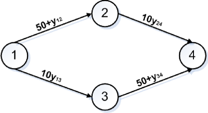
Figure 1: Case 1. $x_{124}=x_{134}=3$. Total time for each path is $T=83$ min.

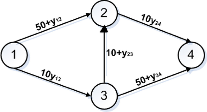
Figure 2: Case 2. $x_{124}=x_{1234}=x_{134}=2$. Total time for each path is $T=92$ min.

Example 2 (Nonuniqueness of the equilibrium; Shvetsov, 2010).
On Figure 3 the equilibrium flow distribution is shown, for all $x\in\left[{0,\;0.5}\right]$.

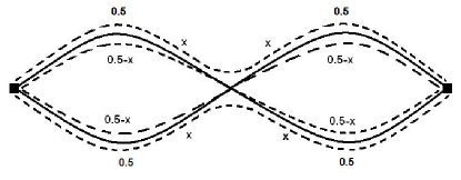
Figure 3: Nonuniqueness of the equilibrium.

Theorem 2

Let $T>0$ be sufficiently small, $\sum\limits_{n=1}^{\infty}{\gamma_{n}}=\infty,\sum\limits_{n=1}^{\infty}{\left({\gamma_{n}}\right)^{2}}<\infty$. Then $\Psi\left({\vec{x}\left(n\right)}\right)\mathrel{\mathop{\kern 0.0pt\longrightarrow}\limits_{n\to\infty}^{a.s.}}\Psi\left({\vec{x}^{\ast}}\right)$ and $\vec{x}\left(n\right)\mathrel{\mathop{\kern 0.0pt\longrightarrow}\limits_{n\to\infty}^{a.s.}}\vec{x}^{\ast}\left({\vec{x}\left(0\right)}\right).$ Note most of the elements of $\vec{x}^{\ast}\left({\vec{x}\left(0\right)}\right)$ can be equal to zero.

We should notice, that Theorem 2 is a refutation (in case of the considered dynamics) of the hypothesis [16]. It states that in the case of non-unique Nash-Wardrop equilibrium, the equilibrium is more likely to realize, and it is a solution of the following linear-enthropy programming problem

$$\sum\limits_{w\in W}{\sum\limits_{p\in P_{w}}{\left({x_{p}\ln\left({{x_{p}}\mathord{\left/{\vphantom{{x_{p}}{\left|{P_{w}}\right|}}}\right.\kern-1.2pt}{\left|{P_{w}}\right|}}\right)-x_{p}}\right)}}\to\mathop{\min}\limits_{\vec{x}\in X,\;\Theta\vec{x}=\vec{y}^{\ast}},$$

where $\vec{y}^{\ast}$ – is the unique solution of $V\left({\vec{y}}\right)=\sum\limits_{e\in E}{\int\limits_{0}^{y_{e}}{\tau_{e}\left(z\right)dz}}\to\min_{\vec{y}=\Theta\vec{x},\;\vec{x}\in X}$.

3 Sketch of the proof of the Theorem 1

Lemma 1

Let $f\left(w\right)=-T\ln w$, where $w\in\left({0,\;1}\right)$. $\alpha_{i}>0$ — are some randomly chosen, but fixed parameters; $w_{i}\in\left({0,\;1}\right)$. Let us consider functions

$$F_{0}\left({\vec{w}}\right)=\frac{\sum\limits_{i}{\alpha_{i}w_{i}f\left({w_{i}}\right)}}{\sum\limits_{i}{\alpha_{i}w_{i}}},\text{ and }F_{1}\left({\vec{w}}\right)=\frac{\sum\limits_{i}{\alpha_{i}f\left({w_{i}}\right)}}{\sum\limits_{i}{\alpha_{i}}}.$$

Then $F_{0}\left({\vec{w}}\right)\leq F_{1}\left({\vec{w}}\right)$, and the equality is attained only when

$$w_{1}=w_{2}=\ldots=w^{\ast}.$$

Proof.
The proof is based on the consequent usage of the inequality between harmonic mean and geometric mean and then Cauchy inequality. $\scriptstyle\blacksquare$

Lemma 2

For any $\vec{x}\left(n\right)\in X\colon\vec{x}\left(n\right)\neq\vec{x}^{\ast}$ holds the following inequality

$$\left\langle{\mathop{grad}\Psi\left(\vec{x}(n)\right),E\left[{\left.\vec{x}(n+1)-\vec{x}\left(n\right)\right|\vec{x}\left(n\right)}\right]}\right\rangle=\\ =\left\langle{\vec{G}\left(\vec{x}(n)\right),E\left[{\left.{\vec{x}(n+1)-\vec{x}(n)}\right|\vec{x}\left(n\right)}\right]}\right\rangle<0.$$ (4)

Proof.
Without restricting the generality, we can assume that $\forall\;p\in P\to x_{p}\left(n\right)\geq 1$. Then

$$\left\langle{\vec{G}\left({\vec{x}\left(n\right)}\right),\;E\left[{\left.{\vec{x}\left({n+1}\right)-\vec{x}\left(n\right)}\right|\vec{x}\left(n\right)}\right]}\right\rangle=$$

$$=\gamma_{n}\sum\limits_{w\in W}{d_{w}\left[{\frac{\sum\limits_{p\in P_{w}}{x_{p}\left(n\right)G_{p}\left({\vec{x}\left(n\right)}\right)\exp\left(-\cfrac{G_{p}(\vec{x}(n))}{T}\right)}}{\sum\limits_{p\in P_{w}}{x_{p}\left(n\right)\exp\left(-\cfrac{G_{p}(\vec{x}(n))}{T}\right)}}-\frac{\sum\limits_{p\in P_{w}}{G_{p}\left({\vec{x}\left(n\right)}\right)x_{p}\left(n\right)}}{\sum\limits_{p\in P_{w}}{x_{p}\left(n\right)}}}\right]}.$$

From Lemma 1 it follows that

$$\left\langle{\vec{G}\left({\vec{x}\left(n\right)}\right),E\left[{\left.{\vec{x}\left({n+1}\right)-\vec{x}\left(n\right)}\right|\vec{x}\left(n\right)}\right]}\right\rangle\leq 0.$$

And the equality can be attained only on the equilibrium vector $\vec{x}^{\ast}$, which can not be under considered hypothesis. $\scriptstyle\blacksquare$

Remark 1

Lemma 2 can be more specified. At some neighborhood of the equilibrium there exists $l>0$, such that

$$\left\langle{\vec{G}\left({\vec{x}\left(n\right)}\right),\;E\left[{\left.{\vec{x}\left({n+1}\right)-\vec{x}\left(n\right)}\right|\vec{x}\left(n\right)}\right]}\right\rangle\leq-l\gamma_{n}\cdot\left({\Psi\left({\vec{x}\left(n\right)}\right)-\Psi\left({\vec{x}^{\ast}}\right)}\right).$$

Also, with some reserves, we can change constraint $\vec{x}\left(n\right)\in X$ to $\vec{x}\left(n\right)\geq\vec{0}$.

Lemma 3 ([25], Chapter 2.2)

Let

$$\sum\limits_{n=1}^{\infty}{\gamma_{n}}=\infty,\quad\sum\limits_{n=1}^{\infty}{\left({\gamma_{n}}\right)^{2}}<\infty.$$

Then

$$\Psi\left({\vec{x}\left(n\right)}\right)\mathrel{\mathop{\kern 0.0pt\longrightarrow}\limits_{n\to\infty}^{\text{a.s.}}}\Psi\left({\vec{x}^{\ast}}\right)$$

and if the equilibrium is unique, then also

$$\vec{x}\left(n\right)\mathrel{\mathop{\kern 0.0pt\longrightarrow}\limits_{n\to\infty}^{\text{a.s.}}}\vec{x}^{\ast}.$$

Proof.
Lemma 2 and Theorem 1 from chapter 2.2 of [25] allow us to consider only the situation, when $\vec{x}\left(n\right)$ is close to $\vec{x}^{\ast}$. Then by Taylor formula we have:

$$E\left[{\left.{\Psi\left({\vec{x}\left({n+1}\right)}\right)}\right|\vec{x}\left(n\right)}\right]=\Psi\left(\vec{x}(n)\right)+$$

$$+\left\langle{\mbox{grad}\;\Psi\left({\vec{x}\left(n\right)}\right),\;E\left[{\left.{\vec{x}\left({n+1}\right)-\vec{x}\left(n\right)}\right|\vec{x}\left(n\right)}\right]}\right\rangle+{\rm O}\left({\left({\gamma_{n}}\right)^{2}}\right).$$

If we take mathematical expectations from both sides of this equality, we will get that there exists sufficiently large $C>0$, such that

$$E\left({\Psi\left({\vec{x}\left({n+1}\right)}\right)}\right)-\Psi\left({\vec{x}^{\ast}}\right)\leq\left({1-l\gamma_{n}}\right)\cdot\left({E\left({\Psi\left({\vec{x}\left(n\right)}\right)}\right)-\Psi\left({\vec{x}^{\ast}}\right)}\right)+C\cdot\left({\gamma_{n}}\right)^{2}.$$

From more general statement from [25] we get that

$$E\left({\Psi\left({\vec{x}\left(n\right)}\right)}\right)-\Psi\left({\vec{x}^{\ast}}\right)\mathrel{\mathop{\kern 0.0pt\longrightarrow}\limits_{n\to\infty}}0,$$

if

$$\sum\limits_{n=1}^{\infty}{\gamma_{n}}=\infty,\quad\sum\limits_{n=1}^{\infty}{\left({\gamma_{n}}\right)^{2}}<\infty.$$

From Kolmogorov inequality follows

$$P\left({\forall\;n\geq n_{0}\to\Psi\left({\vec{x}\left(n\right)}\right)-\Psi\left({\vec{x}^{\ast}}\right)\leq\varepsilon}\right)\geq$$

$$\geq 1-\varepsilon^{-1}\cdot\left({E\left({\Psi\left({\vec{x}\left({n_{0}}\right)}\right)-\Psi\left({\vec{x}^{\ast}}\right)}\right)+\sum\limits_{k=n_{0}}^{\infty}{\left({\gamma_{k}}\right)^{2}}}\right).$$

Which concludes the proof. $\scriptstyle\blacksquare$
In the end we will formulate a known result, which is in high correlation with the proved one.

Theorem 3

Let $T>0$. Then there $\exists\,C,\alpha>0\colon\forall\;N\in{\rm N}$

$$P\left({\Psi\left({\frac{1}{N}\sum\limits_{n=1}^{N}{\vec{x}\left(n\right)}}\right)-\Psi_{\min}\geq\frac{\Omega}{\sqrt{N}}}\right)\leq 2\exp\left({-C\cdot\Omega}\right),$$

where $\gamma=\frac{\alpha}{\sqrt{N}}$

Authors thank S.A. Avvakumov, I.B. Gnedkov, Y.V. Dorn, I.S. Menshikov, E.A. Nurminskiy, A.A. Shananin, V.I. Shvetsov and especially A.V. Gasnikov.

The work was supported by RFBR 10-01-00321-a, 11-01-00494-a 11-07-00162-a. The second author is partially supported by the Laboratory for Structural Methods of Data Analysis in Predictive Modeling, MIPT, RF government grant, ag. 11.G34.31.0073

References

• [1] Introduction to the mathematical modeling of traffic flow / Gasnikov A.V., Klenov S.L., Nurminskiy E.A., Kholodov Y.A., Shamray N.B.; with appendices M.L. Blank, E.V. Gasnikova, A.A. Zamyatin and V.A. Malyshev, A.V. Kolesnikov, A.M. Raigorodskiy, ed. A.V. Gasnikov. M.: MIPT, 2010. 361 p. (in Russian) http://zoneos.com/traffic/
• [2] Wilson A.G. (1970) Entropy in urban and regional modeling. Pion ltd., London.
• [3] Jaynes E.T. (1989) Papers on probability, statistics and statistical physics. Dordrecht: Kluwer Academic Publisher.
• [4] Popkov Yu.S. (1995) Macrosystems. Theory and its applications. Springer-Verlag.
• [5] Fang S.-C., Rajasekera J.R., Tsao H.-S. (1997) Entropy optimization and mathematical programming. Kluwer Academic Publishers.
• [6] Ledoux M.(2001) Concentration of measure phenomenon (2001). Providence, RI, Amer. Math. Soc., (Math. Surveys Monogr. V. 89).
• [7] Weidlich W.(2005) Sociodynamics. A systematic approach to mathematical modeling in social sciences. Harwood Academic Publishers, 2005.
• [8] Castellano C., Fortunato S., Loreto V.(2009) Statistical physics of social behavior // Review of modern physics, V. 81. 2009. P. 591-646. arXiv:0710.3256v2
• [9] Batishcheva Ya.G., Vedenyapin V.V. (2005) The second law of thermodynamics for chemical kinetics // Mat. Model., V. 17. 8. 2005. P. 106-110. (in Russian)
• [10] Malyshev V.A., Pirogov S.A. (2008) Reversibility and irreversibility in stochastic chemical kinetics // Uspekhi Mat. Nauk, V. 63. 1(379). 2008. P. 3-36.
• [11] Gasnikova E.V. (2009) Dual multiplicative algorithms for a problem of entropy-linear programming // Zh. Vychisl. Mat. Mat. Fiz., V. 49. . 3. 2009. P. 453-464.
• [12] Nesterov Yu., Nemirovskii A. (1985) Interior-point polynomial algorithms in convex programming. Philadelphia: SIAM, 1994.
• [13] Sheffi Y.(1985) Urban transportation networks: Equilibrium analysis with mathematical programming methods. N.J.: Prentice–Hall Inc., Englewood Cliffs, 1985.
• [14] Patriksson M. (1994) The traffic assignment problem. Models and methods. Utrecht Netherlands: VSP, 1994.
• [15] Steenbrink P.A. (1974) Optimization of transport networks. John Wiley & Sons 1974
• [16] Bar-Gera H. (1999) Origin-based algorithms for transportation network modeling. Univ. of Illinois at Chicago, 1999.
• [17] Foster D., Young P. (1990) Stochastic evolutionary game dynamics // Theoretical population biology. 1990. V. 38. 2.
• [18] Cressman R. (2003) Evolutionary game theory and extensive form games. Cambridge, Mass.: MIT Press, 2003.
• [19] Hofbauer J., Sigmund K. (2003) Evolutionary game dynamics // Bulletin of the AMS. 2003. V. 40. 4. P. 479–519.
• [20] McKelvey R. D., Palfrey T. R. (1998) Quantal response equilibria for extensive form games // Experimental economics. 1998. V. 1. P. 9–41.
• [21] Marsili M. (2001) Toy models of markets with heterogeneous interacting agents // e-print www.unifr.ch/econophysics/, 2001.
• [22] Fogel D. (2000) B. Evolutionary Computation: Towards a New Philosophy of Machine Intelligence. New York: IEEE Press, 2000.
• [23] Como G., Salva K., Acemoglu D., Dahleh M.A., Frazzoli E. (2011) Stability analysis of transportation networks with multiscale driver decisions // e-print arXiv:1101.2220v1.
• [24] Nesterov Yu. De Palma A. (2003) Stationary dynamic solutions in congested transportation networks: summary and perspectives // Networks and Spatial Economics, V. 3. 2003. P. 371-395.
• [25] Polyak B.T. (1987) Introduction to Optimization. Optimization Software Inc., 1987.
• [26] Juditsky A., Lan G., Nemirovskii A., Shapiro A. (2009) Stochastic approximation approach to stochastic programming // SIAM Journal on Optimization, 2009. V. 19. 4. P. 1574–1609. http://www2.isye.gatech.edu/$\sim$nemirovs/