The 3-Dimensional Distribution of Dust in NGC 891

Abstract

We produce three-dimensional Monte-Carlo radiative transfer models of the edge-on spiral galaxy NGC 891, a fast-rotating galaxy thought to be an analogue to the Milky Way. The models contain realistic spiral arms and a fractal distribution of clumpy dust. We fit our models to Hubble Space Telescope images corresponding to the B and I bands, using shapelet analysis and a genetic algorithm to generate 30 statistically best-fitting models. These models have a strong preference for spirality and clumpiness, with average face-on attenuation decreasing from 0.24(0.16) to 0.03(0.03) mag in the B(I) band between 0.5 and 2 radial scale-lengths. Most of the attenuation comes from small high-density clumps with low ($\lesssim$10%) filling factors. The fraction of dust in clumps is broadly consistent with results from fitting NGC 891’s spectral energy distribution. Because of scattering effects and the intermixed nature of the dust and starlight, attenuation is smaller and less wavelength-dependent than the integrated dust column-density. Our clumpy models typically have higher attenuation at low inclinations than previous radiative transfer models using smooth distributions of stars and dust, but similar attenuation at inclinations above 70^∘. At all inclinations most clumpy models have less attenuation than expected from previous estimates based on minimizing scatter in the Tully-Fisher relation. Mass-to-light ratios are higher and the intrinsic scatter in the Tully-Fisher relation is larger than previously expected for galaxies similar to NGC 891. The attenuation curve changes as a function of inclination, with $R_{B,B-I}=\frac{A_{B}}{E(B-I)}$ increasing by $\sim$0.75 from face-on to near-edge-on orientations.

1. Introduction

Understanding the 3D structure of dust is crucial for studies of spiral galaxies. In addition to detailing the complex structure of the ISM an accurate representation of dust is necessary to correct measurements of starlight. This is important for a variety of studies including e.g., the Tully-Fisher (TF) relation, where the behavior of the dust as a function of inclination is required to correct integrated photometry (Verheijen, 2001); constructing rotation curves of highly inclined galaxies, since attenuation can censor the rotation curve’s inner rise, leading to erroneous mass models (Matthews & Wood, 2001); correcting measurements of disk kinematics for the asymmetric amount of dust extinction above and below the disk of face-on spirals (Bershady et al., 2010a, b); and producing accurate radial surface-brightness profiles corrected for spurious broken-exponential morphologies caused by dust absorption (de Jong, 1996a). Spirals with inclinations at or near 90^∘ (known as edge-ons) provide the best information about the vertical structure of the dust, both because the corrections for viewing angle are small but also because the dust is projected into easy to see lanes that can attenuate the midplane by more than 10 mag in the optical (Kylafis & Bahcall, 1987). As a result edge-ons are an important component to our knowledge of dust structure. Separating the individual components of a dust-light mixture of unknown composition is a difficult endeavor, and is frequently done via radiative-transfer (RT) modeling.

Monte Carlo (MC) RT models, used in astrophysics since the 1970s (for a discussion of early models see Witt 1977), have been extensively employed to probe the structure of edge-on spirals. Recently, these models have come into prominent usage (e.g. Bianchi et al. 1996; Kuchinski et al. 1998; Matthews & Wood 2001; Baes et al. 2003, 2011), spurred by the need to precisely track multiple scatterings off dust grains. While costlier than the direct analytical approach of Kylafis & Bahcall (1987) in terms of CPU time, increases in processor speed and RAM limits coupled with rapidly dropping costs now allow detailed Monte Carlo models to be run on relatively short timescales. In addition, the current trend in high-performance computing is towards increased numbers of CPUs at slower clock speeds; this is also a benefit to Monte Carlo methods, as they are exceedingly well suited to parallelization and thrive in a distributed environment.

NGC 891 is the most studied nearby (d$\approx$9.5 Mpc) edge-on spiral galaxy in the universe. It is almost exactly edge-on ($i\approx 89.7^{\circ}$ (Xilouris et al., 1998)), with a rotation speed (212 km/s) similar to that of the Milky Way. Because the dust morphology of edge-ons appears to change significantly between galaxies with rotation speeds above and below 130 km sec^-1 (Dalcanton et al., 2004), comparing the Milky Way with other fast-rotating systems is especially relevant. NGC 891 is also one of the first galaxies discovered to have high-latitude HI, a discovery prompted by observations of high-latitude HI in our own galaxy (Gerard, 1973; Strong, 1978). Indeed, NGC 891’s potential as an analogue of the Milky Way is what aroused much of the early interest in this extragalactic system (Bahcall, 1983; van der Kruit, 1984). More recently, evidence for a strong two-armed spiral pattern like that seen in grand design spirals such as M51 has emerged based on asymmetry in H$\alpha$ and B band emission (Kamphuis et al., 2007; Xilouris et al., 1998). NGC 891 appears to have a bar (Garcia-Burillo & Guelin, 1995) as well as a nearby companion (UGC 1807, Mapelli et al. 2008), both of which dramatically increase the likelihood of the aforementioned grand design pattern being real (Elmegreen & Elmegreen, 1982).

NGC 891 is also known for its abundance of high-latitude dust and complex dust substructure. Given the significant high-latitude HI found in NGC 891, it is not surprising to also find dust away from the midplane. Howk & Savage (1997) used unsharp masks to study individual high-latitude dust clumps in NGC 891, and later found evidence that these extended substructures may be common to most spirals (Howk & Savage, 1999). If high-latitude dust caused by star-formation induced outflows is indeed abundant in spiral galaxies, it would act as a foreground screen preferentially over the star-forming spiral arms, increasing the apparent optical depth in the arms without increasing total dust content. While unsharp masks are very useful for enhancing clumpy substructure the masking process destroys quantitative information about the clumps. Therefore, a new procedure for highlighting the dust that preserves this information is needed.

Because there are some indicators of spirality and significant extraplanar dust component, NGC 891 is a clear example of the need for advanced 3D modeling which takes into account these features. Indeed, studies attempting to use smooth, axisymmetric models on NGC 891 have had significant difficulty in fitting the data due to the asymmetry in blue light. Xilouris et al. (1998) split the galaxy in half and used an infinitely long thin disk of stellar emission to reconcile the left and right hand sides of NGC 891 in the B and V bands, while additional dust and light components have been required by smooth models to fit NGC 891’s mid-infrared emission (Popescu et al., 2000; Bianchi, 2008). Some groups have added clumpy/non-axisymmetric structure to RT models of edge-on spirals (e.g. Kuchinski et al. 1998; Mihos et al. 1999; Matthews & Wood 2001; Misiriotis & Bianchi 2002; Bianchi 2008); however they restrict their analysis to a small range of clumpy models, with dust modeled by hand or based on results for the Milky Way.

In this work we quantitatively fit the first RT models to include both dust clumping and realistic spirality to F450W and F814W Hubble images of NGC 891. These RT models resemble real spiral galaxies from any inclination angle, allowing us to make accurate inferences about the dust properties of galaxies like NGC 891 as seen at all inclinations. In Section 2 we present the archival data used in this work and our methods of analysis. In Section 3 we discuss the parameter space of our model, our fitting algorithm, and our fitness metric. We present our results, including a brief post-facto analysis of our shapelet-based fitness metric, in Section 4. In Section 5 we discuss the photometric properties of our models and compare them to the literature. Finally, in Section 6, we present our concluding remarks.

2. Observational Constraints

2.1. Data

We downloaded HST WFPC2 images of the central region of NGC 891 from the Hubble Legacy Archive in the F450W and F814W bandpasses (hereafter referred to a B and I band, respectively). For S/N per pixel $\approx$ 10 the data go down to a limiting mag of $\sim$18.5 STMAG mag arcsec^-2 for both B and I bands. The images were rotated in order to make the galaxy midplane horizontal, and then smoothed to a resolution of $\sim$0.9” (roughly 42 pc at the adopted distance of 9.5 Mpc) to match the resolution of the models. Due to the large size of the galaxy on the WFPC2 images the sky had been oversubtracted in the reduced, archival data. We corrected the sky subtraction while scaling and centering the images by comparing the data to smooth, axisymmetric RT models constructed exactly from the B and I band parameters given in Popescu et al. (2000). This procedure was iterative: starting from a guess of the offsets, we computed a linear least-squares fit between individual pixels from the model images and their analogues in the shifted data frames. The best-fitting shift is the one required to center the image, while the slope and y-offset of the best fit are the flux calibration and background offset, respectively. We then masked out bright foreground stars and background galaxies from the images. These masks were homogenized between the B and I bands, then preserved so we could identically mask all of our models before fitting them to the data.

2.2. Metrics of non-axisymmetric systems with clumpy dust distributions

The aim of this study is to determine the clumpy and non-axisymmetric distribution of star-light and dust in NGC 891. To do so, we introduce two new metrics to characterize the data and our models. These metrics are designed to evaluate the performance of these models in matching the data compared to axisymmetric models with smooth star-light and dust distributions. First, we motivate the concept of attenuation, from which we construct a differential index of the attenuation relative to a smooth model. This index allows us to leverage the most important observable differences between smooth and clumpy distributions of dust. Second, with the use of models with clumpy distributions of dust, it is no longer tractable to find a model that looks identical to the data (as done in all prior smooth model analyses). We apply a method from the literature for making orthogonal decompositions of two-dimensional light distributions. These characterizations are used to statistically compare and contrast the observed and modeled differential attenuation maps.

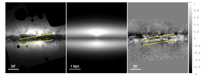
Figure 1.— Demonstration of the $\Delta A_{I}^{\rm e}$ map. Left: smoothed I band HST image of NGC 891. Center: smooth model from Popescu et al. (2000). Right: $\Delta A_{I}^{\rm e}$ map. The color-map shows the differential attenuation in mag. The clumpy, non axisymmetric structures have been highlighed by the $\Delta A_{I}^{\rm e}$ map while smooth structure (e.g. high-latitude bulge light) has been removed. Of special note is a line of increased attenuation running across the center of the galaxy but at a non-zero angle to the midplane (bracketed by dashed yellow lines). This could be indicative of a warped outer spiral arm.

2.2.1 Differential Attenuation Maps

Whenever dust grains are mixed with a distribution of stellar emissivity the traditional notion of dust as a purely foreground screen no longer applies; instead what we observe for systems such as galaxies is the attenuation $A_{\lambda}^{\rm e}$ at wavelength $\lambda$. The attenuation can be defined in analogy to the foreground extinction, $A_{\lambda}$, by the ratio of the observed or modeled line-of-sight flux in the presence of dust ($F_{\lambda}$) to the line-of-sight flux (of a model) in the absence of dust ($F_{\lambda}^{0}$):

$$A_{\lambda}^{\rm e}\ \equiv\ -2.5\log\left(\frac{F_{\lambda}}{F_{\lambda}^{0}}\right).$$ (1)

In general, $A_{\lambda}^{\rm e}$ is dependent on the underlying distribution of emissivity, absorption, and scattering. Consequently, $A_{\lambda}^{\rm e}$ is not related simply to the dust optical depth, and hence cannot be used to derive directly the underlying dust column density.

Previous radiative transfer modeling of galaxies which fit models to images (e.g., Xilouris et al. 1998) have constrained smooth distributions of stars and dust by fitting directly to the observed, two-dimensional light distribution at different wavelengths. To first order, our clumpy dust models must reproduce this basic two-dimensional light distribution on average. However, if we try to fit clumpy models directly to the observed light distribution, the solution will be degenerate since there will be many combinations of clumpy dust and star-light that either (a) will result in the same observed intensity along a given line of sight; or (b) will result in similar net deviations (in a $\chi^{2}$ sense) from the observed data. Because of these degeneracies (whereby a wide range of astrophysically distinct models yield similar goodness of fit to the data), fitting clumpy models to the observed light distribution is not particularly meaningful. Instead, what is meaningful is to determine the similarity of the statistical deviations of the light-distributions of the data and models with respect to some fiducial distribution. Since we are interested in understanding the importance of clumpy dust, the best fiducial distribution is a model consisting of a smooth light and dust distribution that best approximates the data.

Hence, instead of directly comparing our clumpy models to the data, we use differential attenuation ($\Delta A_{\lambda}^{\rm e}$) maps. Similar to the attenuation $A_{\lambda}^{\rm e}$, these images are created by taking the ratio of the observed flux or non-axisymmetric model flux to the flux distribution of a fiducial, axisymmetric, smooth model:

$$\Delta A_{\lambda}^{\rm e}\ \equiv\ -2.5\log\left(\frac{F_{\lambda}}{F_{\lambda,s}}\right),$$ (2)

where $F_{\lambda,s}$ is the flux from the fiducial model. The fiducial model is comprised of starlight and dust, and can be parameterized in terms of its own attenuation $A_{\lambda,s}^{\rm e}$ and the same model without dust ($F_{\lambda,s}^{0}$):

$$F_{\lambda,s}=F_{\lambda,s}^{0}\,10^{-0.4A_{\lambda,s}^{\rm e}}.$$ (3)

The differential attenuation can then be expressed as a function of the underlying stellar distributions and the attenuation of the data/clumpy model and the smooth model:

$$\Delta A_{\lambda}^{\rm e}=-2.5\log\left(\frac{F_{\lambda}^{0}}{F_{\lambda,s}^{0}}\right)+A_{\lambda}^{\rm e}-A_{\lambda,s}^{\rm e}.$$ (4)

If the fiducial model’s light distribution, integrated along the line-of-sight in the absence of dust, is a reasonable approximation to the astrophysical object or clumpy model (also in the absence of dust), then the first term is negligible. In general the choice of fiducial model is relatively unimportant as long as it is held constant for the entire analysis since the mismatch can be treated as a pedestal value to $\Delta A_{\lambda}^{\rm e}$. We choose the axisymmetric, smooth model described in Xilouris et al. (1998) and Table 1 of Popescu et al. (2000) as our fiducial. The observed $\Delta A_{\lambda}^{\rm e}$ and the ingredients are shown for NGC 891 in Figure 1. The left panel shows a smoothed I band HST image, the center panel shows an image of the smooth model created using our MC RT software, and the right panel shows the ratio of the other two panels — the $\Delta A_{\lambda}^{\rm e}$ map.

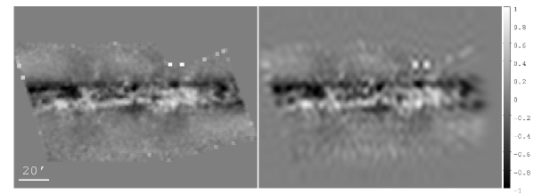
Figure 2.— Sample shapelet reconstruction of the observed I band $\Delta A_{\lambda}^{\rm e}$ map. Left: $\Delta A_{I}^{\rm e}$ map. Right: reconstruction of $\Delta A_{I}^{\rm e}$ map using 50 orders in x and 25 orders in y. Color-bar indicates differential attenuation, in mag. The shapelet reconstruction effectively smooths the image with a boxcar of radius one pixel. Going to higher orders does not significantly improve this resolution, as it is impossible to perfectly reconstruct an image without using infinite orders.

It is important to note two things about the $\Delta A_{\lambda}^{\rm e}$ maps. First, these maps do not represent the true attenuation because the axisymmetric models include a smooth dust disk: The $\Delta A_{\lambda}^{\rm e}$ map is really showing the excess or dearth of attenuation due to non-axisymmetric components (such as spiral arms and clumps). For instance, the $\Delta A_{I}^{\rm e}$ map (and to a lesser extent $\Delta A_{B}^{\rm e}$ map) shows a long, thin structure running across the middle of the galaxy with greater than expected attenuation (highlighted in Figure 1). This feature is angled off of the midplane and resembles what would be expected from a warped outer spiral arm. A warp in NGC 891 would help explain its significant extraplanar gas emission from ionized and neutral gas (Rand et al., 1990; Swaters et al., 1997; Oosterloo et al., 2007), although Keppel et al. (1991) indicate that a warp is unlikely. By highlighting these structures the $\Delta A_{\lambda\,eff}$ maps focus our model fitness parameters on the higher order structure that we are searching to constrain.

Second, the $\Delta A_{\lambda}^{\rm e}$ maps’ ability to highlight dust substructure is similar to the unsharp masks used by Howk & Savage (1999); however, by using the attenuation instead of an unsharp mask we are able to bring out the substructure without destroying the quantitative information in the image (a byproduct of any algorithm involving smoothing). This is a significant advantage over unsharp masking because it allows us to compute quantitative values that can be directly compared to physical models.

2.2.2 Shapelet Analysis

The problem of identifying ways to characterize clumpy models and compare them meaningfully to data has been taken up in the literature. However, the solution to date has been to turn away from modeling the observed spatial distribution of light (as done in all prior smooth model analyses), and towards fitting the spectral energy distribution (SED). The latter essentially compresses all the model images into a single dimension, which can then be fit using a simple $\chi^{2}$ analysis. However this method throws away all spatial information, which is essential for testing physical models where stellar emission, absorption, scattering, and thermal re-emission are not necessarily co-spatial processes. By ignoring spatial information modelers also run the risk of finding false minima, simulations that fit the SED but do not look like real galaxies (for an example of this see Bianchi 2008).

Another approach to constraining clumpy models which does not throw away spatial information, is to construct a suitable statistical descriptor of the galaxy image structure (here we use $\Delta A_{\lambda}^{\rm e}$ for the structure image). One must find a way to measure the statistical properties of the image that is able to equate two systems with the same underlying distribution of structure. The human eye is very good at this task, and “by-eye” image fitting has had some success (e.g., Matthews & Wood 2001). However, in order to create rigorous and well-constrained clumpy models a computerized, quantitative tool to measure image structure is needed. As a first step in this new direction we employ shapelet analysis to generate model fitnesses.

Shapelet analysis, first described by Refregier (2003), is a method for decomposing an image into orthogonal basis functions using weighted Hermite polynomials. A cousin of wavelets, shapelets are optimized for the more circular features generally found in astronomy. The shapelet methodology creates orthogonal basis functions based on Hermite polynomials:

$$\phi_{n}(x)=\frac{H_{n}(x)e^{-x^{2}/2}}{\sqrt{2^{n}n!\sqrt{\pi}}}$$ (5)

where $H_{n}$ is the Hermite polynomial of order of positive integer $n$. These 1D basis functions are combined to produce a dimensional 2D basis function:

$$B_{n_{1},n_{2}}(x_{1},x_{2};\beta)=\beta^{-1}\phi_{n_{1}}\left(\frac{x_{1}}{\beta}\right)\phi_{n_{2}}\left(\frac{x_{2}}{\beta}\right).$$ (6)

Here $\beta$ is a constant scaling factor used to scale the size of the shapelets. The number of counts in an image pixel is then equal to the infinite sum of the shapelet basis functions multiplied by the shapelet coefficients, given by

$$f_{n_{1},n_{2}}=\int\int f(x_{1},x_{2})B_{n_{1},n_{2}}(x_{1},x_{2};\beta)\,\mathrm{d}x_{1}\,\mathrm{d}x_{2},$$ (7)

where $f(x_{1},x_{2})$ are the counts for a given pixel. For a much more thorough description see Refregier (2003). Traditionally shapelets have been used to model spatially small galaxies at a low number of fourier modes (e.g. Kelly & McKay 2004; Massey et al. 2004; and Kuijken 2006). We are trying to deconstruct objects on size scales ranging from a few pixels (dust clumps) to the size of the image (the bulge and disk) and therefore must go to much higher order in shapelet space. We choose to go to 50th order along the major axis and 25th order along the minor axis, based on a comparison of sample reconstructions of the smoothed HST images. Going to these higher orders allows us to capture much of the structural detail. Exploring such high order shapelets is possible because shapelet deconvolution is a relatively efficient procedure, especially compared to the time it takes to run our RT models. Additionally, parts of the process are parallelizable (e.g. computing shapelet coefficients), a fact we take full advantage of wherever possible. A sample reconstruction using the selected orders is shown in Figures 2 and 3. Reconstructing the image to less than infinite orders imposes a penalty on image resolution; the reconstructed image appears slightly smoothed, roughly equivalent to boxcar-smoothing the image with a radius of one pixel. The pixelization of the image, pixel-to-pixel noise, and the rapidly increasing computational expense inhibit the use of higher orders. Even though the shapelets we use are designed for circular objects (cf. Bosch 2010) we find that they are able to accurately reproduce the oblong features of edge-on spirals as well as the clumpy dust.

3. Modeling

Including both spirality and dust clumping adds many free parameters to the RT models. Because many of these parameters are new to the modeling literature, we cannot simply adopt values based on results from previous studies. Consequently, our parameter space is very large and so we employ a genetic algorithm to maximize our efficiency at finding ’good’ solutions. Such an algorithm is well suited to comparing a statistical goodness-of-fit constructed from the amplitude distribution of the shapelet decomposition of $\Delta A_{\lambda}^{\rm e}$.

3.1. The model

We use the 3D scattered light Monte Carlo RT model developed by K. Wood, which has been used in a variety of different astrophysical environments (for example see Wood et al. 1996; Wood & Jones 1997; Wood et al. 1999; Wood & Loeb 2000; Matthews & Wood 2001; and Sankrit & Wood 2001). We will summarize the relevant details here; for a full description of the code see Wood & Reynolds (1999).

The Monte Carlo model tracks individual packets of photons through a model consisting of a 3D Cartesian grid, where each cell has a fixed dust density. The packets are transmitted, absorbed, or scattered in a given cell based on the results of random numbers weighted by the physical properties of the dust and its density in that cell. The temperature of the dust is not tracked; our scattered-light model does not re-emit absorbed photons — once they are absorbed, they are terminated. We ignored the effects of dust emission in this work, although UV-excited extended red emission (the so-called ERE: Perrin et al. 1995; Pierini et al. 2002) might contribute modestly to the I-band light of NGC 891 at high latitudes. The advantage of using a scattered-light RT code is computational — models can be run faster and with higher resolution than if we used RT software which tracked absorption and re-emission of dust.

Our model employs a forced first scattering algorithm, where all photon packets are scattered at least once (Witt, 1977). We also use a ’peeling off’ formula (Yusef-Zadeh et al., 1984), which directs a fraction of each photon packet’s light toward the observer regardless of the packet’s nominal direction. Both of these modifications allow us to achieve a higher S/N for a given number of emitted photon packets with minimal loss in accuracy.

We use a grid of 1000x1000x500 cells, which is mapped to a spatial volume of 40x40x20 kpc. This gives us a resolution of $\sim$0.9” at a distance of 9.5 Mpc. Because our simulations are at such high resolution, we have parallelized the Monte Carlo code to run on a 12-core processor.

3.1.1 Stellar Emissivity

As described below, we include multiple components to characterize both the stellar emissivity and dust density, using a very similar parameterization to that of Popescu et al. (2000) and Misiriotis et al. (2000).

We model the stellar emission as a smooth spatial distribution with non-axisymmetric components in the form of spiral arms. Further, emission is treated completely separately for each band to take into account the change in dominant stellar population as a function of wavelength. This is in line with the models of Xilouris et al. (1999) and Popescu et al. (2000), among others. The emissivity is governed by the following equation:

$$L(R,z)=L_{B,0}e^{-7.67B^{0.25}}B^{-0.875}+L_{D,0}e^{-\frac{R}{h_{r}}-\frac{z}{h_{z}}}\xi.$$ (8)

The first part of this expression describes an elliptical de Vaucouleurs bulge, where $L_{B,0}$ is the bulge emissivity of the central cell and $B$ is an intermediate quantity containing information about the bulge effective radius $R_{e}$, semimajor axis $a$, and semiminor axis $b$:

$$B=\frac{\sqrt{R^{2}+z^{2}(a/b)^{2}}}{R_{e}}.$$ (9)

The second part of equation (8) controls a double-exponential disk, where $L_{D,0}$ is the disk emissivity of the central cell, and $h_{r}$ and $h_{z}$ are the scale-length and -height, respectively. The third component, $\xi$, is the logarithmic spiral disk perturbation, and expands into

$$\xi= 1-w+\prod_{n=2,n+2}^{N}\frac{n}{n-1}w\sin^{N}\times$$

$$\left(\frac{\ln(\sqrt{x^{2}+y^{2}})}{\tan(p)}-\tan^{-1}\left(\frac{y}{x}\right)+45^{\circ}\right)$$ (10)

where $x$ and $y$ are the cartesian coordinates, $w$ is the fraction of light (or dust, see §3.1.2) entrained in the arms, and $p$ is the pitch angle. Equation 10 is a modified form of logarithmic spirality in Misiriotis et al. (2000); the main changes are the inclusion of the even-numbered exponent $N$ and the fixing of the spiral arms at two. The asymmetry of H$\alpha$, 60 $\mu$m, and CO emission point to NGC 891 being a classical grand design spiral (Kamphuis et al., 2007; Garcia-Burillo et al., 1992; Xilouris et al., 1998), justifying the use of only two arms. In the Misiriotis spirality formulation the arms and interarm regions have equal size. Schweizer (1976) showed that this was not the case; the ratio between arms to interarm regions is closer to 0.2 for grand design spirals. Exponentiating the sine part of the function allows us to (coarsely) adjust the arm-interarm ratio; $N=10$ roughly corresponds to the correct ratio. We have chosen the form of the spirality so that if $N=2$ it reduces to the equation in Misiriotis et al. (2000). The product in front of the equation ensures that the spiral perturbation does not change the total emissivity.

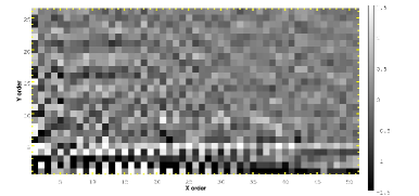
Figure 3.— Shapelet coefficients of the observed I band $\Delta A_{\lambda}^{\rm e}$ map. Horizontal orders are along the x-axis, while vertical orders are along the y-axis. Lower orders are on the left and bottom, respectively. The color-bar shows the amplitude of the shapelet coefficients.

3.1.2 Dust

We populate our models with the same dust geometry in all wavebands, as the dust density distribution is independent of wavelength. The RT software takes as an input the total dust+gas density, so we note that the assumption that the dust follows the gas is implicit in our models. The dust density distribution is assumed to be very similar to that of the starlight in the disk on large scales, e.g. there is no dust bulge, and hence

$$\rho_{d}(R,z)=\rho_{0,d}e^{-\frac{R}{h_{r}}-\frac{z}{h_{z}}}\xi\,\digamma(R,z),$$ (11)

where $\rho_{0,d}$ represents the dust+gas disk density of the central cell. The scale length and height can be different than those of the stars, $\xi$ is the same basic formula as for emissivity (Equation 10) but with (potentially) different values for $w$, and $\digamma$ represents a clumping modifier. Clumpiness is governed by a fractal algorithm based on the distribution of molecular dust in the Milky Way (Elmegreen, 1997) and is detailed in Mathis et al. (2002). Because the fractal algorithm is designed to mimic dust substructure on much smaller scales than we will probe, it is not known a priori how well it can reproduce the large, chimney-like structures usually taken as evidence for large scale outflows due to e.g., supernovae. In the ideal case we would use a dynamical, turbulent model of the ISM computed from hydrodynamical simulations (like those created by Joung & Mac Low (2006)), but using these models on galactic length scales is currently computationally infeasible. The fractal algorithm is computationally efficient and can produce a wide range of substructure.

For the physical properties of the dust grains we choose values consistent with the diffuse interstellar medium of the Milky Way, based on the dust model of Mathis et al. (1977) as computed by White (1979). The adopted parameters are fairly consistent with prior efforts to fit RT models to images (e.g. Xilouris et al. 1999). More recent studies (e.g. Draine 2003) have found somewhat different dust properties, although we note that determining these parameters can be difficult (Lewis et al. 2009 and references therein). Three parameters govern the dust physics relevant to our models: $\chi$, the total (dust+gas) opacity; $a$, the albedo; and $g$, the scattering asymmetry parameter. For the B band we adopt $\chi=286$ cm² g^-1, $a=0.54$, and $g=0.48$. In I we use $\chi=105$ cm² g^-1, $a=0.49$, and $g=0.29$. These values for $\chi$ correspond to an $R_{V}=3.27$, marginally larger than the value of $R_{V}$ for a screen of dust in the Milky Way (Cardelli et al., 1989). The same dust model is used for both the smooth and the clumpy components of the dust distribution.

3.1.3 Free and Fixed Parameters

We hold the bulge parameters constant using values from the smooth model of Popescu et al. (2000) (L${}_{Bulge,B}=12\times 10^{30}$ erg s^-1 pc^-3 str^-1, L${}_{Bulge,I}=2.23\times 10^{30}$ erg s^-1 pc^-3 str^-1, b/a_B = 0.6, b/a_I=0.54, R_e,B=1.12 kpc, and R_e,I=1.97 kpc), under the assumption that the bulge should be relatively smooth and axisymmetric and is well characterized from light outside the midplane where dust absorption is minimized. This assumption is not perfect. For instance NGC 891 is known to have a bar (Garcia-Burillo & Guelin, 1995). We choose not to fit a bar to save CPU expense in this large parameter space since our main area of interest lies in the disk and not the bulge/bar.

We expect that the only change to the scale-lengths of the starlight from those reported for smooth exponential models will be due to azimuthal variations in the spiral pattern; therefore any deviation from the Popescu et al. (2000) values of the scale-length ($h_{r,B}=5.67$ kpc, $h_{r,I}=4.93$ kpc) in one band will be well correlated with deviations in the other, giving a single free $h_{r,B}$ parameter. However, while any randomly generated models follow this rule, we allow the scale-lengths to change just like the other free parameters as the models ’breed’ with each other. Therefore the scale-lengths in both bands are generally highly correlated, but not perfectly so. We leave the central emissivity $L_{D,B,0}$ and $L_{D,I,0}$ and the scale-heights $h_{z,B}$ and $h_{z,I}$ as free parameters because while they are largely insensitive to spiral perturbations (Misiriotis et al., 2000) they are likely to be sensitive to dust clumpiness.

Misiriotis et al. (2000) show that with the addition of spirality $L_{D,0}$ and $h_{r}$ can vary up to about 30% (for large offsets between stellar and dust arms). We allow $L_{D,B,0}$, $L_{D,I,0}$, to vary between 0.67 and 2 times the values given by Popescu et al. (2000) and $h_{r,B}$ to vary between 0.5 and 1.5 times the literature value. As the effect of clumpiness on scale-heights is uncertain we allow $h_{z,B}$ and $h_{z,I}$ to vary by up to a factor of two from values in the literature. (For reference, Popescu et al. (2000) use $L_{D,B,0}=2.66\times 10^{27}$ erg s^-1 pc^-3 str^-1, $L_{D,I,0}=3.44\times 10^{27}$ erg s^-1 pc^-3 str^-1, $h_{z,B}=0.43$ kpc, and $h_{z,I}=0.38$ kpc).

Table 1Free Parameters

Parameter name	Symbol	Lower limit	Upper limit	Median	10%	90%	Unit
Central disk emissivity (B band)	$L_{D,B,0}$	1.78x1027	5.35x1027	2.69x1027	2.04x1027	4.03x1027	erg s-1 pc-3 str-1
Central disk emissivity (I band)	$L_{D,I,0}$	2.3x1027	6.9x1027	3.39x1027	2.74x1027	4.65x1027	erg s-1 pc-3 str-1
Emission scale-length	$h_{r,B}$	2.84	8.51	6.23	4.52	7.88	kpc
Emission scale-height (B band)	$h_{z,B}$	0.22	0.86	0.46	0.37	0.59	kpc
Emission scale-height (I band)	$h_{z,I}$	0.19	0.76	0.45	0.33	0.60	kpc
Central dust+gas density	$\rho_{0,d}$	1.24$\times$10-4	0.31	1.6x10-2	6.3x10-3	8.8x10-2	g cm-2 kpc-1
Dust scale-length	$h_{r,\rho}$	3.99	11.96	6.41	4.44	9.34	kpc
Dust scale-height	$h_{z,\rho}$	0.135	0.54	0.24	0.16	0.34	kpc
B band spiral perturbation strength	$w_{B}$	0	1	0.56	8.7x10-2	0.71	-
Dust spiral perturbation strength	$w_{\rho}$	0	1	0.49	0.20	0.74	-
Pitch angle	$p$	10	30	20.50	15.17	26.6	degrees
Number of initial fractal clumps	$N_{1}$	50	200	129	75	163	-
Smooth fraction (dust)	$f_{\rho}$	0	0.8	0.42	0.15	0.59	-

The dust parameters are generally treated very similarly to their analogues in stellar emissivity. Changes to the scale-length of the dust $h_{r,\rho}$ appear to be correlated with changes to the scale length of the stellar emission (Misiriotis et al., 2000); however this correlation appears to break down for small pitch angles and so we leave $h_{r,\rho}$ to vary to within 50% of literature value (7.97 kpc). The dust vertical scale height can vary by a factor of two from the Popescu et al. (2000) value of 0.27 kpc. Because $\rho_{0,d}$ is a strong function of clumpiness (Misiriotis & Bianchi, 2002) we allow it to vary up to 50 times literature value (we choose a fiducial $\rho_{0,d}$ of 0.0062 g cm^-2 kpc^-1, a compromise between the B and I band values of Popescu et al. (2000)); while we do not expect such large discrepancies from the literature in $\rho_{0,d}$ (or indeed, any of our free parameters) the ability of the genetic algorithm to quickly find local minima allows us to be very ambitious in selecting our parameter space.

We allow the dust perturbation strength ($w_{d}$) and the B band perturbation strength ($w_{B}$) to vary freely; Schweizer (1976) found that the ratio of arm strength between bands similar to B and I was about 1.2, and we use this value to set $w_{I}$. The pitch angle $p$ of the stellar spiral arms is also a free parameter, allowed to vary between 5 and 30 degrees, while the pitch angle of the dust lag is fixed to the emission so that the dust arms always are 5 degrees apart from the stellar arms. Both the pitch angle range and dust offset angle are based on studies of face-on spiral galaxies by Kennicutt (1981). We fix the position angle $PA$ (corresponding to the $\phi$ direction of a cylindrical coordinate system where the r and z directions are parallel to the radius and vertical extent, respectively, of the galaxy) because our data only covers the innermost part of NGC 891 and is therefore unlikely to be sensitive to changes in $PA$, although we do test each model for both spiral orientations (left-handed or right-handed). Finally, we allow the full range of spiral perturbation strengths (0 to 1) for both stars and dust.

The major parameters of the fractal algorithm are the fractal dimension $D$, governing the size scale of the clumps; $N_{1}$, the number of clumps; and $1-f_{\rho}$, the fraction of the total dust density trapped in the clumps. We follow Indebetouw et al. (2006) and set $D=2.6$: while this is larger than the value used by Elmegreen (1997) it is within the observational limits found by Elmegreen & Falgarone (1996) and gives more “fluffy” clouds (Indebetouw et al. 2006; for a schematic illustration of the fractal algorithm see Figure 4 of Wood et al. 2005). Small values of $N_{1}$ lead to a few, isolated, clouds while large values correspond to smoother, more uniform, structures. We therefore allow $N_{1}$ to vary freely between 50 and 200, which (despite the aforementioned fact that the fractal algorithm is designed for smaller structures) we experimentally find produces realistic looking clumpy distributions. All subsequent casts control the size and filling factor of individual clumps and are set to 32, which we have found produces rich structure down to our resolution limit without significant added CPU expense.

After determining the distribution of clumpy regions we set the fraction of dust in the clumps. The smooth fraction $f_{\rho}$ is a free parameter which is allowed to vary between 0 and 80% of the total dust mass, observing that smooth fractions larger than 80% tend to be indistinguishable from the entirely smooth models which are uninteresting to probe in this study. The ranges of all the free parameters used in the models is shown in Table 1.

3.1.4 Additional Test Models

With a total of 13 free parameters, we also wanted to understand how well constrained our model was. To that end, we also ran a set of models with a significantly reduced parameter space. We fixed both the scale-length and scale-height for the stars and the dust at the values of our fiducial model ($h_{r,B}=5.67$ kpc, $h_{r,I}=4.93$ kpc, $h_{z,B}=0.43$ kpc, $h_{z,I}=0.38$ kpc, $h_{r,\rho}=7.97$ kpc, and $h_{z,\rho}=0.27$ kpc), and set the stellar spiral perturbation strength $w_{B}$ (0.4) and pitch angle $p$ (15^∘) equivalent to values consistent with Sb galaxies (Schweizer, 1976). This leaves us with a total of only six free parameters for our ‘constrained’ models.

Additionally, we examined our decision to fix the $PA$ by running a subset of 8 models with the full set of 13 free parameters as well as varying the $PA$ between 0 and 180 degrees. These 8 models are heareafter referred to as the ‘free-PA’ models. We investigate how changing our free parameters in this way affects our resulting models in §4.1.1.

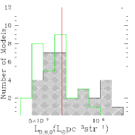
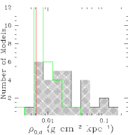
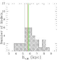
Figure 4.— Histograms of central B band emissivity (left), central dust+gas density (middle), and B band scale-length (right) for the 30 best-fitting models. Gray shaded histograms are for the unrestricted sample, while green empty histograms show the restricted sample. Red vertical lines denote values from the simple smooth model of Popescu et al. (2000).

3.2. Genetic Algorithm

Our total number of free parameters is 13. This presents an algorithmical challenge, as it would take prohibitively long to do a brute-force search of parameter space. What is required, then, is an algorithm that can efficiently search through a parameter space without deeply probing regions with only poor fits to the data. Multiple approaches exist for this problem, but we choose a genetic algorithm both for its simplicity and efficiency.

Genetic algorithms take their inspiration from the evolutionary principles of natural selection. A population of models is created, then their fitnesses are computed. The model with the best fitness is cloned, and passed on unchanged to the next generation. Individual models then pseudo-randomly pair off to ’breed’ to populate the next generation with the same number of models, where models with better fitnesses are statistically more likely to breed more often. The gene pool is refreshed either through the occasional influx of new models or through random mutations of existing models, thereby avoiding population stagnation.

If the fitness criterion is adequate at discriminating between ‘good’ and ‘bad’ models a genetic algorithm will rapidly converge to a local minimum. Due to the continuous mixing of parameters and introduction of new ones the genetic algorithm is capable of skipping lightly over poor local minima and quickly finding a relatively deep local minima. After this point increasing the number of generations has little effect, as the minimum is too deep for mutations or breeding with new models to easily climb out and find a better one. At this point the genetic algorithm becomes little better than a Monte Carlo analysis. Therefore, the optimal way to run a genetic algorithm is to determine roughly how long it takes for the algorithm to converge on a good minimum (usually through running empirical test models), then run multiple iterations of the algorithm only up to that number of generations to map out the deep local minima.

Because the genetic algorithm spends little time searching through bad regions of parameter space, adding unconstrainable free parameters to the model does not significantly increase computing time. Therefore, while we may not expect all 13 of our free parameters to be well-constrained (e.g. the spirality parameters) including them does not strongly affect run-time or ‘pollute’ well-constrained parameters.

Our genetic algorithm is based on that of Howley et al. (2008), who used it to study the orbit of NGC 205, a satellite of M31. Our algorithm is very similar to theirs; the reader is referred there for more detail. Our modifications are small: we use eight models in each generation instead of five, we replace all but the best model with random ones every eight generations to prevent population stagnation, and we use a single fitness indicator instead of trying to combine several as they do.

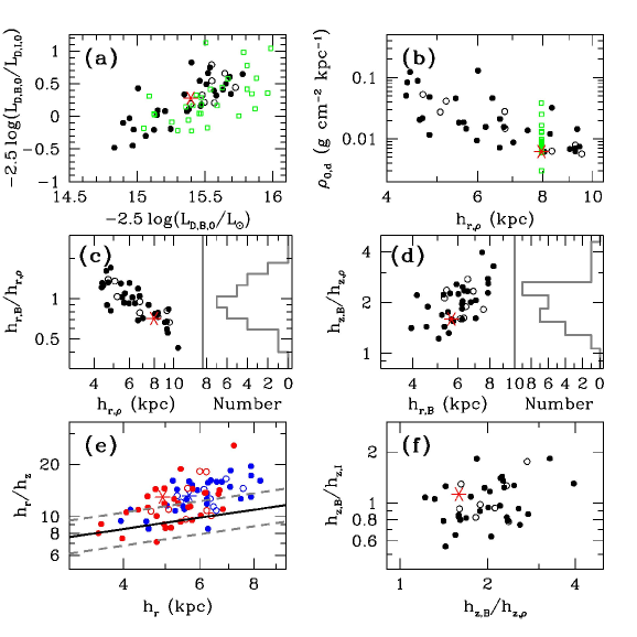
Figure 5.— Correlations between free parameters shown in Figure 4 and other axisymmetric parameters for our best fitting clumpy models and the simple smooth model of Popescu et al. (2000). (a) Central emissivity color as a function of B band central emissivity. (b) Central dust+gas density versus dut scale-length. (c) Ratio of the B band to dust scale-lengths versus the dust scale-length. (d) Ratio of the B band and dust scale-heights against the B band scale-length. (e) Ratio of scale-length to scale-height for the B (blue) and I (red) bands against the B and I band scale-length. (f) Ratio of B to I band scale-heights as a function of the ratio of B band to dust scale-heights. Black dots denote clumpy models, red stars denote the simple smooth model, open black circles denote the subset of clumpy models with variable position angles, and open green squares (in a and b) denote the models with restricted parameter space. When necessary, blue denotes the B band and red denotes the I band. The thick black line shows the empirical correlation and 1$\sigma$ scatter between scale-length and scale-height from Bershady et al. (2010b).

3.3. Fitness

In our approach, shapelet analysis produces a map of the contribution to the reconstructed $\Delta A_{\lambda}^{\rm e}$ image at all possible combinations of orders. However, we do not use this map to model $\Delta A_{\lambda}^{\rm e}$ images for comparison on a pixel-by-pixel basis with the observed $\Delta A_{\lambda}^{\rm e}$ image. This is because the detailed spatial variations of $\Delta A_{\lambda}^{\rm e}$ are dependent on random variables (in reality due to the stochastic nature of star formation; in the models by construction). Consequently a direct comparison in image-space is swamped by the mis-match in random structure. In contrast, however, the relative amplitudes of shapelet coefficients do capture the power in structures at different spatial frequencies, and hence provide a good statistical descriptor of the physical distribution of emission, absorption, and scattering. Therefore we use the shapelet coefficients directly to compute a fitness statistic:

$$\mathcal{F}=\sum_{n=0,m=0}^{N,M}\left|C(n,m)_{model}-C(n,m)_{data}\right|$$ (12)

where $n$ and $m$ are the shapelet orders, and $C(n,m)$ is the shapelet coefficient magnitude at order n,m. Equal weights are given to each coefficient, and by not adding in quadrature we prevent the largest coefficients (usually in the lowest orders, governing the large-scale structure) from dominating the fitness. The fitnesses of each filter are added in quadrature, and the geometric orientation with the best combined fitness is used in the genetic algorithm. Using this merit function the genetic algorithm essentially matches each coefficient to the same absolute tolerance, automatically adjusting the tolerance from large to small as it improves the fit over the course of several generations.

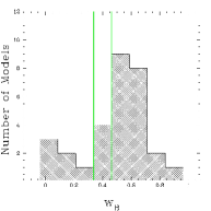
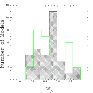
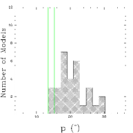
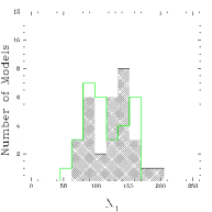
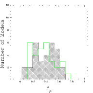
Figure 6.— Histograms of non-axisymmetric parameters for the best-fitting clumpy models for unrestricted sample (gray shading) and restricted sample (green lines). Top left: B band spiral perturbation strength. Top middle: dust+gas spiral perturbation strength. Top right: pitch angle. Bottom left: number of fractal clumps. Bottom right: smooth dust fraction.

4. Results

The HST images only cover the inner $\sim$9 kpc of NGC 891 so we only output model images that cover a corresponding area. This results in images that are $230\times 230$ pixels, where 1 pixel = 1 projected cell. We choose to simulate a much larger volume than we need so that we can produce images showing the full model galaxy with the same random clumping behavior (because of the semi-random nature of the clumps changing the grid volume would change the clump distribution, even when holding the random seed constant). However, in our genetic algorithm we only allow photons to be emitted along the central 10 kpc of the disk (5 kpc in radius) in both the y and z directions (where x is along the line of sight) which allows us to obtain higher S/N with fewer photons. Empirically, we determine that a model with 5 million photons emitted with the above restriction produces acceptable images.

On a 2.93 GHz 12-core machine each band for NGC 891 takes approximately 2-3 minutes to run for a single set of model parameters, which is by far the time-limiting step in the genetic algorithm. We find that the genetic algorithm has largely settled into a local minimum after 50 8-model generations, so we truncate the algorithm there. Even with only 50 generations each run of the genetic algorithm takes about a day, so while it would be ideal to use more generations per run (Howley et al. 2008 use 1000) we opt to limit the number of generations and therefore have time for more runs. Even so, time constraints limit our final sample to only 30 runs. Each run contains up to 351 distinct models ($>10^{4}$ models total), but we only select the best model from each run for our analysis. While 30 runs does not allow us to make the detailed analysis of parameters found in Howley et al. (2008), it does allow us to make a broader survey of the parameter space. For our parameter space tests, we used 8 runs for the models with variable $PA$ added to the normal 13 free parameters and a full 30 runs for the constrained set of models containing only 6 free parameters.

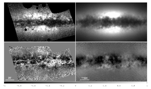
Figure 7.— Comparison of one of our best fitting non-axisymmetric RT models with data for the B band. Top left: smooth HST image. Top right: model image. Bottom left: $\Delta A_{B}^{\rm e}$ map for data. Bottom right: $\Delta A_{B}^{\rm e}$ map for model. The color-bar shows the differential magnitudes of the $\Delta A_{B}^{\rm e}$ maps.

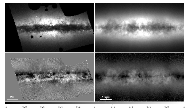
Figure 8.— Same as Figure 7, but for the I band.

4.1. Best Fitting Models

In Figures 4—6 we show histograms and plots of the free parameters in our clumpy models, as well as (where appropriate) our ‘free-$PA$’ and ‘constrained’ models. Figure 4 contains histograms of the central B band emissivity $L_{D,B,0}$, central dust+gas density $\rho_{0,d}$, and B band scale-length $h_{r,B}$ overplotted with the appropriate values of the smooth, single-disk model of Popescu et al. (2000) which we used as the basis for our clumpy models. While there is significant scatter in all three parameters, on average our models prefer slightly lower central B band emissivities, slightly higher central dust densities, and B band scale-lengths roughly equivalent to those of the smooth model.

There is significant scatter for most of the individual parameters. While initially this may seem to indicate that our models are unconstrained, a closer inspection reveals that the scatter for individual parameters hides deeper correlations between multiple parameters, indicating that there are several strong joint constraints.

In Figure 5 we plot several noticeable relationships between the parameters shown in Figure 4 and the other emissivity and scale parameters. Values for the Popescu et al. (2000) model are shown with red stars, or blue (B band) and red (I band) stars when data from both bands are plotted simultaneously. In all cases the values for the smooth model fall within the bivariate distributions of our clumpy models. For reference, the data from the ‘free-PA’ and ‘constrained’ subsets of models are shown (where appropriate) as open circles and open squares, respectively.

First, there is a correlation between redder central emissivities and fainter central B band emissivity (Figure 5a), but the correlation is in excess of what would arise for a constant I band emissivity. In other words, model disks with fainter central B band emissivity tend to have relatively higher central I band emissivity.

Figure 5b shows that as the radial size of the dust disk is inversely proportional to the central dust density: larger dust disks have more diffuse dust. In terms of the relative size scales of the dust and stellar disks, the B band radial scale-length is comparable to the dust scale-length (Figure 5c), with a mean ratio of $\sim$1. However, as the size of the dust disk increases the relative size of the B band stellar disk decreases, with the largest dust disks having $\frac{h_{r,B}}{h_{r,\rho}}\approx 0.5$. The stellar vertical scale-heights of our clumpy models are typically twice that of the dust, with a positive correlation between B band radial scale-length and the ratio of B band scale-height to the dust scale-height. (Figure 5d). Hence the dust oblateness is roughly half that of the stars. The oblateness of the stellar disk in the B (blue) and I (red) bands increases modestly with the stellar radial scale-length (Figure 5e), departing somewhat from the empirical relationship between oblateness and scale-length derived by Bershady et al. (2010b). The stellar disks are slightly larger in the B band than the I band, and both bands are somewhat flatter than typical galaxies of comparable size and Hubble type. We find little degeneracy in the models between intrinsic vertical color gradients in the stellar emissivity and varying scale-heights of dust to stars: In Figure 5f there is little correlation between the ratio of the B and I band scale-heights and the ratio of the B band scale-height to the dust scale-height (bottom right).

Finally, we plot histograms of parameters related to the spirality and clumpiness in Figure 6. While there is significant scatter, fully two-thirds of our models have at least 50% of their B band emission and dust density tied up in spiral arms with a preferred pitch angle of about 20^∘. However, we also find that our models don’t show a strong preference for the direction of spirality (left- or right-handedness). It therefore seems likely that the spirality is not well constrained in or simulations, and as a result we do not present a thorough analysis of the spirality parameters.

Our models do show a strong preference towards having a significant amount of dust entrained in clumps; 27 of the 30 best fitting models have smooth dust fractions $f_{\rho}$ smaller than 0.6, which means that 90% of the best fitting models have $\geq 40\%$ of their total dust mass arranged into clumps. The median clumpiness fraction $1-f_{\rho}$ is 58%, which is a factor of only 1.2 smaller than current clumpy estimates fitting to the energy balance solely through SEDs Bianchi & Xilouris (2011). The number of clumps (governed by $N_{1}$) is generally fairly large, with a slight preference for $N_{1}\geq 125$. These parameters combine to give our models significant amounts of non-axisymmetric structure.

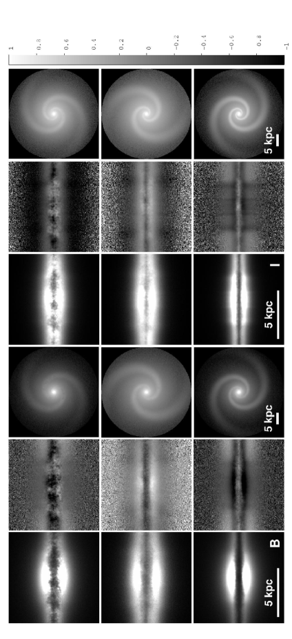
Figure 9.— Representative sample of the best fitting clumpy models. From left: edge-on B band images, edge-on $\Delta A_{B}^{\rm e}$ maps, face-on B band images, edge-on I band images, edge-on $\Delta A_{I}^{\rm e}$ maps, face-on I band images. Color-bar denotes $\Delta A_{\lambda}^{\rm e}$ for B and I bands, in mag. Each model was fit both as a clockwise and counter-clockwise rotating spiral. While the orientations with the best fits are shown here, generally the difference in fitness between orientations was small. Additionally, some of the models (even with the same orientation) appear to have different $PA$s, however this is an illusion caused by the varying pitch angles as well as the self-similar nature of the logarithmic spirality.

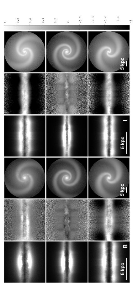
Figure 9.— Continued.

4.1.1 Consistency Checks

The subset of models with variable position angle converge at $PA$s varying between 61 and 170^∘, with a median value of 109^∘. The lack of models with $PA$s between 0 and 60^∘ is intriguing, as it indicates that even with the restricted image coverage of HST our models may have some sensitivity to spiral parameters. However, as seen in Figure 5, the ‘free-PA’ models do not have different physical parameters from the full sample, indicating that our assumption of a fixed $PA$ does not significantly affect our results.

The ‘constrained’ sample, however, does appear to have a distribution of central luminosities that is, on average, fainter than for the full sample. While initially surprising, on closer inspection this discrepancy is a function of fixing the scale-lengths of the models: The literature value for $h_{r,\rho}$ is larger than most of the fitted scale-lengths of the full sample (Figure 5c). This drives the central dust density down (Figure 5b), which also lowers the central luminosities. It is worth noting that our full, unrestricted sample appears to produce a tighter correlation between color and luminosity (Figure 5a) than the ‘constrained’ sample. This, along with the lack of significant systematic differences between the ‘constrained’ and full samples for any of the non-axisymmetric parameters (Figure 6) leads us to conclude that our full models are as well-constrained as the ‘constrained’ sample and a better match to the observational data.

4.2. Analysis of the shapelet coefficients

Because of the large variations in the parameters of our best fitting models, we check to make sure the shapelet coefficients are properly optimizing our models. In Figures 7 and 8 we show the best fitting model out of all the runs, compared to the HST images. Our model is optimizing towards a plausible representation for the global light and dust distribution of NGC 891.

To investigate how well our shapelet-amplitude statistic performs as a fitness indicator (and to get a better overall view of the range of models selected by the genetic algorithm) we show a sample (20%) of the best-fitting clumpy models in Figure 9. The images are representative of variation seen in the 30 models from all the genetic algorithm runs. Overall it is clear that the shapelet-derived fitness in the $\Delta A_{\lambda}^{\rm e}$ images is doing an adequate job of picking models that globally resemble NGC 891. The luminous bumps in $\Delta A_{\lambda}^{\rm e}$ seen to the left and right of the bulge in some of the models (see e.g., the bottom panels of Figure 9) are due to the spiral arms. These images also show that our formalism can create models with significant clumpy, non-asymmetric structure. However, even the clumpiest-looking models in our sample lack the high-z tendrils often described as vertically oriented “chimney”-like structures. This discrepancy may indicate that the fractal algorithm is unable to produce the necessary substructure to mimic those seen in massive, edge-on galaxies, and highlights the need for physically motivated dynamical models for the ISM (such as Wood et al. 2010).

While the dust chimneys seen in images of NGC 891 and other edge-on galaxies are visually striking, their effect on the global photometric properties of galaxies is likely to be small. The chimneys’ apparent stochasticity and likely origin in large outflows implies that properly modeling them would not significantly change the free parameters such as dust mass, scale-height, or central emissivities. Similarly, they are likely to be very localized, foreground structures and as such should play a relatively minimal role in determining total attenuation corrections at all inclinations.

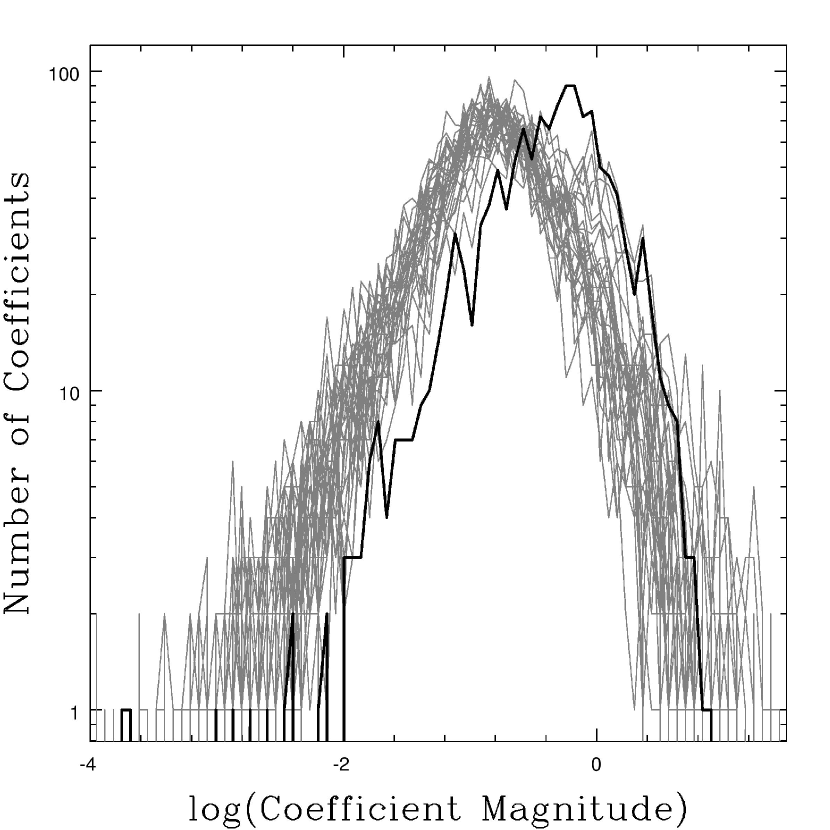
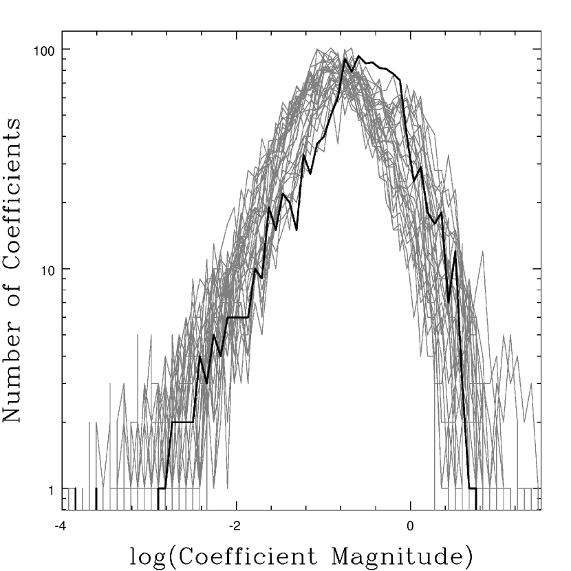
Figure 10.— Histograms of shapelet coefficient magnitudes that reproduce the observed (black) and best fitting clumpy models’ (gray) $\Delta A_{\lambda}^{\rm e}$ maps. Left: B band. Right: I band.

In an attempt to gain more insight into how our algorithm matches and mismatches the observed complex dust structures, we have examined the shapelet amplitude distributions of the 30 best-fitting models. We plot histograms of the magnitudes of the shapelet coefficients at all x,y orders for the HST images and our models in Figure 10. The peak of the coefficient histograms of the clumpy models occurs at a lower coefficient magnitude than the peak for the reconstruction of the HST data in both B and I, although the peaks are less separated in the I band — possibly due to the B band’s increased sensitivity to dust attenuation. The clumpy model reconstructions in both bands also have more coefficients at the largest magnitudes. The lack of medium-magnitude coefficients in the clumpy models means that most of the power lies in just a few coefficients with large magnitudes, producing less rich substructure than seen in reconstructions of the data.

We also investigated the even vs. odd distribution of the shapelet coefficients, by comparing the sums of the coefficient magnitudes in the even orders with those in the odd orders. This was prompted by inspection of shapelet coefficient maps like the one shown in Figure 3, which has a sawtooth-like pattern of coefficients. We find an even-to-odd ratio of $\sim$1 for both observed bands. Our models, however, tend towards much higher ratios, which can be seen in Figure 11. This trend is apparent when coefficients that are even in the x (horizontal) or y (vertical) dimension are used, and is another indicator that it may be possible to further exploit the shapelet analysis to find more realistic models.

5. Discussion

5.1. Face-on appearance of the models

The goal of this work was to create physically realistic RT models that would resemble real galaxies at any inclination, something that the current literature on axisymmetric structure and/or hand-added clumpiness has difficulty doing. It is clear from the results of our genetic algorithm that our spiral structure formalism is able to reproduce the general edge-on appearance of NGC 891, which is not a surprise based on the results of Misiriotis et al. (2000). But how realistic do our best-fitting models appear at other inclinations?

To answer this question we reran our RT code, using the same inputs for all 30 of our best-fitting models (even down to the same random seed) but changing the inclination angle to zero and allowing photons to be emitted from the outer parts of the disk. A representative sample of the results is shown in columns three and six of Figure 9. Virtually all of the models have prominent spiral features, although there is disagreement in the handedness of the spirality. Given the restricted radial range of the data, it is unsurprising that direction of the spiral arms is poorly constrained; while we display the orientation with the best fitness most models had comparable fitnesses for spiral arms in both directions. There is also some variation in pitch angle, but for a given handedness it is relatively consistent, giving a fairly uniform look to many of these models. It is likely that at least some of the variation in spiral parameters is due to the restricted areal coverage of the HST images; using a lower-resolution image of the full galaxy might yield stronger constraints.

Whether or not the spiral parameters are well constrained, our prescription for spirality works fairly well, producing realistic-looking spiral arms. Our models produce face-on images with much brighter spiral arms compared to the bulge than the ’typical spiral galaxy’ model of Misiriotis et al. (2000). Compressing our spiral arms by a factor of five greatly increases their relative brightness for the same axisymmetric model parameters, preventing our models with larger pitch angles from looking like the oblong blobs in the top panel of their Figure 1.

5.2. Face-on extinction and attenuation

5.2.1 Attenuation

The general effect of compressing the dust into lagging spiral arms is to create lanes of absorption along the inner edges of the luminous arms. For the models with smoother dust this can be difficult to see in Figure 9. Images of the face-on attenuation, $A_{\lambda}^{\rm e}$, of the models from Figure 9 are shown in the first and third columns of Figure 12 for the B and I bands, respectively. These attenuation maps are computed by comparing models with dust to models with no dust, computed using identical parameters. Red regions are areas of high attenuation, while blue indicates regions with no attenuation. Most ($\sim$70%) of the models show a maximum face-on $A_{\lambda}^{\rm e}<0.6$ mag in both bands. Of the few models with $A_{B}^{\rm e}>1$ mag, none have a peak attenuation $\gtrsim$2 mag, while the peak attenuation in the I band is $\sim$1.5 mag. All models show very low attenuation at radii larger than $\sim$1 $h_{r}$, even for models with strong spiral features at larger radii between the center of the galaxy and the observation direction in edge-on orientation (off the bottom of the face-on images). Areas of peak attenuation are highly confined to the spiral arms: the average filling factor of the clumpy models for $A_{\lambda}^{\rm e}\geq 0.5$ mag at 0.5, 1, and 2 $h_{r}$ is, respectively, 12.1, 5.2, and 0.4% in the B band and 5.5, 2.5, and 0.1% in the I band. Filling factors at other thresholds are given in Table 2.

We measured the average face-on attenuation to be $A_{B}^{\rm e}=0.24$, 0.15, and 0.03 mag and $A_{I}^{\rm e}=0.16$, 0.10, and 0.03 at 0.5, 1, and 2 scale-lengths respectively. In analogy to $R_{V}$ with a typical value of 3.1 measured for foreground dust screens in the Milky Way, we define an attenuation curve parameter $R_{B,B-I}$ as

$$R_{B,B-I}=\frac{A_{B}}{E(B-I)}.$$ (13)

With this definition, a foreground screen of Milky Way-type dust has $R_{B,B-I}=1.56$ (Cardelli et al., 1989), and empirical estimates of the attenuation of star forming galaxies yields $R_{B,B-I}=1.76$ (Calzetti et al., 2000). In contrast the $R_{B,B-I}$ values for our clumpy models are much larger ($R_{B,B-I}=3$ at 0.5 and 1 $h_{r}$) and become undefined (positively infinite) at larger radii. In other words, the attenuation is much grayer in our clumpy models than for a foreground screen, and appears to become grayer with increasing radius (due to scattering). The increase in the ratio of total to selective extinction for clumpy models relative to smooth models was noted for spherical systems by (for example) Witt & Gordon (1996) and Witt & Gordon (2000), as well as in more realistic models of disk galaxies by Pierini et al. (2004).

Table 2Filling Factors for Attenuation

		Filling Factor Threshold (mag)
Band	Radius ($h_{r,B}$)	$<0.1$	$<0.3$	$<0.5$	$<1.0$	$<3.0$
B	0.5	47.4%	23.8%	12.1%	2.5%	0.0%
I	0.5	34.1%	11.1%	5.5%	1.0%	0.0%
B	1.0	34.9%	11.3%	5.2%	1.2%	0.0%
I	1.0	22.1%	5.0%	2.5%	0.3%	0.0%
B	2.0	13.3%	1.4%	0.4%	0.0%	0.0%
I	2.0	15.7%	0.9%	0.1%	0.0%	0.0%

5.2.2 Extinction as a foreground screen

We are also able to compute the face-on dust optical depth of our clumpy models. The extinction from this optical depth (here called $A_{\lambda}$) is very different than the attenuation: While $A_{\lambda}^{\rm e}$ is the attenuation of the admixture of dust and stars in a galaxy the optical depth governs the extinction on objects behind the galaxy, where the dust functions exclusively as a foreground screen. Foreground extinction images are shown in the second and fourth columns of Figure 12. We find that this foreground screen extinction is significantly higher than the attenuation, with an average $A_{\lambda}$ at 0.5, 1, and 2 $h_{r}$ of 2.35, 1.35, and 0.45 mag in the B band and 0.91, 0.55, and 0.22 mag in the I band. In magnitudes, the scaling between $A_{B}$ and $A_{B}^{\rm e}$ is roughly a factor of 11, while between $A_{I}$ and $A_{I}^{\rm e}$ there is a magnitude scaling of roughly a factor of 6. The difference in these two scale factors imply that the foreground screen is less gray, as expected. We find foreground screen values of $R_{B,B-I}\sim 1.8\pm 0.2$, comparable to the Calzetti et al. 1994 attenuation curve. The foreground screen extinction is much higher than $A_{\lambda}^{\rm e}$ due to a combination of scattering and the overlapping nature of the stellar emission and dust, a discrepancy which has been noted previously (e.g. Pierini et al. 2004). To confirm this we ran a version of one of our clumpy models with the dust offset to 5 kpc in front of the galaxy and scattering turned off, which produced a ’pseudo foreground extinction’ image very similar to the actual foreground screen extinction. Removing the scattering even without offsetting the dust was enough to increase $A_{\lambda}^{\rm e}$ by about 0.5 mag in both B and I bands, a large enough amount to make some regions change from optically thin to thick.

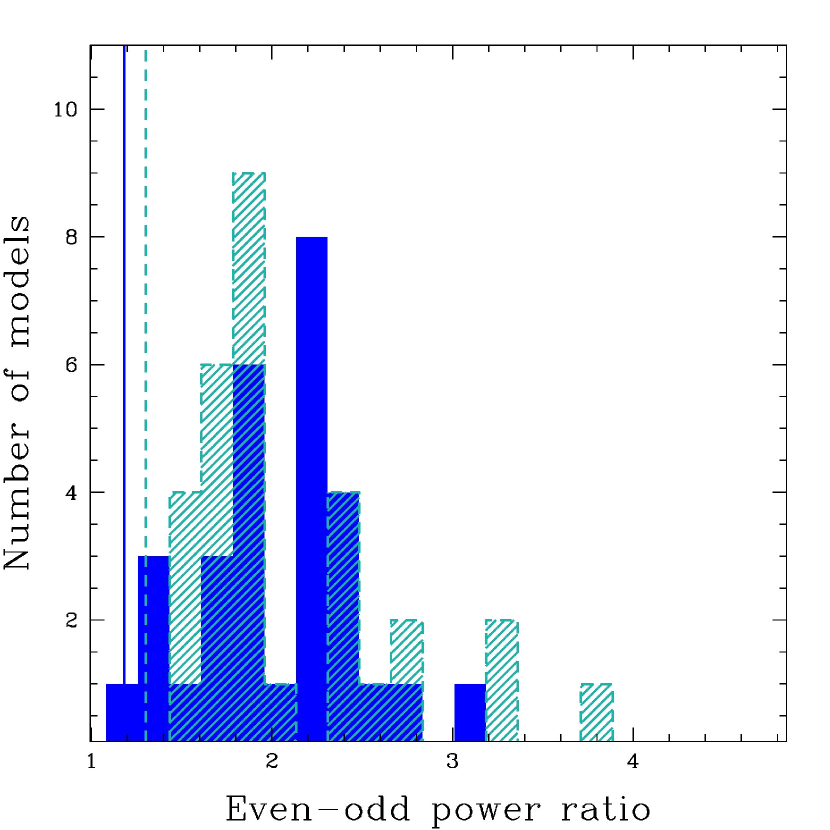
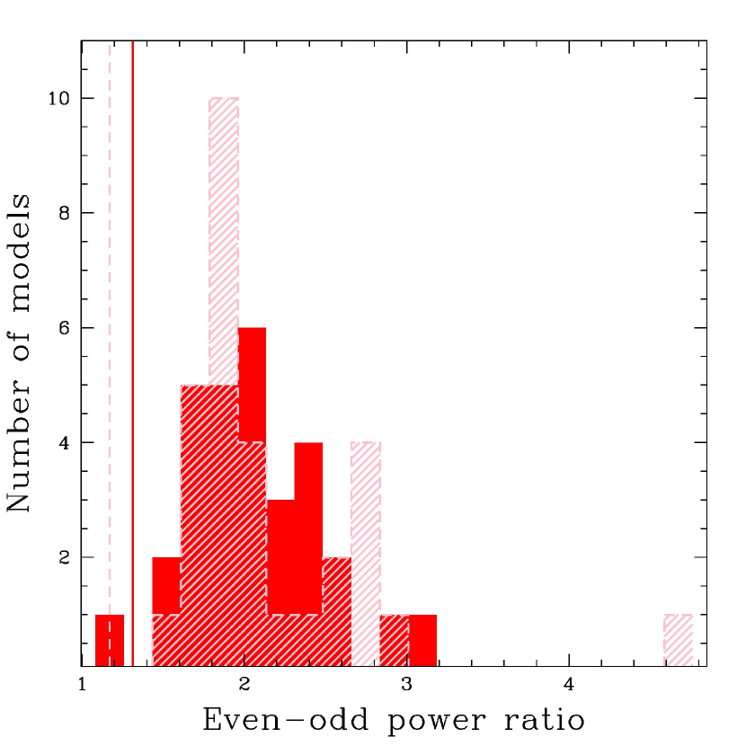
Figure 11.— Distribution of the total power ratio in even and odd shaplet coefficients that reproduce $\Delta A_{\lambda}^{\rm e}$ of the 30 best-fitting models. The power ratio is computed by summing the magnitude of every even coefficient and dividing by the summed magnitude of odd coefficients. Left panel: B band. Right panel: I band. Solid histograms denote ratios computed by selecting coefficients at even x (horizontal) values, while the dashed histograms show ratios for even y (vertical) coefficients. Solid and dashed vertical lines show the ratios selecting for x and y even coefficients, respectively, for the $\Delta A_{\lambda}^{\rm e}$ constructed from the observed images of NGC 891.

Table 3Filling Factors for Screen Extinction

		Filling Factor Threshold (mag)
Band	Radius ($h_{r,B}$)	$<0.1$	$<0.3$	$<0.5$	$<1.0$	$<3.0$
B	0.5	99.1%	92.7%	82.6%	58.8%	18.7%
I	0.5	95.2%	68.4%	50.2&	23.4%	4.9%
B	1.0	98.3%	84.2%	65.1%	37.4%	8.4%
I	1.0	89.5%	51.3%	30.6%	11.4%	2.1%
B	2.0	89.7%	45.1%	27.2%	9.4%	0.9%
I	2.0	60.6%	19.2%	8.6%	2.3%	0.1%

We can compare these results to measurements in the literature for other spirals. Using the HyperLEDA database (Paturel et al., 2003) and assuming D=9.5 Mpc we find $R_{25}\approx 18$ kpc and therefore $h_{r}\approx 0.3R_{25}$. At 0.3 $R_{25}$ Holwerda et al. (2005) find an average $A_{I}$ at this radius of roughly 0.5-1 mag (see the top left panel of their Figure 7), in agreement with our results. However, while we also find that the largest source of dust column-density comes from the spiral arms, Holwerda et al. (2005) report $A_{I}$ of $\sim$1 mag at one scale-length. Our models contain less dust extinction between the arms. For example, at one scale-length the I band filling factor for extinction $\geq$0.5 mag in our models is only 31%. On the other hand, White et al. (2000) and Domingue et al. (2000) find similar values for the foreground screen extinction in spiral arms in the B and I bands (albeit with a spread of $\gtrsim$1 mag for both bands) but interarm extinction values of $0<A<1.4$ mag, with most galaxies in their sample having interarm extinction closer to zero. Holwerda et al. (2009) report optical depths almost entirely lower than 0.5 from B to I band in the outer regions of a backlit spiral. These results are consistent with our models, where we find the average filling factor for foreground screen extinction with a threshold of 0.3 mag is 84.2% and 51.3% at 1 scale-length in the B and I bands, respectively (additional optical depth values and filling factors for our models of NGC 891 are given in Table 3). Our models also consistently predict large central face-on optical depths, with values ranging from $\sim$2.5 to $>$4 in the B band. However, Kuchinski et al. (1998) find central optical depths of 0.5-2.0 in the V band, which for Milky Way-type dust is equivalent to $\tau_{B}\approx$0.7-2.7. This discrepancy is likely due to the inability of optical models to see to the center of the galaxy.

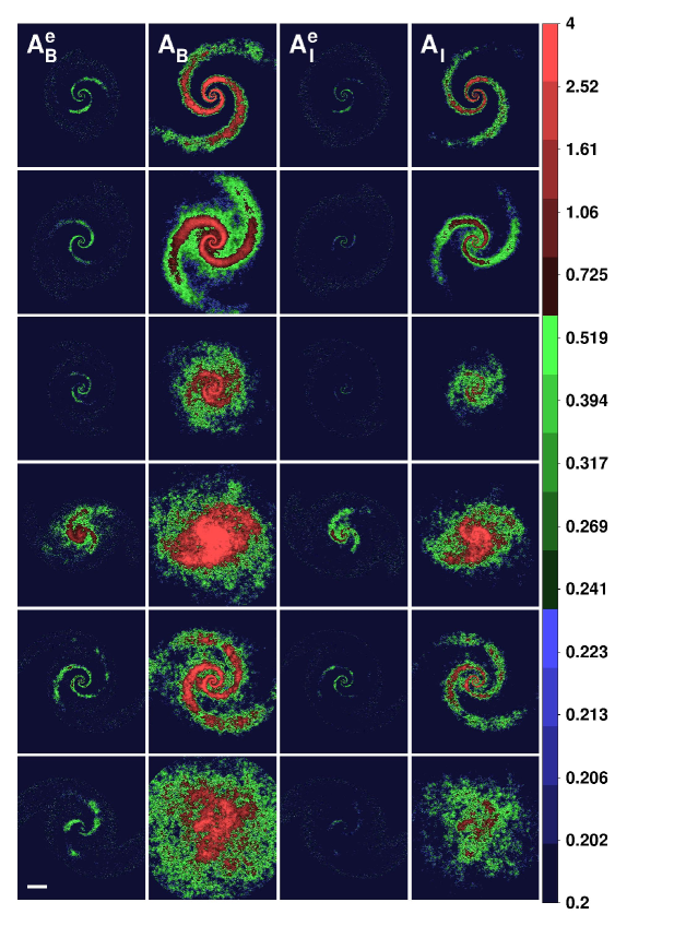
Figure 12.— Face-on attenuation maps for the models shown in Figure 9. From left: B band attenuation, B band foreground screen extinction, I band attenuation, I band foreground screen extinction. The white bar in the lower left represents a distance of 5 kpc, while the color scale is in mag.

An inspection of Figure 12 shows a wide range of dust column-density morphology (and therefore foreground screen extinction) but a much smaller range of appearances for the attenuation. For example, in rows two and six, the model attenuation looks fairly similar, with low levels of patchy attenuation tracing out narrow spiral arms. In contrast, the foreground screen maps are vastly different: The dust in row two is confined largely to prominent spiral arms while the dust in row six shows little coherent structure. These degeneracies imply that estimates of the attenuation based on measurements of a galaxy’s extinction as a foreground screen are not well constrained — unsurprising given the complex interplay between dust and starlight in these galaxies. As important, measurements of galaxies’ dust content observed as a foreground screen (e.g., White et al. (2000), Holwerda et al. (2005)) yield estimates of attenuation that are many times too large and not gray enough.

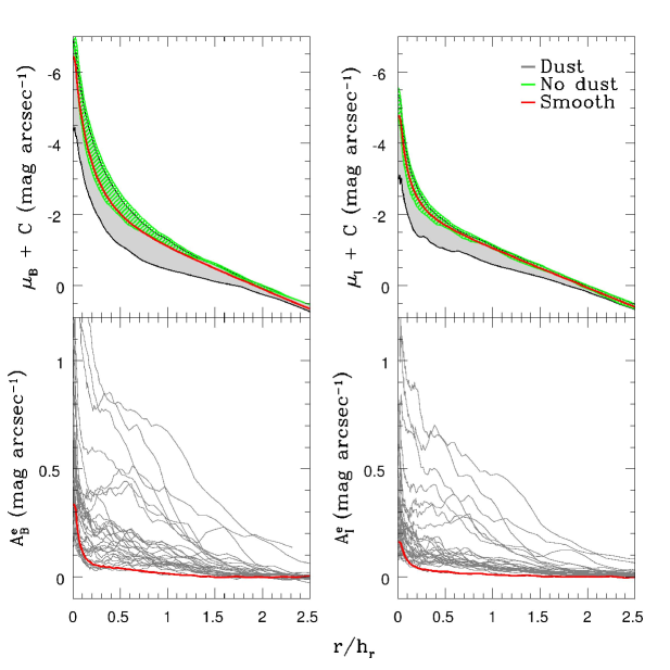
Figure 13.— Face-on surface brightness and attenuation profiles of the 30 best fitting clumpy-dust models with spiral structure, in the B (left) and I (right) bands. Upper panels show the range of model surface brightness profiles with dust (gray full shaded region) and without dust (green dashed shaded region). The red line indicates the profile for our fiducial model with a smooth dust and light distribution (see text). Lower panels show the residuals between the profiles of models with and without dust, i.e., an azimuthally averaged attenuation profile.

5.3. Face-on surface brightness and color profiles

While the attenuation maps presented show where the attenuation occurs, and we can quantify the filling factor of this attenuation, neither tell us directly the light-weighted attenuation as a function of radius, i.e. what fraction of the total light in a given annulus is attenuated. Therefore we construct surface brightness profiles both with and without dust for our best fitting models, as well as the smooth model from Popescu et al. (2000). We plot these surface brightness profiles and the difference between the models with and without dust in Figure 13. The residual between models with and without dust ($\mu-\mu_{\rho_{d}=0}$, where $\mu$ and $\mu_{\rho_{d}=0}$ denote the surface brightness in the B or I bands for models with and without dust, respectively), is a measure of the azimuthally-averaged attenuation as a function of radius. We find that most models have very low attenuation at all radii, with 90% of the models having $A_{B,I}^{e}=\mu_{B,I}-\mu_{B,I,\rho_{d}=0}\leq 0.1$ mag at $r/h_{r}=1.5$. Average $A_{\lambda}^{\rm e}$ values at 0.5, 1, and 2 $h_{r}$ are 0.20, 0.12, and 0.03 mag in the B band and 0.12, 0.08, and 0.04 mag in the I band. In general, the clumpy dust models have both higher attenuation and more variability at all radii than the fiducial model with a smooth dust distribution and no spiral structure. Additionally, the models with more attenuation also appear to have type-II (Freeman, 1970) surface brightness profiles. The low amounts of face-on attenuation imply that measured kinematics of face-on galaxies are minimally affected by dust attenuation (Bershady et al., 2010b).

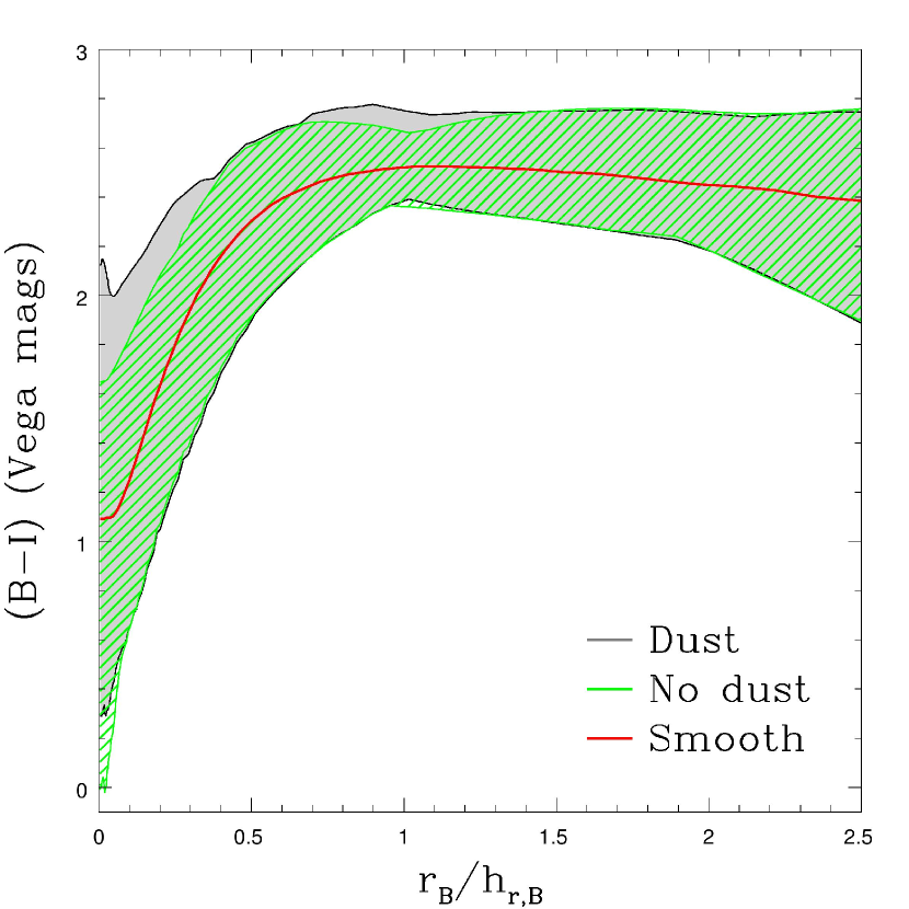
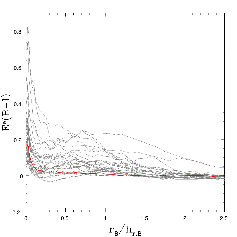
Figure 14.— Color profiles and reddening: (a) Radial B-I color profiles of the clumpy-dust models, with and without dust, and the fiducial model illustrated in Figure 13 with the same legend. (b) Effective color-excess profile in B-I.

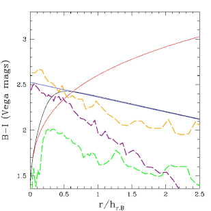
Figure 15.— Color profile contributions without dust for the fiducial model with smooth dust and no spiral structure, from Figure 13, compared to observed color profiles for low-inclination spiral galaxies. Model bulge and disk color profiles are shown by the red and blue solid lines, respectively. The total model color profile is in black. Three observed galaxy color profiles from de Jong (1996a) are overlaid with dashed lines: UGC 7450 (green), UGC 2064 (orange), and UGC 11628 (purple). These examples are discussed in the text.

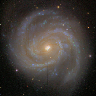
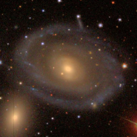
Figure 16.— Images of the three low-inclination galaxies with color profiles shown in Figure 15: UGC 7450 (left; SDSS color composite, 400 arcsec field of view), UGC 2064 (middle; V band image from de Jong 1996b, 100 arcsec field of view) and UGC 11628 (right; SDSS color composite, 200 arcsec field of view).

Radial profiles of $B-I$ color and the attenuation color excess $E^{\rm e}(B-I)=(B-I)-(B-I)_{\rho_{d}=0}$ are plotted in Figure 14. The inner region is unusually blue, with a strong gradient toward bluer central colors. Recall that we have simply adopted the bulge parameters from the literature for smooth-dust models of NGC 891. The global (disk + bulge) color profile rapidly reddens with increasing radius until $\sim$1 disk scale-length, at a rate of roughly $\sim 3(r/h_{r})$ mag in $B-I$ for $r/h_{r}<0.5$. At larger radii, all but two models then have color profiles which become monotonically bluer with increasing radius at a modest rate of $\sim 0.1(r/h_{r})$ mag, where we expect the light from the disk dominates. However, the $B-I$ color remains quite red ($>2$ mag) even at large radii, while $E^{\rm e}(B-I)$ remains very small given the small values for the attenuation seen in Figure 13. A few ($\sim$5) profiles with dust become bluer than their dust-free counterparts at radii $<$ 1 B band scale-length, due to scattering.

5.4. Low-inclination Counterparts

Since a blue bulge and red disk are not commonly found in face-on spiral galaxy samples, it is worth exploring whether these results found both from smooth and clumpy dust models are an artifact of inaccuracies of the modeling and radiative transfer or an insight into unusual properties of this extragalactic system viewed edge-on. First, as the left panel of Figure 13 shows, both the smooth-dust model from the literature for NGC 891’s disk and our clumpy-dust models produce comparable colors (bulge colors are the same by construction). Hence at least the outer portion of these color profiles are not due solely to adding clumpiness and spirality to the models.

To further investigate this issue we plot the color contributions of the bulge and the disk independently for the fiducial model with zero dust in Figure 15. As we anticipated, the blue central color is entirely due to the bulge, while the disk, with a central $B-I$ color a little redder than 2.5 mag, starts dominating the color profile at $r>0.5h_{r}$. For a bulge as red as an early-type stellar system (e.g., gm spectral-type; Bershady 1995) we might expect $B-I\sim 2.3$ mag. In contrast, for a typical disk we might expect $B-I$ between 1.5 and 2 mag (de Jong, 1996a). However, galaxies of a given morphological type have a large scatter around any mean color values. As examples, we overlay color profiles from de Jong (1996a) in Figure 15 for UGC 7450, UGC 2064, and UGC 11628. These are three low-inclination systems of type SABab/SABbc, not unlike the putative morphological type of NGC 891 classified from an edge-on view. Images of these systems are shown in Figure 16.

UGC 2064 and UGC 11628 both have red disks consistent with that of NGC 891, at least in the inner regions. The disk of UGC 2064, however has comparable color to that of the model for NGC 891 out to well beyond $2h_{r}$, while UGC 11628 has enhanced star-formation at large radii. Both appear to have sufficiently strong spiral structure at larger radii to explain the asymmetry in star-formation indicators seen in NGC 891, if these systems were viewed edge-on. In contrast to the central colors of these galaxies, UGC 7450’s central color profile is much bluer than the disk, and is consistent with the model for NGC 891. The reason UGC 7450’s central light profile is so blue is because there exists a modest, nuclear ring of star formation, visible in Figure 16). While this feature is not a bulge per se, it could be mimicked by a bulge component with a strong inner gradient, as seen in the smooth model of NGC 891. While the unusual color profile in the models are therefore possible, it is impossible to discount the (perhaps likely) possibility that it is due simply to the inability of optical images to probe the dust-obscured inner part of the galaxy.

5.5. Inclination corrections to integrated magnitudes

5.5.1 The Tully-Fisher Relation

The attenuation of a disk galaxy is dependent on that galaxy’s inclination in addition to the detailed geometry of the dust (see Witt et al. 1992 for a forceful discussion of this issue). When computing a disk galaxy’s integrated luminosity for, e.g. TF studies, this attenuation must be corrected for. Multiple approaches to computing the attenuation as a function of inclination exist in the literature. Tully & Fouque (1985) constructed an attenuation correction based on theoretical formalism assuming a smooth dust slab mixed homogeneously with the stars in the slab, with a fraction of starlight above and below the slab. This model can be parameterized as

$$A_{\lambda}^{i} =-2.5\times\log$$

$$\left[f(1+e^{-\tau_{\lambda}\sec i})+(1-2f)\left(\frac{1-e^{-\tau_{\lambda}\sec i}}{\tau_{\lambda}\sec i}\right)\right],$$ (14)

where $f$ is the fraction of light outside the slab of dust and $\tau_{\lambda}$ is the optical depth. Giovanelli et al. (1994) created an empirical formalism for the attenuation correction, parametrized by the inclination-corrected HI line-width W${}_{R,I}^{i}$ (Tully et al., 1998), and given by

$$A_{\lambda}^{i}=A_{\lambda}^{i=0}-(\alpha_{\lambda}+\beta_{\lambda}(\log W_{R,I}^{i}-2.5))\log\left(\frac{a}{b}\right)$$ (15)

and

$$\frac{b}{a}=\sqrt{\cos^{2}(i)\,(1-q^{2})+q^{2}}.$$ (16)

Here $A_{\lambda}^{i=0}$ is the face-on attenuation, $(a/b)$ is the axis ratio, $\alpha_{\lambda}$ and $\beta_{\lambda}$ are constants that depend on the bandpass, and q is the intrinsic axial ratio. Both functions are optimized to minimize scatter in the observed TF relation.

To investigate the inclination-dependence of the attenuation on integrated magnitudes for NGC 891-like galaxies, we photometered all of our 30 best-fitting clumpy-dust models rendered at a range of inclinations, with and without dust. As before, the flux ratio between a model with and without dust allows us to compute the attenuation. We perform the same analysis for our fiducial smooth model.

We plot the inclination-dependent attenuation in both HST bands in Figure 17. The clumpy models have statistically higher attenuation at lower inclinations than the smooth model, while at high inclinations they are comparable. This indicates that fitting smooth radiative transfer models to edge-on galaxies statistically underestimates the true amount of face-on extinction by an average of 0.1 and 0.06 mag and a maximum of 0.45 and 0.32 mag in B and I bands, respectively.

We have also fit both the empirical Giovanelli et al. (1994) and theoretical (slab-model) Tully & Fouque (1985) attenuation functions to the clumpy models. Essentially this is equivalent to a calibration (in a least-squares fitting sense) of the functional parameters of these formalisms to our RT models. The fitting is done only for inclinations $<$80^∘, since the theoretical function is discontinuous and the empirical function is strongly dependent on the axial ratio at purely edge-on inclinations. While both functions do a credible job of fitting the models at inclinations between 0 and 80^∘, neither adequately predict the increase in attenuation at inclinations $>$80^∘. This is not particularly worrisome for TF studies; such high inclinations are dis-favored on the prejudicial suspicion that indeed attenuation-corrections based on these formalisms in this inclination regime are problematic.

However, what is relevant for TF studies are the differences between the attenuation values used in the literature (dotted lines in Figure 17), and the values we find using the same formalisms calibrated to our radiative transfer models of NGC 891 (solid lines). It is also astrophysically interesting to note how the functional parameters change. For example, we find that in both bands the theoretical formalism based on the simple slab model used in the literature differs from that calibrated against our clumpy models almost entirely in the choice of the face-on attenuation: The fraction of light above and below the dust slab, $f$, is almost unchanged between the fit to the clumpy models and that used in Verheijen (2001). In contrast, the face-on attenuation is roughly doubled in the literature for both the B and I bands, from our fit value of 0.33 to 0.81 in Verheijen (2001) for $\tau_{B}$ and from 0.17 to 0.28 for $\tau_{I}$.

For the empirical formalism we also plot in Figure 17 the attenuation function for literature parameters of $\alpha_{\lambda}$ and $\beta_{\lambda}$ from Verheijen & Sancisi 2001 ($\alpha_{B}=1.57$, $\alpha_{I}=0.92$, $\beta_{B}=2.75$, and $\beta_{I}=1.63$) and a value of W${}_{R,I}^{i}$ appropriate for the observed rotation curve of NGC 891; and also the attenuation function calibrated to our clumpy models, fixing $\alpha_{\lambda}$ and $\beta_{\lambda}$ at the literature values but allowing W${}_{R,I}^{i}$ to vary. For both inclination corrections we follow Giovanelli et al. 1994 and convert between $i$ and $(a/b)$ using $q=0.13$. For the empirical fit using literature parameters we adopt $W_{R,I}^{i}=424$ km s^-1, twice the value for the maximum gas velocity in NGC 891 given by hyperLEDA (Paturel et al., 2003). In contrast, our best calibration of this formalism requires $W_{R,I}^{i}=189\pm 25$ km s^-1 and $202\pm 34$ km s^-1 in the B and I bands, respectively. This value for $W_{R,I}^{i}$ is less than half of what is expected for NGC 891 based on the observed H I gas velocity but consistent between the two bands within the uncertainties. In this formalism allowing $W_{R,I}^{i}$ to vary is equivalent to varying $\alpha_{\lambda}$ while holding $W_{R,I}^{i}$ and $\beta_{\lambda}$ constant, and we find that for $W_{R,I}^{i}=424$ km s^-1 our clumpy models predict $\alpha_{B}=0.61$ and $\alpha_{I}=0.40$, significantly lower than values from the literature.

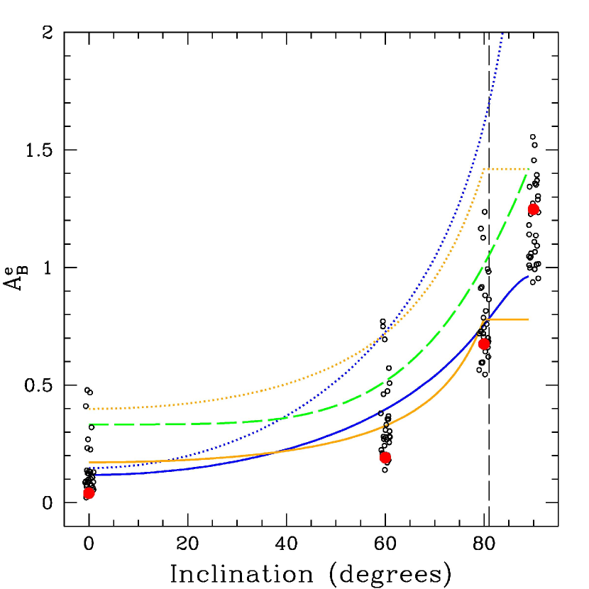
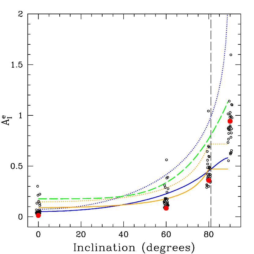
Figure 17.— Inclination-dependent attenuation in B (left) and I (right) bands. Black open circles are clumpy models and the red dots are the smooth model. Horizontal scatter in the black open circles is random noise added to increase the visibility of overlapping data points. Orange lines denote model predictions using the Tully & Fouque (1985) formalism, while blue lines use the Giovanelli et al. (1994) formalism as given in Verheijen (2001). Solid lines represent fits of these analytic formalisms to the clumpy models between 0$\leq$i$\leq$80 degrees; dotted lines represent these analytic formalisms for parameters in the literature (e.g., Verheijen (2001)), relevant for NGC 891 (see text). The green dashed line shows the results for NGC 891 using a model that does not include spirality but has a star-forming thin disk (Tuffs et al., 2004; Driver et al., 2008).

In both cases our results imply significant revision downward for dust-corrections in TF studies. In the $B$ band for NGC 891-like galaxies observed at $i=60^{\circ}$ this is equivalent to a $\sim$60% decrease in the mass-to-light ratio, and intrinsic $B-I$ colors which are $\sim$30% bluer. More fundamentally, our results imply that the implicit assumption in the literature, namely that the TF-scatter can be minimized as a metric for constraining other astrophysical quantities, may be incorrect in general. Certainly this assumption appears to fail in the case of determining the attenuation for galaxies like NGC 891.

5.5.2 Co-moving Star-formation Rates and Stellar Mass Density

Many estimates in the literature of star-formation rates and stellar mass density in cosmological volumes are based on counting the number of UV through near-infrared photons emitted from galaxies (see Driver et al. 2008 for a recent summary). It is well known that these estimates are subject to uncertainties in the attenuation, which, as we have seen, are inclination dependent. Because most star-formation appears to take place in a thin, dusty disk layer, the details of radiative transfer and the impact of a clumpy dust distribution are likely to be particularly important in predicting the emergent flux and its SED. In the context of matching optical and far-infrared and sub-millimeter observations to obtains bolometric estimates of star-formation rates, Driver et al. (2008) have explored the impact of embedding a thin, UV-bright disk into disk+bulge systems like the ones we have modeled here for NGC 891. Given this recent development, it is relevant to compare them to the models we have created here.

In Figure 17 we overplot a combined disk+bulge attenuation function derived for a smooth, axisymmetric RT model of NGC 891 from Tuffs et al. (2004) (green dashed lines). This model features a thin, UV-bright disk in addition to the bulge, thick disk, and dust disk components. While all the disk components are represented by smooth double-exponentials, the effects of clumpy star formation in the thin disk are approximated by artificially reserving a fraction of the input UV luminosity to be re-emitted by the dust grains. Spiral arms are not included in either the dust or light components. The general form of the inclination dependence comes from Driver et al. (2008), while the prescription for combining the bulge and disk attenuation into a total attenuation for NGC 891 follows the method and data given in Tuffs et al. (2004).

This model does a much better job than either the Verheijen (2001) or Giovanelli et al. (1994) parameterizations, and shows that the addition of a star-forming, thin disk is roughly equivalent to adding clumpy dust in spiral arms for our models with higher attenuation. This likely implies that modeling either just a thin disk or spiral arms and clumpy dust is not enough to constrain the total attenuation.

We can robustly conclude that, for galaxies with dust distributions like NGC 891, previous estimates of attenuation corrections to smooth stellar light distribution were too large. While it is tempting to infer that therefore so too were the resulting estimates for star-formation rates previously over-estimated, this inference requires a better understanding of the contribution of star-light that is not smoothly distributed. It would not be surprising that in order to truly determine the attenuation of spiral disks both the detailed structure of star-forming regions and spirality must be considered simultaneously.

5.6. Inclination dependence to the attenuation curve

In Section 5.2 we considered the values of the attenuation curve parameter R_B,B-I at several different radii. Here, we consider the value that applies for the integrated light of a galaxy as a function of inclination. Using the same definition of the attenuation curve parameter R_B,B-I as before, in Figure 18 we plot R_B,B-I histograms for our 30 best fitting models at the four inclinations of Figure 17. We also include the values for R_B,B-I of the smooth model as well as literature values for a foreground screen (Cardelli et al., 1989) and star-forming galaxies (Calzetti et al., 2000). We first note the dependence of R_B,B-I with inclination, with the peak of the R_B,B-I histogram increasing by $\sim$0.75 between i=0^∘ and 80^∘. This dependence is due to a combination of scattering and projection effects, as well as the saturation of the color excess $E(B-I)$ at higher values of $A_{B}$ (Matthews & Wood, 2001). The smooth model shows this trend as well, although it has a slightly lower R_B,B-I value at all non-edge-on inclinations.

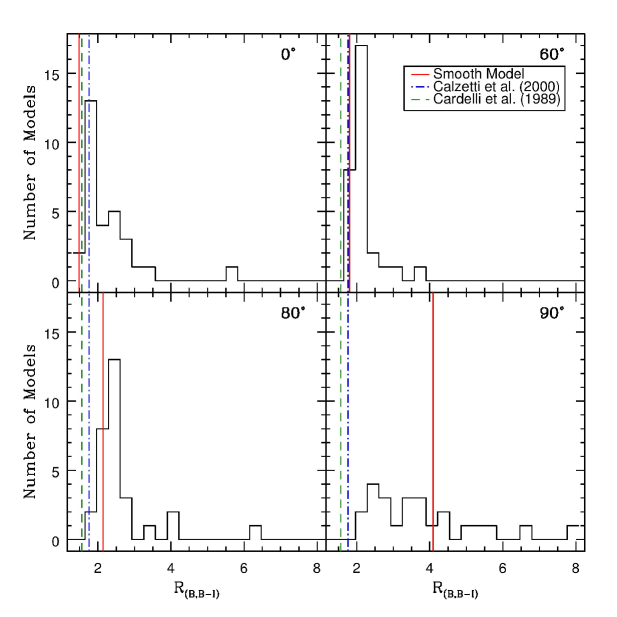
Figure 18.— R_B,B-I distribution for our 30 best-fitting clumpy models at i=0, 60, 80, and 90^∘. The smooth model is shown as a red line. The galactic foreground screen model of Cardelli et al. (1989) is plotted as a green dashed line. The star forming galaxy model of Calzetti et al. (2000) is plotted as the blue dot-dash line.

At edge-on inclination R_B,B-I is much more variable between our models. This is due mainly to geometrical projection effects (from having large amounts of relatively unattenuated flux above and below the midplane) which cause the color excess to become very small for some ($\sim$5) models. For these models R_B,B-I becomes very large. Rather than dilute the meaning of the figure we choose not to plot these models. Even excluding the models with the largest values of R_B,B-I, there is a much larger dispersion in the attenuation curve parameter at edge-on inclination, with a general preference toward larger values of R_B,B-I. This is true even for the smooth model, which at lower inclinations has a lower-than-average R_B,B-I but at 90^∘ has a grayer attenuation curve than most of the non-axisymmetric models.

The peak of the R_B,B-I histogram occurs at larger values than the foreground screen at all inclinations, from a difference of $\sim$0.25 at face-on inclinations to $\sim$1 at 80^∘. This means that for a given attenuation the internal reddening is grayer (i.e. less wavelength-dependent) than expected for a simple screen. We find good agreement between the Calzetti et al. (2000) attenuation model and our simulations at face-on inclinations, but at larger inclinations our RT models have systematically larger values of R_B,B-I. This difference is likely due to selection effects in the empirical estimates, both because there are more galaxies with inclinations $<60^{\circ}$ than there are with i $>80^{\circ}$, and the Calzetti et al. (2000) sample is selected based partly on high UV emission which is most likely to be from galaxies at or near face-on orientation. At edge-on inclinations the attenuation curve has a low dependence on color, but the grayness of the curve is highly model-dependent.

6. Conclusion

We have optimized a 3D Monte Carlo scattered light RT model to HST F450W and F814W images (essentially B and I band) of NGC 891. Our model is the first RT model involving realistic dust clumping and spirality to be quantitatively fit to imaging data. Dust is treated using a fractal algorithm, while spirality is included using a logarithmic spiral parameterization with a coarsely adjustable arm-interarm width ratio.

In order to enhance the effects of non-axisymmetric dust we constructed $\Delta A_{\lambda}^{\rm e}$ maps using smooth models from the literature, then used the coefficients of a high-order shapelet image reconstruction to compare our clumpy models with the data. Computing Monte Carlo models at a high resolution is computationally expensive, so we used a genetic algorithm to find ’good’ solutions in our many-dimensional parameter space in a reasonable amount of time. The efficiency of the genetic algorithm also allowed us to include a wide range of parameter values in order to fully probe our parameter space.

We computed $30\times 50$-generation runs of the genetic algorithm and find a fairly wide variety of parameter values in the best-fitting models. Some of this variety is likely due to complex interdependencies of the free parameters, (e.g. central disk surface brightness, scale length, and scale height for dust and stars), while the rest is the result of degeneracies from choosing such a large parameter space.

Despite these degeneracies, the best-fitting models from our 30 genetic algorithm runs do a credible job at mimicking the general features of the edge on profile of NGC 891. Perhaps more importantly, our models appear to be realistic simulations of face-on galaxies as well. While some of this is due to our more advanced treatment of spirality, which automatically creates more realistic-looking spiral features than previous work, it is important to note that the amount of spirality and clumping were free parameters; in 29 out of 30 runs our algorithm chose minima with clear spirality (despite not constraining the direction of the spiral structure) and the median fraction of dust placed in clumps is 58%. This is the first quantitative measurement of the clumpiness of dust in edge-on spiral galaxies that is not dependent on empirically matching IR SEDs but rather on observable dust morphology, and is in general agreement with clumpy fractions obtained through the SED fitting method.

The preference for visible spiral features and clumpy dust has significant implications for the face-on attenuation in spiral galaxies. We find that while overall our models prefer low (A_B and $A_{I}<1$) face-on attenuation, clumping and spirality produce localized regions of enhanced dust absorption, creating Type II surface brightness profiles as well as very small ($\lesssim 10\%$) high attenuation filling factors. These clumps result in larger total attenuation than a smooth model at low inclinations while having comparable attenuation when viewed edge-on, where the clumps overlap to more closely mimic a smooth dust distribution.

Additionally, we probed the effect of the dust when viewed as a foreground screen on background light sources. While still highly concentrated in spiral arms, we find significantly higher optical depths than would be suspected when only considering the attenuation — on average 1.2 mag larger in the B band and 0.5 mag larger in the I band at one scale-length. The discrepancy between the optical depths and the attenuation comes from both the admixture of dust and starlight as well as the effect of scattering. The optical depths of our models are broadly in agreement with some measurements from the literature but not others, which may be a result of a large range in the optical depths in real galaxies.

We find that our models predict a blue bulge and red disk for NGC 891 when viewed face-on, regardless of the attenuation. The smooth, axisymmetric fiducial model from the literature which we use to construct our $\Delta A_{\lambda}^{\rm e}$ maps also has this unusual morphology, and while we use bulge parameters from the the literature the red disk is present in our models even though we allowed the central disk emissivities and scale-lengths and heights to vary. While perhaps not common, an inspection of surface brightness profiles of a sample of face-on galaxies shows that blue, star-forming cores and red disks do exist in intermediate-type spirals. However, we observe neither of these features in the Milky Way, despite the frequently claimed similarity between NGC 891 and our own galaxy.

Even with the increased face-on attenuation in the clumpy models relative to smooth dust models, virtually all of our simulations have smaller attenuations at all inclinations than would be expected given corrections based on simple radiative transfer models and empirical formulae in common use in the literature. This result indicates that TF studies need reduced attenuation corrections by typically 0.5 mag in B band at i=60^∘, and 0.25 mag in I at the same inclination. Inclination corrections based on more advanced RT models of edge-on spiral galaxies, however, do fit some of our dustier simulations very well and point to the need to include star-forming regions as well as spirality in future efforts.

Our models also predict a significantly grayer attenuation curve than found for both a simple foreground screen of dust and an attenuation curve derived from UV-bright star forming galaxies. We also find that the attenuation curve becomes $\sim$40% grayer with inclination, something not considered in currently favored attenuation models. Both the large amount of edge-on variability of the models and the gradual systematic increase in R_B,B-I with inclination are a strong caution for extrapolating empirically determined attenuation curves to objects with high inclinations.

We have not been able to produce clumpy dust models with the realistic high-latitude dust “chimneys” seen in the data, although it is unlikely including them would significantly change our results due to their low spatial frequency and small size. It is unclear whether the lack of high-latitude dust in our models is due to a poor choice of fitness function or the fractal geometry, although the fractal algorithm is certainly not optimized to produce extended dust “fingers”. We find that the shapelet coefficients of the data have fewer extreme (large or small) coefficient values as well as a better balance of power between odd and even coefficients than most of the clumpy models; these observations will help us to improve our fitness metric.

Finding a method for computing model fitnesses more sensitive to small-scale structures would help improve the reproduction of dust substructure regardless of the clumping formalism. Multi-stage fitting processes may be useful to reduce the size of parameter space; global parameters (like central brightness, scale-length, and spirality) could be determined from smooth, lower resolution models covering the whole galaxy then fed into a much higher resolution model where the only free parameters relate to the dust density and clumping.

In producing quantitative RT modeling which includes spirality and clumping we have made the first foray into a new generation of highly detailed simulations that produce images capable of resembling real galaxy morphologies at any inclination. Extending clumpy, non-axisymmetric models based on our prototype to larger fields of view and large wavelength baselines, we expect to be able to constrain the 3D structure of spiral disks using physically realistic simulations as well as more accurately predict thermal dust re-emission in the mid-infrared. Additionally, the increase in resolution of far-IR images provided by the Herschel Space Observatory will enable the next generation of SED models to fit SEDs to multiple positions of individual galaxies, where the signatures of non-axisymmetric structures will be more difficult to average out. By creating a realistic form of spiral structure and dust clumping we provide a blueprint for future work in this area.

References

- Baes et al. (2003) Baes, M., et al. 2003, MNRAS, 343, 1081
- Baes et al. (2011) Baes, M., Verstappen, J., De Looze, I., et al. 2011, ApJS, 196, 22
- Bahcall (1983) Bahcall, J. N. 1983, ApJ, 267, 52
- Bershady (1995) Bershady, M. A. 1995, AJ, 109, 87
- Bershady et al. (2010a) Bershady, M. A., Verheijen, M. A. W., Swaters, R. A., Andersen, D. R., Westfall, K. B., & Martinsson, T. 2010, ApJ, 716, 198
- Bershady et al. (2010b) Bershady, M. A., Verheijen, M. A. W., Westfall, K. B., Andersen, D. R., Swaters, R. A., & Martinsson, T. 2010, ApJ, 716, 234
- Bianchi (2008) Bianchi, S. 2008, A&A, 490, 461
- Bianchi et al. (1996) Bianchi, S., Ferrara, A., & Giovanardi, C. 1996, ApJ, 465, 127
- Bianchi & Xilouris (2011) Bianchi, S., & Xilouris, E. M. 2011, A&A, 531, L11
- Bosch (2010) Bosch, J. 2010, AJ, 140, 870
- Calzetti et al. (2000) Calzetti, D., Armus, L., Bohlin, R. C., Kinney, A. L., Koornneef, J., & Storchi-Bergmann, T. 2000, ApJ, 533, 682
- Calzetti et al. (1994) Calzetti, D., Kinney, A. L., & Storchi-Bergmann, T. 1994, ApJ, 429, 582
- Cardelli et al. (1989) Cardelli, J. A., Clayton, G. C., & Mathis, J. S. 1989, ApJ, 345, 245
- Dalcanton et al. (2004) Dalcanton, J. J., Yoachim, P., & Bernstein, R. A. 2004, ApJ, 608, 189
- de Jong (1996a) de Jong, R. S. 1996, A&A, 313, 377
- de Jong (1996b) de Jong, R. S. 1996, Journal of Astronomical Data, 2, 1
- Domingue et al. (2000) Domingue, D. L., Keel, W. C., & White, R. E., III 2000, ApJ, 545, 171
- Draine (2003) Draine, B. T. 2003, ApJ, 598, 1017
- Driver et al. (2008) Driver, S. P., Popescu, C. C., Tuffs, R. J., Graham, A. W., Liske, J., & Baldry, I. 2008, ApJ, 678, L101
- Elmegreen (1997) Elmegreen, B. G. 1997, ApJ, 477, 196
- Elmegreen & Elmegreen (1982) Elmegreen, D. M., & Elmegreen, B. G. 1982, MNRAS, 201, 1021
- Elmegreen & Falgarone (1996) Elmegreen, B. G., & Falgarone, E. 1996, ApJ, 471, 816
- Freeman (1970) Freeman, K. C. 1970, ApJ, 160, 811
- Garcia-Burillo et al. (1992) Garcia-Burillo, S., Guelin, M., Cernicharo, J., & Dahlem, M. 1992, A&A, 266, 21
- Garcia-Burillo & Guelin (1995) Garcia-Burillo, S., & Guelin, M. 1995, A&A, 299, 657
- Gerard (1973) Gerard, E. 1973, A&A, 28, 95
- Giovanelli et al. (1994) Giovanelli, R., Haynes, M. P., Salzer, J. J., Wegner, G., da Costa, L. N., & Freudling, W. 1994, AJ, 107, 2036
- Gordon et al. (1997) Gordon, K. D., Calzetti, D., & Witt, A. N. 1997, ApJ, 487, 625
- Holwerda et al. (2005) Holwerda, B. W., Gonzalez, R. A., Allen, R. J., & van der Kruit, P. C. 2005, AJ, 129, 1396
- Holwerda et al. (2009) Holwerda, B. W., Keel, W. C., Williams, B., Dalcanton, J. J., & de Jong, R. S. 2009, AJ, 137, 3000
- Howk & Savage (1997) Howk, J. C., & Savage, B. D. 1997, AJ, 114, 2463
- Howk & Savage (1999) Howk, J. C. & Savage, B. D. 1999, AJ, 117, 2077
- Howley et al. (2008) Howley, K. M., Geha, M., Guhathakurta, P., Montgomery, R. M., Laughlin, G., & Johnston, K. V. 2008, ApJ, 683, 722
- Indebetouw et al. (2006) Indebetouw, R., Whitney, B. A., Johnson, K. E., & Wood, K. 2006, ApJ, 636, 362
- Joung & Mac Low (2006) Joung, M. K. R., & Mac Low, M.-M. 2006, ApJ, 653, 1266
- Kamphuis et al. (2007) Kamphuis, P., Holwerda, B. W., Allen, R. J., Peletier, R. F., & van der Kruit, P. C. 2007, A&A, 471, L1
- Kelly & McKay (2004) Kelly, B. C., & McKay, T. A. 2004, AJ, 127, 625
- Kennicutt (1981) Kennicutt, R. C., Jr. 1981, AJ, 86, 1847
- Keppel et al. (1991) Keppel, J. W., Dettmar, R.-J., Gallagher, J. S., III, & Roberts, M. S. 1991, ApJ, 374, 507
- Kuchinski et al. (1998) Kuchinski, L. E., Terndrup, D. M., Gordon, K. D., & Witt, A. N. 1998, AJ, 115, 1438
- Kuijken (2006) Kuijken, K. 2006, A&A, 456, 827
- Kylafis & Bahcall (1987) Kylafis, N. D., & Bahcall, J. N. 1987, ApJ, 317, 637
- Lewis et al. (2009) Lewis, N. K., Cook, T. A., Wilton, K. P., et al. 2009, ApJ, 706, 306
- Mapelli et al. (2008) Mapelli, M., Moore, B., & Bland-Hawthorn, J. 2008, MNRAS, 388, 697
- Massey et al. (2004) Massey, R., Refregier, A., Conselice, C. J., David, J., & Bacon, J. 2004, MNRAS, 348, 214
- Mathis et al. (1977) Mathis, J. S., Rumpl, W., & Nordsieck, K. H. 1977, ApJ, 217, 425
- Mathis et al. (2002) Mathis, J. S., Whitney, B. A., & Wood, K. 2002, ApJ, 574, 812
- Matthews & Wood (2001) Matthews, L. D., & Wood, K. 2001, ApJ, 548, 150
- Mihos et al. (1999) Mihos, J. C., Spaans, M., & McGaugh, S. S. 1999, ApJ, 515, 89
- Misiriotis et al. (2000) Misiriotis, A., Kylafis, N. D., Papamastorakis, J., & Xilouris, E. M. 2000, A&A, 353, 117
- Misiriotis & Bianchi (2002) Misiriotis, A., & Bianchi, S. 2002, A&A, 384, 866
- Oosterloo et al. (2007) Oosterloo, T., Fraternali, F., & Sancisi, R. 2007, AJ, 134, 1019
- Paturel et al. (2003) Paturel G., Petit C., Prugniel P., Theureau G., Rousseau J., Brouty M., Dubois P., Cambrésy L., 2003, A&A, 412, 45
- Perrin et al. (1995) Perrin, J.-M., Darbon, S., & Sivan, J.-P. 1995, A&A, 304, L21
- Pierini et al. (2002) Pierini, D., Majeed, A., Boroson, T. A., & Witt, A. N. 2002, ApJ, 569, 184
- Pierini et al. (2004) Pierini, D., Gordon, K. D., Witt, A. N., & Madsen, G. J. 2004, ApJ, 617, 1022
- Popescu et al. (2000) Popescu, C. C., Misiriotis, A., Kylafis, N. D., Tuffs, R. J., & Fischera, J. 2000, A&A, 362, 138
- Popescu et al. (2011) Popescu, C. C., Tuffs, R. J., Dopita, M. A., et al. 2011, A&A, 527, A109
- Rand et al. (1990) Rand, R. J., Kulkarni, S. R., & Hester, J. J. 1990, ApJ, 352, L1
- Refregier (2003) Refregier, A. 2003, MNRAS, 338, 35
- Sankrit & Wood (2001) Sankrit, R., & Wood, K. 2001, ApJ, 555, 532
- Schweizer (1976) Schweizer, F. 1976, ApJS, 31, 313
- Sirianni et al. (2005) Sirianni, M., et al. 2005, PASP, 117, 1049
- Strong (1978) Strong, A. W. 1978, A&A, 66, 205
- Swaters et al. (1997) Swaters, R. A., Sancisi, R., & van der Hulst, J. M. 1997, ApJ, 491, 140
- Tuffs et al. (2004) Tuffs, R. J., Popescu, C. C., Völk, H. J., Kylafis, N. D., & Dopita, M. A. 2004, A&A, 419, 821
- Tully & Fouque (1985) Tully, R. B., & Fouque, P. 1985, ApJS, 58, 67
- Tully et al. (1998) Tully, R. B., Pierce, M. J., Huang, J.-S., Saunders, W., Verheijen, M. A. W., & Witchalls, P. L. 1998, AJ, 115, 2264
- van der Kruit (1984) van der Kruit, P. C. 1984, A&A, 140, 470
- Verheijen (2001) Verheijen, M. A. W. 2001, ApJ, 563, 694
- Verheijen & Sancisi (2001) Verheijen, M. A. W., & Sancisi, R. 2001, A&A, 370, 765
- White (1979) White, R. L. 1979, ApJ, 229, 954
- White et al. (2000) White, R. E., III, Keel, W. C., & Conselice, C. J. 2000, ApJ, 542, 761
- Witt (1977) Witt, A. N. 1977, ApJS, 35, 1
- Witt et al. (1992) Witt, A. N., Thronson, H. A., Jr., & Capuano, J. M., Jr. 1992, ApJ, 393, 611
- Witt & Gordon (1996) Witt, A. N., & Gordon, K. D. 1996, ApJ, 463, 681
- Witt & Gordon (2000) Witt, A. N., & Gordon, K. D. 2000, ApJ, 528, 799
- Wood et al. (1996) Wood, K., Bjorkman, J. E., Whitney, B. A., & Code, A. D. 1996, ApJ, 461, 828
- Wood & Jones (1997) Wood, K., & Jones, T. J. 1997, AJ, 114, 1405
- Wood & Reynolds (1999) Wood, K., & Reynolds, R. J. 1999, ApJ, 525, 799
- Wood et al. (1999) Wood, K., Crosas, M., & Ghez, A. 1999, ApJ, 516, 335
- Wood & Loeb (2000) Wood, K., & Loeb, A. 2000, ApJ, 545, 86
- Wood et al. (2005) Wood, K., Haffner, L. M., Reynolds, R. J., Mathis, J. S., & Madsen, G. 2005, ApJ, 633, 295
- Wood et al. (2010) Wood, K., Hill, A. S., Joung, M. R., Mac Low, M.-M., Benjamin, R. A., Haffner, L. M., Reynolds, R. J., & Madsen, G. J. 2010, ApJ, 721, 1397
- Xilouris et al. (1998) Xilouris, E. M., Alton, P. B., Davies, J. I., Kylafis, N. D., Papamastorakis, J., & Trewhella, M. 1998, A&A, 331, 894
- Xilouris et al. (1999) Xilouris, E. M., Byun, Y. I., Kylafis, N. D., Paleologou, E. V., & Papamastorakis, J. 1999, A&A, 344, 868
- Yusef-Zadeh et al. (1984) Yusef-Zadeh, F., Morris, M., & White, R. L. 1984, ApJ, 278, 186