Measurement Error Models in Astronomy

Abstract

I discuss the effects of measurement error on regression and density estimation. I review the statistical methods that have been developed to correct for measurement error that are most popular in astronomical data analysis, discussing their advantages and disadvantages. I describe functional models for accounting for measurement error in regression, with emphasis on the methods of moments approach and the modified loss function approach. I then describe structural models for accounting for measurement error in regression and density estimation, with emphasis on maximum-likelihood and Bayesian methods. As an example of a Bayesian application, I analyze an astronomical data set subject to large measurement errors and a non-linear dependence between the response and covariate. I conclude with some directions for future research.

1 Introduction

Measurement error is ubiquitous in astronomy. Astronomical data consists of passive observations of objects, whereby astronomers are able to directly measure the flux of an object as a function of wavelength, its location on the sky, and the time of the observation. Because the number of photons detected from an astronomical object follows a Poisson process, this makes the measurement of a source’s intensity intrinsically subject to measurement error, even if none is introduced from the detector. Therefore, the very nature of astronomical data makes measurement error unavoidable. Moreoever, quantities that are derived from an object’s observed emission, either by fitting a model to the spectral energy distribution (SED) or by employing scaling relationships, are also ‘measured’ (derived) with error. Examples include mass, metallicity, and distance. Often the measurement error on the derived quantities is significant. This is unfortunate as inference on the derived quantities is often the goal of astronomical data analysis. Therefore, there has been considerable interest in how to perform statistical inference in the presence of measurement error.

Measurement error is a problem that affects, at various levels, all scientific research. Because of this, numerous methods for handling measurement errors have been developed (Fuller 1987, Cheng & Van Ness 1999, and Carroll et al. 2006 are good references). In this contribution, I will present a survey of methods for handling measurement error that have been developed and used in astronomical data analysis. Because astronomical measurement errors are, in general, heteroskedastic (having different variances), I will limit my discussion to methods developed for heteroskedasticity. I will focus on situations where a deterministic relationship is not assumed between the variables, but where all variables of interest are random and are measured with error. Because of this, I will ignore situations where the measurement error is the only source of randomness in one’s data. An example of this type of situation is fitting a model to an observed spectrum, where the measurement error is the only source of randomness; i.e., in the absence of measurement error a deterministic relationship is assumed between, say, flux density and wavelength. Methods for handling measurement error in this case are relatively well-established, and typically one simply minimizes the usual $\chi^{2}$ statistic (e.g., Bevington 2003). However, it is worth pointing out that many complications may still exist, and more sophisticated methods may be needed, especially when dealing with low-count X-ray and $\gamma$-ray data (e.g., van Dyk et al. 2001) or when incorporating calibration unceratinties (Lee et al. 2011). Instead, I will focus on methods for analyzing data from astronomical samples, where the variables are a random sample from an underlying distribution. Within the context of regression, this implies that intrinsic scatter (referred to as equation error in the statistics literature) exists in the relationship among the variables, and thus a deterministic relationship is not assumed between the variables even without the presence of measurement error.

Most of the techniques I will discuss focus on accounting for measurement error in regression. The goal of regression is often to understand how one variable changes with another. For example, how does the mass of a black hole change as a function of the stellar velocity dispersion of the host galaxy’s bulge? Typically one simply estimates how the average value and dispersion of one variable depends on another. Measurement error statistical models are typically divided into two types: ‘functional’ and ‘structural’ models. In functional modeling, one assumes that the unknown true values of the variables are fixed, whereas in structural modeling the unknown true values of the variables have their own intrinsic distribution. As a result, in structural modeling one must parameterically model the distribution of the true values of the variables, whereas in functional modeling one does not. Density estimation is another important technique in astronomical data analysis, being the foundation for luminosity and mass function estimation. The methods I will discuss for handling measurement error in structural models are also applicable to density estimation, as in this case regression and density estimation are based on the same formalism. When discussing regression methods, I will refer to the ‘dependent’ variable as the response, and the ‘independent variables’ as the covariates.

2 Notation and Error Model

Throughout this work I will denote the measured response for the $i^{\rm th}$ data point as $y_{i}$, and the measured covariate for the $i^{\rm th}$ data point as $x_{i}$. I will denote the true values as $\eta_{i}$ and $\xi_{i}$, respectively. If there are $p>1$ covariates, then I will use the vectors $\vec{x_{i}}$ and $\vec{\xi_{i}}$. I will use $\vec{y}$ to denote the set of values of $y_{i}$ for each of the $n$ data points, $\vec{y}=[y_{1},\ldots,y_{n}]$. To denote the set of $x_{i}$, I will use $\vec{x}={x_{1},\ldots,x_{n}}$ if there is one covariate, and the $n\times p$ matrix $X=[\vec{x_{1}},\ldots,\vec{x_{n}}]$ if there are multiple covariates. I assume the classical additive error models throughout this review, unless otherwise specified:

$$\eta_{i} = f(\vec{\xi_{i}},\theta)+\epsilon_{i}$$ (1)

$$\vec{x_{i}} = \vec{\xi_{i}}+\vec{\epsilon_{x,i}}$$ (2)

$$y_{i} = \eta_{i}+\epsilon_{y,i}.$$ (3)

The function $f(\vec{\xi},\theta)$ describes how the mean value of $\eta$ depends on $\vec{\xi}$ as a function of the parameters, $\theta$. For example, for linear regression $f(\vec{\xi},\theta)=\alpha+\vec{\beta}^{T}\vec{\xi}$ with $\theta=(\alpha,\beta)$ denoting the slopes and intercept. The terms $\epsilon_{i},\vec{\epsilon_{x,i}},$ and $\epsilon_{y,i}$ are random variables denoting the intrinsic scatter in $\eta$ at fixed $\xi$ (i.e., the equation error), the measurement error in $\vec{x_{i}}$, and the measurement error in $y_{i}$, respectively. The random variables $\epsilon_{i},\vec{\epsilon_{x,i}},$ and $\epsilon_{y,i}$ are assumed to have zero mean and variances $Var(\epsilon_{i})=\sigma^{2},Var(\epsilon_{y,i})=\sigma^{2}_{y,i},$ and $Var(\vec{\epsilon_{x,i}})=\Sigma_{\vec{x},i}$. As is typical in astronomy, the parameter $\sigma^{2}$ is assumed to be unknown and a free parameter in the model, while the variances in the measurement errors, $\sigma^{2}_{y,i}$ and $\Sigma_{\vec{x},i}$, are assumed known. The measurement errors are assumed to be independent of $\epsilon_{i}$. In addition, for simplicity I also assume that the measurement errors in $y_{i}$ and $\vec{x_{i}}$ are independent, unless otherwise specified. However, this is not always true, and many methods are able to handle correlated measurement errors, see the references for individual techniques for further details.

Following Gelman et al. (2004), I will also typically use the notation $p(\cdot)$ to denote the probability density of the argument. For example, $p(x)$ denotes the marginal probability density of $x$, $p(y|x)$ denotes the conditional probability density of $y$ given $x$, and $p(y,x)$ denotes the joint probability density of $y$ and $x$. It should be understood that $p(\cdot)$ will not always have the same functional form, and that this must be inferred from context, i.e., it is not necessarily true that $p(x)=p(y)$ even if $x=y$. When this may be confusing, I use different symbols to denote different probability densities.

3 Effects of Measurement Error

Measurement error has the effect of blurring and broadening the distribution of quantities, similar to the blurring of astronomical images by a point spread function. This makes statistical inference based on the measured values biased, and smears out any trends in the data. The distribution of the measured quantities is obtained as

$$p(y,\vec{x})=\int\int p(y,\vec{x}|\eta,\vec{\xi})p(\eta,\vec{\xi})\ d\eta\ d\vec{\xi}.$$ (4)

Under the additive error model of § 2, Equation (4) simplifies to

$$p(y,\vec{x})=\int f(y-\eta)\int g(\vec{x}-\vec{\xi})p(\eta,\vec{\xi})\ d\vec{\xi}\ d\eta,$$ (5)

where $f(\cdot)$ and $g(\cdot)$ denote the probability distributions of the measurement errors $\epsilon_{y}$ and $\epsilon_{x}$, respectively. Equation (5) shows that under additive measurement error, the observed distribution of a set of quantities is the convolution of the intrinsic distribution with the measurement error distribution. Convolution has the effect of broadening distributions, which biases density estimation and masks trends.

Some of the effects of measurement error are illustrated in Figure 1. Here, I simulated a sample of covariates from a bimodal distribution, and simulated the response assuming a nonlinear relationship between $\eta$ and $\xi$. I then added large measurement error to both $\eta$ and $\xi$. As can be seen, measurement error has blurred out many of the features in the data set, and broadened the distributions.

Figure 1: Illustration of the effect of measurement error on regression and density estimation, using a simulated sample. The true distribution of the response and covariate (left), compared with the measured distribution (center). The error bars in the center plot denote the standard deviation of the Gaussian measurement errors. The measurement errors have effectively washed out any visual evidence for a tight non-linear relationship between the response and covariate. The right plot shows the distribution of the true and measured values of the covariate. The measurement errors have washed out any evidence for bimodality in the distribution, and significantly broadened it.

To further see how measurement error biases statistical inference for regression, consider the additive error model for linear regression, assuming one covariate. In addition, for simplicity assume that the measurement errors are homoskedastic (having the same variance) for both the response and covariate. If one were to ignore measurement error and proceed through the usual ordinary least-squares (OLS) analysis, then one would obtain the following estimates for the slope, variance in the intrinsic scatter, and uncertainty in the estimated slope (assume the intercept, $\alpha$, is known):

$$\hat{\beta}_{OLS} = \frac{Cov(x,y)}{Var(x)}=\frac{Cov(\xi,\eta)}{Var(\xi)+\sigma^{2}_{x}}$$ (6)

$$\hat{\sigma}^{2}_{OLS} = Var(y-\alpha-\hat{\beta}_{OLS}x)=(\beta^{2}-\hat{\beta}^{2}_{OLS})Var(\xi)+\hat{\beta}^{2}_{OLS}\sigma^{2}_{x}+\sigma^{2}_{y}+\sigma^{2}$$ (7)

$$Var(\hat{\beta}_{ols}) = \frac{\hat{\sigma}^{2}_{OLS}}{Var(x)}=\frac{\hat{\sigma}^{2}_{OLS}}{Var(\xi)+\sigma^{2}_{x}},$$ (8)

where $\beta$ and $\sigma^{2}$ are the true values of the slope and variance in intrinsic scatter. From Equations (6)–(8) we can deduce the following:

• Equation (6) shows that measurement error in the covariate attenuates the regression slope, biasing it toward zero. Therefore, trends between the response and the covariate will appear weaker than they really are. If the measurement error in the covariate is negligible, then there is no bias in the slope even if the measurement errors in the response are large.

• Equation (7) shows that measurement error in both the response and covariate bias the estimate of $\sigma^{2}$ upward. Therefore, the variance in the response about the regression line will appear larger than it really is.

• Equation (8) show that measurement error in the covariate causes one to underestimate the error in the estimated slope. Thus, if the covariate is significantly contaminated by measurement error, then one would incorrectly conclude that the slope is precisely estimated to be $\approx 0$, and therefore conclude that there is no relationship between the response and covariate!

Clearly measurement error can have a significant effect on one’s data analysis, and ignoring it can lead to erroneous conclusions. Luckily, a number of statistical methods have been developed for handling measurement errors.

4 Functional Methods for Accounting for Measurement Error in Regression

A variety of functional models have been proposed for handling measurement errors in regression, and here I summarize the methods that are commonly used in the astronomical literature. Since heteroskedastic measurement errors are the norm in astronomy, I only discuss methods that allow the variances in the measurement error to vary among the observations. Moreover, as discussed earlier, I focus on methods that incorporate intrinsic scatter in the relationship between the response and covariate. The reader is referred to Carroll et al. (2006) for a more thorough and general discussion of methods developed for handling measurement error.

4.1 Method of Moments Approach for Linear Regression

In linear regression the least-squares estimates of the intercept, slope, and intrinsic dispersion are obtained from the moments of the data. In the previous section I showed that the moments of the observed data are biased estimates of the moments of the intrinsic distribution when the data are measured with error. Therefore a simple method of accounting for measurement error in linear regression is to estimate the moments of the true values of the data, and then use these estimated moments to estimate the regression parameters. This is the idea behind the method of moments (MM) estimators, where the moments of the observed data are ‘debiased’ by removing the contribution from the measurement errors.

Akritas & Bershady (1996) describe a methods of moments approach for linear regression that handles heteroskedastic measurement error in both the response and covariate, intrinsic scatter, and correlation between the response and covariate measurement error. Akritas & Bershady used their method to characterize the color-luminosity and Tully-Fisher relationships for galaxies. Their estimators, as is typical for the method of moments, assume the additive error model of § 2 with the mean value of $\eta$ depending linearly on $\xi$: $f(\xi,\theta)=\alpha+\beta\xi$. They do not assume a particular distribution for the measurement errors, the covariate, or the intrinsic scatter. However, their approach does assume that the variance in the measurement errors and correlation between the measurement errors are known. They call their estimator the BCES estimator, for bivariate correlated errors and intrinsic scatter.

Denote the covariance between the measurement errors in the response and covariate as $Cov(\epsilon_{y,i},\epsilon_{x,i})=\sigma_{yx,i}$. Also, denote the sample average for $x$ as $\bar{X}$, the sample average for $y$ as $\bar{Y}$, the sample variance for $x$ as $V_{x}$, the sample variance for $y$ as $V_{y}$, and the sample covariance between $x$ and $y$ as $V_{xy}$. Then, the methods of moments estimators are

$$\hat{\beta}_{MM} = \frac{V_{xy}-\bar{\sigma}_{yx}}{V_{x}-\bar{\sigma}^{2}_{x}}$$ (9)

$$\hat{\alpha}_{MM} = \bar{Y}-\hat{\beta}_{MM}\bar{X}$$ (10)

where $\bar{\sigma}_{yx}=\sum_{i=1}^{n}\sigma_{yx,i}/n$ and $\bar{\sigma}^{2}_{x}=\sum_{i=1}^{n}\sigma^{2}_{x,i}/n$. Akritas & Bershady (1996) show that the MM estimators are asymptotically unbiased, that the sampling distribution of the MM estimators is asymptotically normal, and describe how to estimate the asymptotic covariance matrix of $\hat{\alpha}_{MM}$ and $\hat{\beta}_{MM}$. Patriota et al. (2009) derive the asymptotic covariance matrix of the MM estimators under the additional assumption that the measurement errors are normally distributed, creating more powerful hypothesis testing when this is true. In addition, Cheng & Riu (2006) give the MM estimator for the variance in the intrinsic scatter:

$$\hat{\sigma}^{2}_{MM}=V_{y}-\hat{\beta}_{MM}(V_{xy}-\bar{\sigma}_{yx})-\bar{\sigma}^{2}_{y},$$ (11)

where $\bar{\sigma}^{2}_{y}$ is the sample average of $\sigma^{2}_{y,i}$.

The main advantage of the MM estimators are that they do not make any assumptions about the distribution of the measurements errors, about the distribution of the covariate, nor about the distribution of the intrinsic scatter. This is attractive, is it makes the MM estimators robust. One of the disadvantages of the MM estimators is that they are not as precise as some other methods, such as structural models, when the distributions of $\epsilon_{x},\epsilon_{y},\epsilon,$ and $\xi$ are known, or at least when they can be accurately modeled parameterically, as the MM estimators do not impose prior assumptions about the distributions. Another disadvantage is that the MM estimators tend to be highly variable when the sample size is small, and/or the measurement errors are large. This is on account of the term $V_{x}-\bar{\sigma}^{2}_{x}$ in the denominator of the equation for $\hat{\beta}_{MM}$. When the sample size is small, then $V_{x}$ is more variable, and it is possible that $V_{x}\sim\bar{\sigma}^{2}_{x}$. This is also possible when measurement errors are large, as the variance in $x$ becomes dominated by the measurement errors. When this occurs, the estimate for the slope can become very large, or change sign. Similarly, if the measurement errors in $y$ are large, then the MM estimator for the intrinsic dispersion can become negative, which is impossible. Therefore, despite the robustness of the MM estimators, more stable estimators should be used when the sample size is small, or when the measurement errors make up a significant component to the variance in the data.

4.2 Modified Loss Function Approach

Modified loss function methods modify the figure of merit function (i.e., the ‘loss’ function), to incorporate measurement error. The weighted squared error loss function is the most common loss function used in astronomy. A weighted least squares (WLS) estimator for linear regression was proposed by Sprent (1966) to minimize the following loss function for the special case of no intrinsic scatter:

$$Q_{WLS}(\alpha,\beta)=\sum_{i=1}^{n}\frac{(y_{i}-\alpha-\beta x_{i})^{2}}{\sigma_{y,i}^{2}+\beta^{2}\sigma_{x,i}^{2}}.$$ (12)

The weights in Equation (12) reflect the contribution of the measurement errors to the squared error. Here I have used the notation $Q_{WLS}(\alpha,\beta)$ instead of the more commonly used $\chi^{2}$ to emphasize the fact that Equation (12) is a loss (or figure of merit) function, and will not necessarily follow a $\chi^{2}$ distribution even if the errors are Gaussian (although one can still use Equation (12) regardless of the distribution of the measurement errors). Note that this implies that one cannot derive uncertainties in the parameters by looking for regions of constant $\Delta Q_{WLS}(\alpha,\beta)$. As with the method of moments estimators, the WLS estimators do not make any assumptions about the distribution of the measurement errors, covariate, or intrinsic scatter.

The loss function defined by Equation (12) assumes that there is no intrinsic scatter in the relationship between the response and covariate. How then to modify Equation (12) to include the intrinsic scatter? Motivated by their work on characterizing the $M_{BH}$–$\sigma_{*}$ relationship, Tremaine et al. (2002) suggested using the following modified WLS loss function:

$$\tilde{Q}_{WLS}(\alpha,\beta,\sigma^{2})=\sum_{i=1}^{n}\frac{(y_{i}-\alpha-\beta x_{i})^{2}}{\sigma^{2}+\sigma_{y,i}^{2}+\beta^{2}\sigma_{x,i}^{2}}.$$ (13)

While the addition of $\sigma^{2}$ to the denominator of Equation (13) is intuitive, as it reweights the loss function to incorporate the intrinsic scatter, the unknown value of $\sigma^{2}$ creates difficulties for the WLS estimator based on $\tilde{Q}_{WLS}(\alpha,\beta,\sigma^{2})$. As discussed in Kelly (2007), Equation (13) can only be minimized with respect to $\alpha$ and $\beta$ at fixed $\sigma^{2}$, as the minimum of Equation (13) occurs at $\sigma^{2}\rightarrow\infty$ for any value of $\alpha$ and $\beta$. Clearly, one cannot estimate the regression parameters by minimizing $\tilde{Q}_{WLS}(\alpha,\beta,\sigma^{2})$. Instead, the most common approach (as suggested by Tremaine et al. (2002)) is to initially use $\sigma^{2}=0$, and then find the values of $\alpha$ and $\beta$ which minimize Equation (12). Then, using these best-fit values for $\alpha$ and $\beta$, $\sigma^{2}$ is estimated by finding the value such that $\tilde{Q}_{WLS}(\alpha,\beta,\sigma^{2})/(n-2)=1$. Unfortunately, the properties of the WLS estimator based on this procedure, such as its bias and asymptotic distribution, are unknown. Kelly (2007) performed simulations to study the behavior of the WLS estimator based on Equation (13) when the data are contaminated by large measurement error, and compared with the MM estimator and a maximum-likelihood estimator (see § 5.1). In general, the WLS estimator gave biased values for the slope, while the MM estimator for the slope was approximately unbiased except in the limit of extreme measurement error, and the maximum-likelihood estimator was approximately unbiased except in the limit of a small sample with extreme measurement error. Therefore, based on the problems associated with the WLS estimator based on Equation (13), I do not recommend its use.

While the modification to the least squares loss function by Equation (13) exhibits some problems, it is still possible to derive consistent estimators for the regression parameters by modifying the least squares loss function. Instead, consider the following modified loss function:

$$Q(\alpha,\beta,\sigma^{2})=\frac{1}{\sigma^{2}}\sum_{i=1}^{n}\left[(y_{i}-\alpha-\beta x_{i})^{2}-\sigma^{2}_{y,i}-\beta^{2}\sigma^{2}_{x,i}\right].$$ (14)

Equation (14) corrects the usual least-squares loss function by subtracting off the contribution to the squared error from the measurement errors, and is therefore an estimate of the loss function that would have been obtained if there was no measurement error. Minimization of Equation (14) with respect to $(\alpha,\beta,\sigma^{2})$ results in the MM estimators given by Equations (9)–(11) (Cheng & Van Ness 1999). Therefore, the method of moments estimators can be understood as resulting from a corrected least squares loss function.

Thus far I have focused on linear regression. However, there are cases where a non-linear relationship may exist between the average value of the response and the covariate, and one desires to use a functional model. Patriota & Bolfarine (2008) describe a corrected score method for polynomial regression under the heteroskedastic additive error model (§ 2), which they applied to an astronomical data set. The reader is referred to their work for further details.

5 Structural Methods for Regression and Density Estimation

Structural models for regression are those that make assumptions about the distribution of the covariate. As such, they are also applicable to density estimation. I will focus on structural models that rely on the construction of a likelihood function, therefore requiring one to specify a parameteric model for the distributions of the measurement errors, intrinsic scatter, and covariates. These methods include both maximum-likelihood estimators and Bayesian methods. Likelihood-based techniques have the advantage that they are flexible and may be applied to a variety of problems, including those requiring non-linear forms for $f(\xi,\theta)$, variance in intrinsic scatter that depends on the covariate, and data sets that include censoring and truncation. However, they have the disadvantages that they are computationaly expensive, and that one must assume a parameteric form for all distributions involved, decreasing their robustness. That being said, it is possible to use highly flexible parameteric forms, increasing the robustness of likelihood based methods (Huang et al. 2006). Moreover, the additional assumptions involved in the parameteric modeling typically buys one an increase in efficiency, providing smaller standard errors for the maximum-likelihood and Bayesian estimators when the parameteric statistical model is a good description of the data.

5.1 Constructing the Likelihood Function

The basic idea behind likelihood-based methods is to treat the measurement errors as a missing data problem. Little & Rubin (2002) describe methods for handling missing data, while Gelman et al. (2004) describe Bayesian approaches to the missing data problem. First, one formulates the likelihood function for the complete data, i.e., the likelihood function for both the measured and true values of the data. In general, for regression we have the following hierarchical model:

$$\vec{\xi}_{i} \sim p(\vec{\xi}|\psi)$$ (15)

$$\eta_{i}|\vec{\xi}_{i} \sim p(\eta|\vec{\xi},\theta)$$ (16)

$$y_{i},\vec{x}_{i}|\eta_{i},\xi_{i} \sim p(y,\vec{x}|\eta,\vec{\xi}).$$ (17)

The notation $z\sim p(z)$ means that the random variable $z$ is drawn from the probability distribution $p(z)$. The distributions $p(\vec{\xi}|\psi),p(\eta|\vec{\xi},\theta),$ and $p(y,\vec{x}|\eta,\xi)$ are the distributions for the covariates, the response given the covariate, and the measured data, respectively. The distribution for the covariate is parameterized by $\psi$, while the distribution for $\eta$ at a given $\vec{\xi}$ is parameterized by $\theta$; note that here I have absorbed the parameter describing the variance in the intrinsic scatter into $\theta$, whereas in the previous sections I have kept $\sigma^{2}$ seperate from $\theta$. For simplicity, I assume that the distribution of the measurement errors is considered known, as is typically the case in astronomy. If additional parameters are needed to describe the distribution of the measured data, e.g., if the variance in the measurement errors is unknown, then these should be included in Equation (17). Most of the interest in regression lies in inference on $\theta$, which describes how the response depends on the covariates. If, instead of regression we are interested in density estimation, then there is no response variable and only Equations (15) and (17) are used.

Under the statistical model given by Equations (15)–(17), the complete data likelihood function for the $i^{\rm th}$ data point is

$$p(y_{i},\vec{x}_{i},\eta_{i},\vec{\xi}_{i}|\theta,\psi)=p(y_{i},\vec{x}_{i}|\eta_{i},\xi_{i})p(\eta_{i}|\vec{\xi}_{i},\theta)p(\vec{\xi}_{i}|\psi).$$ (18)

In order to calculate the observed data likelihood function for the $i^{\rm th}$ data point, we integrate out the missing (and thus unknown) data from the complete data likelihood function:

$$p(y_{i},\vec{x}_{i}|\theta,\psi)=\int\int p(y_{i},\vec{x}_{i}|\eta,\vec{\xi})p(\eta|\vec{\xi},\theta)p(\vec{\xi}|\psi)\ d\eta\ d\vec{\xi}$$ (19)

When the data points are statistically independent, as is almost always the case, the observed data likelihood function for the entire data set is the product of Equation (19) over the $i=1,\ldots,n$ data points. Further details on this procedure can be found in Carroll et al. (2006). Once one has chosen parameteric forms for the distributions involved in Equations (15)–(17), one can use Equation (19) to compute the maximum-likelihood estimate for the parameters $(\theta,\psi)$ and use the likelihood ratio to estimate confidence regions for the parameters. That’s it! Of course, in practice this is not so simple, as computing the integrations involved in Equation (19) and performing the optimization of Equation (19) can be numerically difficult. The Expectation-Maximization (EM) algorithm is often helpful, and additional numerical techniques are described in, for example, Press et al. (2007) and Robert & Casella (2004).

As an example of the likelihood approach, consider the following simple model. Assume the measurement errors to be normally distribution with zero mean and known variances, as described in § 2. For the regression model, assume that the response ($\eta$) at fixed covariate ($\vec{\xi}$) is normally distributed with mean $f(\vec{\xi},\theta)=\alpha+\beta^{T}\vec{\xi}$ and variance $\sigma^{2}$; this is the usual linear regression model with Gaussian intrinsic scatter. The distribution of the covariates is assumed to be a $p$-dimensional multivariate normal density with mean $\mu$ and covariance matrix $T$. Under this model, the parameters are $\theta=(\alpha,\beta,\sigma^{2})$ and $\psi=(\mu,T)$. For this model, the integrals in Equation (19) can be done analytically. Denoting $\vec{z}_{i}=(y_{i},\vec{x}_{i})$, the measured data likelihood is

$$p(\vec{y},X|\theta,\psi) = \prod_{i=1}^{n}\frac{1}{(2\pi)^{(p+1)/2}|V_{i}|^{1/2}}\exp\left\{-\frac{1}{2}(\vec{z}_{i}-\zeta)^{T}V_{i}^{-1}(\vec{z}_{i}-\zeta)\right\}$$ (20)

$$\zeta = (\alpha+\beta^{T}\mu,\mu)$$ (21)

$$V_{i} = \left(\begin{array}[]{cc}\beta^{T}T\beta+\sigma^{2}+\sigma^{2}_{y,i}&\beta^{T}T\\ T\beta&T+\Sigma_{x,i}\end{array}\right).$$ (24)

The Gaussian likelihood model described here is commonly used, but it is not robust and can be subject to considerable systematic error due to model mispecification (e.g., Huang et al. 2006). Motivated by this, several authors have proposed using a mixture of Gaussian functions as a model for the distribution of the covariates (e.g., Carroll et al. 1999, Roy & Banerjee 2006, Kelly 2007). Bovy et al. (2009) describe a mixture of Gaussian functions model for density estimation when some of the measurements are missing at random. Kelly et al. (2008) describe a mixture of Gaussian functions model for density estimation of a truncated sample, with emphasis on luminosity function estimation. The mixture of Gaussian functions model inherits much of the mathematical simplicity of the Gaussian model, enabling an analytic calculation of the observed data likelihood, while still being flexible enough to model most realistic astrophysical distributions. In addition, Andreon (2006) describe a model for incorporating contamination from a background distribution, and model the distribution of the covariates as a mixture of Schechter functions.

5.2 Bayesian Methods and an Example

Bayesian methods build on the likelihood methods described in § 5.1 and compute the probability distribution of the parameters, given the observed data; this is called the ‘posterior’ distribution. This is done by first assuming a ‘prior’ distribution on the parameters, $p(\theta,\psi)$, where the prior distribution quantifies our information on the parameters $\theta$ and $\psi$ before we take any of the data. The posterior distribution is then related to the prior and the likelihood by

$$p(\theta,\psi|\vec{y},X)=p(\theta,\psi)p(\vec{y},X|\theta,\psi).$$ (25)

For example, for the Gaussian model described by Equations (20)–(24), and assuming a uniform prior on the parameters ($p(\alpha,\vec{\beta},\sigma^{2},\mu,T)\propto 1$), the posterior distribution for $(\alpha,\vec{\beta},\sigma^{2},\mu,T)$ is proportional to Equation (20) as a function of these parameters. Bayesian methods differ from the frequentist likelihood methods, such as maximum-likelihood, in that the inclusion of the prior distribution enables one to calculate the probability of the parameters, given the observed data. This implies that, in theory, the posterior distribution is exact, and therefore uncertainties on the parameters are reliable and easy to interpret regardless of the sample size and complexity of the statistical model. In contrast, the maximum-likelihood methods compute a point estimate of the parameters, and then use various methods (e.g., the likelihood ratio or bootstrap) to estimate the sampling distribution of the parameters, from which confidence regions are derived. The maximum-likelihood methods are useful, but it can become difficult to estimate the sampling distribution when the sample size is small, or for highly complex and difficult models.

Bayesian methods have become increasingly popular in astronomy, as well as in other scientific disciplines. The primary driver of this increase in popularity has been the advancements in statistical computing that have enabled Bayesian inference, namely the use of Markov Chain Monte Carlo (MCMC) methods. Details of MCMC methods may be found in Gelman et al. (2004) and Liu (2004), and for an example of an MCMC algorithm under linear regression and heteroskedastic measurement errors, see Kelly (2007). One of the primary advantages of MCMC methods is that they are modular, and we can divide the computational problem up into smaller computational problems that are easier to solve. Because the true values of the data are not known, they are treated as additional parameters, and thus can also be updated via MCMC. We can also incorporate upper and lower limits in a straightforward manner through this approach by treating their true values as missing data (Kelly 2007), although the definition of upper limit in astronomy is not always straightforward (Kashyap et al. 2010). These properties of MCMC samplers are a significant advantage of the Bayesian approach, as we avoid the integration over the true values of the data required in Equation (19) for the maximum-likelihood approach, and we obtain improved estimates for the true values of the data. In fact, often it is easier to program a MCMC sampler and perform Bayesian inference than it is to do the optimization and numerical integration required for maximum-likelihood.

As an illustration of the Bayesian approach, I consider a data set from Constantin et al. (2011, in prep) comparing the X-ray photon index, $\Gamma_{X}$, with the luminosity relative to the Eddington limit (i.e., the Eddington ratio, $L/L_{Edd}$) for a sample of Active Galactic Nuclei (AGN). The measured data are shown in Figure 2a. The X-ray photon index provides a measure of how much energy is being released through soft X-rays as opposed to hard X-rays, and the Eddington Luminosity is the luminosity at which outward radiation and inward gravitational pressure balance for a spherical geometry. This data set provides a good illustration of the power of the Bayesian approach, as the average value of the response exhibits a non-linear and non-monotonic dependence on the covariate, and the measurement errors are very large in both the response and covariate. The values of the Eddington ratio (i.e., the covariate) where the X-ray photon index (i.e., the response) changes its dependence on $L/L_{Edd}$ are of particular interest, as models of black hole accretion flows suggest that the accretion flow geometry changes at certain critical values of the Eddington ratio. Because of this, and the non-linear appearance in the data, I have chosen to model the data using a segmented line with two knots, where the slope of the line changes at the knots. I modeled the intrinsic distribution of $\log L_{X}/L_{Edd}$ as a mixture of three Gaussian distributions. To make the model robust against outliers, I assume that the both measurement errors and the intrinsic scatter follow a Student’s t-distribution with eight and four degrees of freedom, respectively. I used the MCMC algorithms described in Chapter 9 of Carroll et al. (2006) and Kelly (2007) as the basis for my MCMC sampler under this model, and include an ancillarity-sufficiency interweaving strategy for increased efficiency (Yu & Meng 2011). This MCMC algorithm produces both random draws of the parameters for the segmented line model from their posterior distribution, but also random draws of the true values of the Eddington ratio and photon index from their posterior distribution.

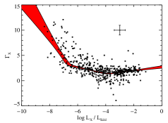
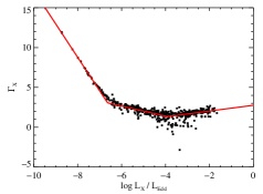
Figure 2: The measured values of $\Gamma_{X}$ and $\log L_{X}/L_{Edd}$ compared with the region containing $68\%$ of the posterior probability for the mean value of $\Gamma_{X}$ at fixed $L_{X}/L_{Edd}$ (left). The data point with error bars is not real and only used to illustrate the typical size of the error bars. Also shown are the posterior mean values for the true values of $\Gamma_{X}$ and $\log L_{X}/L_{Edd}$, compared with the best-fitting segmented line (right). A non-linear trend is apparent in both the segmented line model and in the estimated distribution of $\Gamma_{X}$ and $\log L_{X}/L_{Edd}$ using the segmented line as a prior.

The region containing $68\%$ of the posterior probability on the mean value of $\Gamma_{X}$ as a function of $L_{X}/L_{Edd}$ is also shown in Figure 2a. The location of the knots are estimated to be $\log L_{X}/L_{Edd}=-6.65\pm 0.25$ and $-3.91\pm 0.21$, respectively. The segmented line model of $\Gamma_{X}$ at fixed $L_{X}/L_{Edd}$ is preferred over a simple line model, illustrating the complex dependence of $\Gamma_{X}$ on $L_{X}/L_{Edd}$. In Figure 2b I show the posterior mean values of $\Gamma_{X}$ and $\log L_{X}/L_{Edd}$, as well as the segmented line computed from the posterior mean for its parameters. The posterior mean estimates for the true (i.e., not measured) values of $\Gamma_{X}$ and $\log L_{X}/L_{Edd}$ represent a more model-independent estimate of the dependence of the photon index on $L_{X}/L_{Edd}$. This represents a real advantage of the Bayesian approach, as not only are we able to estimate the probability distribution of the parameters of interest, but we can also estimate the probability distribution of the true values of the data as well, conditional on our assumed statistical model, the measured values of the data, and the amplitude of the measurement errors. The non-linear trend is also apparent from the values of $\Gamma_{X}$ and $L_{X}/L_{Edd}$ estimated from the Bayesian method. The knot at $L_{X}/L_{Edd}\sim 2\times 10^{-7}$ may represent the increasing prevalence of additional astrophysical components to the X-ray spectrum as the AGN becomes faintier, such as hot gas not associated with the AGN, while the knot at $L_{X}/L_{Edd}\sim 10^{-4}$ may represent a change in the accretion flow geometry. Figure 2b suggest that the scatter in $\Gamma_{X}$ at fixed $L_{X}/L_{Edd}$ increases near the knot at $L_{X}/L_{Edd}\sim 10^{-4}$, which may be indicative of instabilities when the accretion flow changes geometry, or of uncorrected intrinsic absorption. Further analysis of this data set will be discussed in Constantin et al. (2011, in prep).

6 Outstanding Issues in Measurement Error Models for Astronomical Data: Directions for Future Research

I will conclude by listing a couple of unsolved problems in dealing with measurement errors in astronomical data analysis, which I hope will lead to further research in this area.

• Data Subject to Large, Non-Gaussian Measurement Errors. Non-gaussian errors are common in astronomical data, especially when one is analyzing a set of derived quantities. Often, the most physically-interesting quantities are those derived by fitting an astrophysical model to the measured flux values at various wavelengths. Often the unertainties in these derived quantities are large, skewed, or exhibit multiple modes. There is currently no well-established method for handling the measurement errors in this case, although Bayesian hierarchical models such as that proposed by van Dyk et al. (2009) hold promise.

• Handling Measurement Errors in Massive Astronomical Data Sets. Current and planned astronomical surveys will provide an explosion of data, allowing one to construct data sets with millions to billions of objects, each with multiple quantities measured. Many powerful methods developed for data mining will be applied to these data, potentially providing a powerful route to knowledge discovery. Unfortunately, all of the quantities obtained from these data sets will be measured with error, and most methods developed for data mining of massive data sets do not incorporate measurement error. This is especially a problem when dealing with derived quantities, which will likely require a more careful statistical analysis on account of their sometimes highly irregular error distributions. Currently, algorithms, such as MCMC, that allow one to perform reliable statistical inference on complicated statistical models do not scale well to massive data sets. If we want to perform inference on massive data sets subject to measurement error using more complicated and realistic statistical models, we will need advances on the computational side.

I would like to thank Anca Constantin for sharing her data set with me before publication, and Aneta Siemiginowska, Xiaohui Fan, and Tommaso Treu for helpful comments on an earlier version of this manuscript. I acknowledges support by NASA through Hubble Fellowship grant #HF-51243.01 awarded by the Space Telescope Science Institute, which is operated by the Association of Universities for Research in Astronomy, Inc., for NASA, under contract NAS 5-26555.

References

- (1) Akritas, M. G., & Bershady, M. A. 1996, T. Astrophys. J., 470, 706
- (2) Andreon, S. 2006, Monthly Notic. of the Royal Astron. Soc., 369, 969
- (3) Bevington, P. R., & Robinson, D. K., Data Reduction and Error Analysis for the Physical Sciences, 3rd edn. (McGraw-Hill, New York, 2003)
- (4) Bovy, J., Hogg, D. W., & Roweis, S. T. 2009, arXiv:0905.2979
- (5) Carroll, R. J., Roeder, K., & Wasserman, L., 1999, Biometrics, 55, 44
- (6) Carroll, R. J., Ruppert, D., Stefanski, L. A., Crainiceanu, C. M., Measurement Error in Nonlinear Models: A Modern Perspective, 2nd edn. (Chapman & Hall/CRC, Boca Raton, 2006)
- (7) Cheng, C-L., & Van Ness, J. W., Statistical Regression with Measurement Error (Arnold, London, 1999)
- (8) Cheng, C-L., & Riu, J. 2006, Technometrics, 48, 511
- (9) Fuller, W. A., Measurement Error Models (John Wiley & Sons, New York, 1987)
- (10) Gelman, A., Carlin, J. B., Stern, H. S., & Rubin, D. B., Bayesian Data Analysis, 2nd edn. (Chapman & Hall/CRC, Boca Raton, 2004)
- (11) Huang, X., Stefanski, L. A., & Davidian, M. 2006, Biometrika, 93, 53
- (12) Kashyap, V. L., van Dyk, D. A., Connors, A., Freeman, P. E., Siemiginowska, A., Xu, J., & Zezas, A. 2010, T. Astrophys. J., 719, 900
- (13) Kelly, B.C. 2007, T. Astrophys. J., 665, 1489
- (14) Lee, H., et al. 2011, T. Astrophys. J., 731, 126
- (15) Little, R. J. A., & Rubin, D. B. Statistical Analysis with Missing Data, 2nd ed. (John Wiley & Sons, Hoboken, 2002)
- (16) Liu, J.S., Monte Carlo Strategies in Scientific Computing, (Springer, New York, 2004)
- (17) Patriota, A. G., & Bolfarine, H. 2008, T. Indian J. of Stat., 70, 267
- (18) Patriota, A. G., Bolfarine, H., & de Castro, M. 2009, Statist. Method., 6, 408
- (19) Press, W. H., Teukolsky, S. A., Vetterling, W. T., & Flannery, B. P., Numerical Recipes: The Art of Scientific Computing, 3rd edn. (Cambridge Unv. Press, New York, 2007)
- (20) Robert, C. P., & Casella, G., Monte Carlo Statistical Methods, 2nd edn. (Springer, New York, 2004)
- (21) Roy, S., Banerjee, T., 2006, Ann. Instit. Statist. Math., 58, 153
- (22) Sprent, P. 1966, J. Royal Stat. Soc. Ser. B, 28, 278
- (23) Tremaine, S., et al. 2002, T. Astrophys. J., 574, 740
- (24) van Dyk, D. A., Connors, A., Kashyap, V. L., & Siemiginowska, A. 2001, T. Astrophys. J., 548, 224
- (25) Van Dyk, D. A., DeGennaro, S., Stein, N., Jefferys, W. H., & von Hipple, T. 2009, T. Ann. of App. Stat., 3, 117
- (26) Yu, Y., & Meng, X-L. 2011, J. of Comput. & Graph. Stat., 20, 531