On The Apparent Narrowing of Radio Recombination Lines at High Principal Quantum Numbers

Abstract

We critically analyze the Bell et al. findings on “anomalous” widths of high-order Hydrogen radio recombination lines in the Orion Nebula at 6 GHz. We review their method of modified frequency switching and show that the way this method is used for large $\Delta n$ is not optimal and can lead to misinterpretation of measured spectral line parameters. Using a model of the Orion Nebula, conventional broadening theory, and Monte Carlo simulation, we determine a transition zone $n=224,\,\ldots,\,241$ ($\Delta n=11,\,\ldots,\,14$), where measurement errors grow quickly with $n$ and become comparable with the measurement values themselves. When system noise and spectrum channelization are accounted for, our simulation predicts “processed” line narrowing in the transition zone similar to that reported by Bell et al. We find good agreement between our simulation results and their findings, both in line temperatures and widths. We conclude, therefore, that Bell et al.’s findings do not indicate a need to revise Stark broadening theory.

1. Introduction

In the 1990s, Morley Bell and coauthors developed a technique for measuring weak spectral lines by reducing broad baseline variations (Bell 1997). This technique was referred to as “modified frequency switching” and was used to detect of weak atomic and molecular/maser lines in spectra of gaseous nebulae, circumstellar envelopes, and star formation regions (see, e.g., Bell & Feldman 1991, Bell et al. 1992; 1993).

Bell and coauthors used this technique to measure radio recombination line (RRL) widths and temperatures (Bell et al. 2000, hereafter BASV). At 6 GHz, they found that the “…[processed H] lines at large n are both narrower and stronger than expected from theory…” and suggested, “This behavior is … inconsistent with Griem’s theory …”. This publication, with its subtitle: “Confrontation with theory at high principal quantum numbers” induced a wave of publications where BASV’s finding was called an “anomaly”, “puzzle” and even “mystery”. For example, Oks 2004 paper is titled “On the puzzle of the observed narrowing of radio recombination lines,” Griem 2005 concludes his paper by writing that the result “…remains a mystery…,” Gavrilenko & Oks 2007 calls the result a “dramatic discrepancy,” and Watson 2006 concludes his abstract with “Thus this mystery is not resolved by the present calculations”.

While some authors have sought an explanation of these findings in the revision of Stark broadening theory (e.g., Oks 2004, Watson 2006), some remain skeptical about the modified frequency switching technique or suggest that it requires verification. For example, von Procházka et al. 2010 writes “…it is easy to distort the RRL line shape using data reduction techniques (Bell et al. 2000).” Griem 2005 referred to private communication with Bell stressing that “…measurement errors related to large reduction factors from unprocessed to processed Voigt profile widths can probably not be excluded (M. B. Bell 2004, private communication)”. In their book, Gordon & Sorochenko 2009 concluded: “The Bell et al. (2000) results are so different from what had been expected, and the observing technique is so new, that we suggest waiting for an independent confirmation of the observations before accepting a fault in the present theory of RRL Stark broadening.”

BASV’s findings are based on frequency switched or “processed” observational data, which were recently presented in Bell et al. 2011 and re-interpreted in Bell 2011. Their findings result from recursive frequency switching, in software, of observational data that were initially recorded at the telescope using hardware frequency switching.

In this paper, we investigate the frequency switching technique and demonstrate that, if applied correctly, it has a number of advantages. Frequency switching removes many gain variations and does not require subjective estimates of the zero level of a spectrum. Though the technique helped BASV to detect RRLs with $\Delta n$ greater than $\Delta n=6$ (Smirnov et al. 1984), the way the method was used was not optimal and, as such, cannot be used to test the theory of spectral line broadening. We present simulations based on the Lockman & Brown 1975 model of the Orion Nebula and conventional theory of spectral line broadening. We apply observational specifications from BASV and Bell et al. 2011, including frequency range, channel width, frequency switching offset, number of frequency switching overlaps, and noise temperature rms. Results of our simulation demonstrate good agreement with BASV’s findings, both in line width and temperature. The computed “processed” widths exhibit narrowing similar to that reported in BASV. We show that BASV’s spectral line “narrowing” is the result of the way the observational data were processed and that BASV’s findings do not contradict the existing Stark broadening theory.

2. Software Frequency Switching

In this section, we introduce the data reduction technique used by BASV to systematically acquire information about weak spectral features in the presence of baseline fluctuations. Bell 1997 established and named this technique SOFMOR (“small-offset frequency-switching multiple overlap reduction”). This technique was then called “modified frequency switching” (MFS) in BASV. SOFMOR and MFS are frequency switching techniques that use a frequency offset fixed in the receiver hardware (see, e.g., Robinson 1964), followed by recursive frequency switching in software. Here, we refer to this technique (whether conducted in hardware or software) as FS (frequency switching).

In FS, the original spectrum is subtracted from a copy which is shifted by a number of channels (an offset). Mathematically, it can be related to a finite difference iteration.

If the offset is $h$, then the notation

$$f_{p}=f(x+p\,h)$$ (1)

can be used. Formulae for the results of $m$ FS iterations ($m$ finite differences) are then

$$f^{(1)} = f_{1}-f_{0}$$

$$f^{(2)} = f_{2}-2f_{1}+f_{0}$$

$$f^{(3)} = f_{3}-3f_{2}+3f_{1}-f_{0}$$

$$f^{(4)} = f_{4}-4f_{3}+6f_{2}-4f_{1}+f_{0}$$

and so on (see, e.g., Beyer 1987, p. 449; Zwillinger 2002, p. 705), therefore

$$f^{(m)}=\sum_{k=0}^{m}f_{k}{m\choose k}(-1)^{m+k}\quad.$$ (2)

When $f(x)$ is given with uncertainty $\pm\sigma_{0}$, where $\sigma_{0}$ is standard deviation, the resulting uncertainty in $f^{(m)}$ can be derived from the error propagation rule (see, e.g., Taylor 1997, p. 75) as

$$\sigma_{m}=\sigma_{0}\sqrt{\sum_{k=0}^{m}\left(\frac{\partial f^{(m)}}{\partial f_{k}}\right)^{2}}=\sigma_{0}\sqrt{\sum_{k=0}^{m}{m\choose k}^{2}}=\sigma_{0}\sqrt{{2m\choose m}}.$$ (3)

Given that an FS spectrum overlaps with itself, the case of dependent samples must be applied (see below).

If $f(x)$ is a single channel feature (digital analogue of $\delta$-function), that is

$$f(x)=\delta(x_{0})=\left\{\begin{array}[]{ll}1,&\;\;x=x_{0}\\ 0,&\;\;{\rm{otherwise,}}\end{array}\right.$$

following Equation (2), $m$ FS-overlaps generates a series of equidistant peaks with amplitudes ${m\choose k}(-1)^{m+k}$. This is illustrated in the following Pascal’s triangle for six consecutive overlaps or three cycles:

overlap, m														cycle, i
0							1							0
1						-1		1
2					1		-2		1					1
3				-1		3		-3		1
4			1		-4		6		-4		1			2
5		-1		5		-10		10		-5		1
6	1		-6		15		-20		15		-6		1	3

.

Each cycle of two overlaps results in a symmetric pattern with a prominent central feature. The amplitude of the central feature after $i$ FS-cycles is the central binomial coefficient:

$$|A_{i}|={2i\choose i}=2,\;6,\;20,\;{\rm\dots}\hskip 19.91684pt(i=1,\;2,\;3,{\rm\dots})\quad.$$ (4)

According to Equation (3), the standard deviation after $i$ FS-cycles

$$\sigma_{i}=\sqrt{{4i\choose 2i}}=\sqrt{6},\;\sqrt{70},\;\sqrt{924},\;{\rm\dots}\hskip 19.91684pt(i=1,\;2,\;3,\;4,{\rm\dots})\;,$$ (5)

resulting in a signal-to-noise ratio (S/N) of

$${\rm S/N}_{i}=\frac{{2i\choose i}}{\sqrt{{4i\choose 2i}}}=0.82,\;\;0.72,\;\;0.66,\;{\rm\dots}\hskip 19.91684pt(i=1,\;2,\;3,{\rm\dots})\;.$$ (6)

Using Stirling’s formula (see, e.g., Abramowitz & Stegun 1965) we obtain

$${\rm S/N}_{i}\approx\left(\frac{2}{\pi i}\right)^{1/4}=0.89\;i^{-1/4}\quad.$$ (7)

Therefore, BASV’s S/N tends to decrease with the number of FS-cycles, $i$, as $i{}^{-1/4}$ .

When independent samples are superimposed, the standard deviation is scaled as $\sigma_{i}=2,\;4,\;8,\ldots$ , which results in the growth of the S/N: ${\rm S/N}_{i}={2i\choose i}/2^{i}=1,\;1.5,\;2.5,\;\ldots\;$ ($i=1,\;2,\;3,\;\ldots$). This common approach is not applicable to the FS technique used in BASV. Instead, they overlap the once recorded spectrum with itself and therefore the case of dependent samples must be used, as derived in Equations (5)–(7).

Though the first overlap in BASV occurs in hardware, where two independent samples are mixed, the S/N remains unchanged because the first overlap of two samples produces a $\sqrt{2}$ increase in the resulting standard deviation regardless of whether the two samples are dependent (software FS) or independent (hardware FS).

Figure 1 shows a Gaussian feature characterized by its full width at half-maximum (FWHM), $w$, and its transformation after 2, 4, and 6 FS-overlaps are applied to the initial feature. The frequency offset or FS-offset, h, is chosen to be much greater than the width, $h\gg w$. Additional features appear offset from the central feature, whose offsets are multiples of $h$. All the features are shifted relative to the position of the original feature, $x_{0}$. After i FS-cycles, the central feature is located at $x=x_{0}-i\,h$. These shifts are removed in Figures 1 and 2, such that all features are centered vertically. Additionally, all features are normalized and inverted (where necessary) to compare their shapes and widths.

If $h\gg w$, the additional features (referred to as “reference images” in Bell 1997) can be removed by adding or subtracting scaled versions of the central feature to them—a process referred to as “cleaning” in Bell 1997. For example, after two FS-overlaps, the additional features shown in Figure 1 can be removed by adding the central feature divided by 2. Dividing this result by $-2$ recovers the original feature exactly. After four overlaps, shown in Figure 1, the additional features are removed by adding $-1/6$ and $4/6$ of the central feature to them. Dividing the central feature by 6 recovers the original feature exactly.

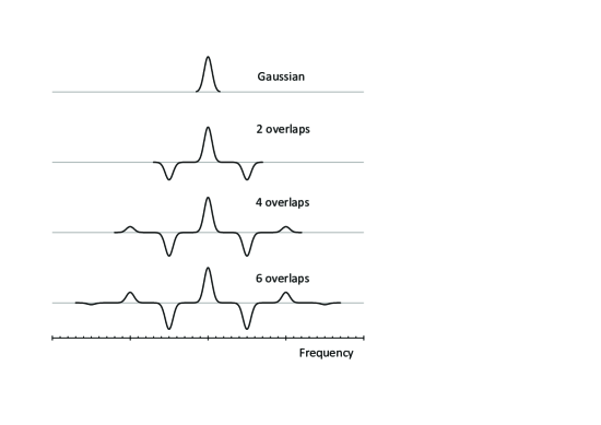
Figure 1.— Transformation of a Gaussian shape after 2, 4, and 6 FS-overlaps. The initial width, $w$, is much less than the FS offset, $h$; $w/h=0.2$. This plot is a graphical depiction of Pascal’s triangle in Section 2. To compare the shapes and widths, we invert (where necessary) the resulting spectra and normalize the peak intensity of the central feature to the intensity of the initial Gaussian.

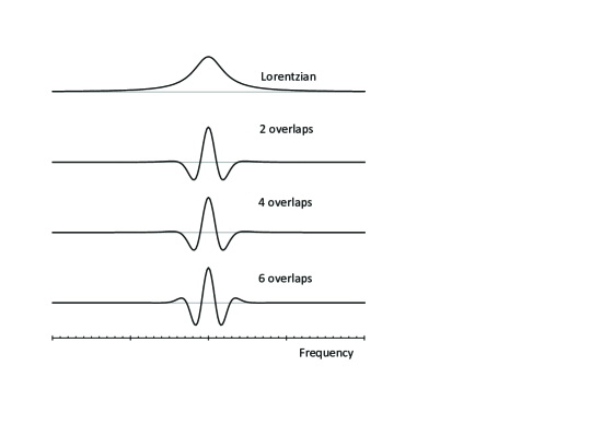
Figure 2.— Transformation of a Lorentzian shape after 2, 4, and 6 FS overlaps. The initial width, $w$, is greater than the offset, $h$. The ratio $w/h=4$ is used, which corresponds to BASV’s $\Delta n=20$ case. To compare the shapes and widths, we invert (where necessary) the resulting spectrum and normalize the peak intensity of the central feature to the intensity of the initial Lorentzian.

This normalization procedure keeps the central feature’s amplitude unchanged regardless of the number of FS-cycles, $i$. However, according to Equation (7), the noise level grows as $i{}^{1/4}$ .

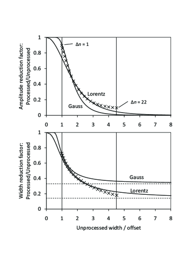
Figure 3.— Reduction factors (processed over unprocessed) for the peak line temperature (top plot) and the line width (bottom plot) as a function of the normalized unprocessed width, $w/h$. Both plots are calculated for six FS-overlaps. Vertical lines show minimal and maximal values of $w/h$ for BASV’s observations: $1\lesssim w/h\lesssim 4.5$. Crosses show reduction factors predicted by the three-component Orion Nebula model of Lockman & Brown 1975. Horizontal dashed lines in the bottom plot are the asymptotes for Gaussian and Lorentzian curves as $w/h\rightarrow\infty$. These plots demonstrate that, for a fixed FS-offset h, significant reduction in spectral line intensity and width results from FS as the unprocessed line width increases due to Stark broadening.

NRAO’s 140 ft telescope was used by BASV to observe the Orion Nebula at 6 GHz. Based on the 140 ft data archive of the 1992 April observation (integration time of $\sim\!48$ hours, system temperature of $\sim\!120\,\textrm{K}$, and channel width of $\sim\!78\,\textrm{kHz}$), a noise temperature $T_{\textrm{rms}}\approx 1\,\textrm{mK}$ could be achieved. Given that BASV used six overlaps (one hardware and five software FS-overlaps) or three cycles, Equation (7) implies an “frequency-switched” temperature rms of $T_{\textrm{rms}}\approx 1.5\,\textrm{mK}$.

Figure 2 illustrates the case when the FS-offset is less than the original line width, $h<w$, specifically $h=w/4$. This figure shows the transformation of a Lorentzian feature after 2, 4, and 6 FS-overlaps. To compare the shapes and widths, we normalize the peak intensity of the central feature to the intensity of the initial feature. Figure 2 shows that the central feature of the processed line is much narrower than the width of the original Lorentzian. Given that FS processing reduces line widths and amplitudes when $h<w$, BASV refer to them as “processed” widths and amplitudes.

The Voigt profile, which models the RRL shape, is a convolution of Gaussian and Lorentzian profiles, where the Gaussian represents the Doppler-broadened contribution and the Lorentzian represents the impact-broadened contribution (Gordon & Sorochenko 2009). Figure 3 shows how the amplitudes and widths of FS-processed Gaussian and Lorentzian profiles vary as a function of the normalized unprocessed width, $w/h$. These plots show amplitude and width reduction factors (processed to unprocessed ratio) calculated for six FS-overlaps. The vertical lines show the limits of BASV’s experiment: $1\lesssim w/h\lesssim 4.5$. Crosses are reduction factors predicted by the Lockman & Brown 1975 Orion Nebula model (see the next section). Horizontal dashed lines in the bottom plot are the asymptotes for Gaussian and Lorentzian cases as $w/h\rightarrow\infty$.

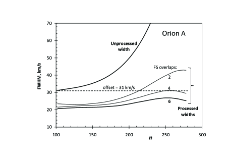
Figure 4.— Processed width vs. $n$ for different number of FS overlaps at 6 GHz. Simulation is conducted for the Orion Nebula model of Lockman & Brown 1975; no noise is taken into account. Dashed line shows BASV’s FS-offset (eight channels = 31.2 km s^-1). The upper (thick) curve shows the unprocessed width $w$ vs. $n$. The lower curve corresponds to the BASV’s case of six FS-overlaps. This plot demonstrates that when $h<w$, the processed width is increasingly insensitive to the significantly changing unprocessed width as the number of overlaps increase. This indicates that the FS technique in BASV’s case is a poor probe of line broadening.

3. Application of FS to Model Spectra

The frequency switching technique used in BASV consists of two independent steps: (1) overlapping the spectrum and (2) “cleaning” the overlapped spectrum. Overlapping six times creates a set of “reference images” for each line feature in the spectrum. The result of overlapping (step 1) is illustrated in Figures 1 $(h\gg w$) and 2 ($h<w$). When $h<w$ (BASV’s case), overlapping reduces the line widths to below the FS-offset, $h$.

After overlapping, the reference images are removed. In Bell (1997) and BASV, this “cleaning” procedure was done manually, one line at a time, starting with the strongest line and working to the weakest. BASV’s reported line widths after cleaning are in the range of 18 to 30 km s^-1, which is less than or about the Doppler width and less than the FS-offset (Figures 2 and 4 in BASV). The conclusion made in BASV about line “narrowing” is based on interpretation of these “processed” widths.

A multi-component non-LTE radiative transfer simulator was created to explore the effect of FS on model RRL spectra. For the Orion Nebula we use the three-component model of Lockman & Brown 1975, which simulates the beam size of the 140 ft radio telescope. The model consists of a compact (0.043 pc) dense ($N_{e}=10^{4.5}\,\textrm{cm}{}^{-3}$) symmetric core located behind two extended (0.56 and 2.50 pc) layers of gas of lower density ($N_{e}=10^{3.5}$ and $10^{2.3}\,\textrm{cm}{}^{-3}$). The corresponding temperatures are $T_{e}=$7500 K (core), 10,000 K, and 12,500 K (outer layer). This model predicts continuum emission and H$n\alpha$ and H$n\beta$ spectra in agreement with observations between 1 and 90 GHz (Lockman & Brown 1975).

Figures 4–6 show the model results for processed line temperatures and processed widths versus principal quantum number, $n$, for the Orion Nebula model at 6 GHz. To avoid ambiguity associated with the cleaning procedure, we process each modeled spectral line separately. The processed line width is the FWHM of the central feature measured above the zero level (see Figure 2).

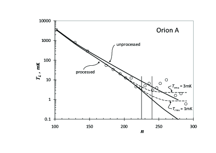
Figure 5.— Line temperature, $T_{L}$, vs. $n$ for the Orion Nebula at 6 GHz. Open circles represent line temperatures obtained by BASV: processed line temperatures after six FS-overlaps (Bell et al. 2011). The theoretical curves result from Lockman & Brown 1975 model. Upper and lower solid curves show unprocessed and processed line temperatures from the model spectra without noise. Upper and lower dashed curves show processed line temperatures from model spectra with 3 and 1 mK noise, correspondingly. Vertical lines are positioned at $n$ values corresponding to theoretical processed temperatures $T_{L}=3\>\textrm{mK}$ (left) and $T_{L}=1\>\textrm{mK}$ (the right vertical line). This plot indicates that our model of processed line temperatures agrees with BASV’s findings for $(n,\Delta n)\lesssim(224,11)$. Above this limit, our model suggests BASV’s results are dominated by noise fluctuations.

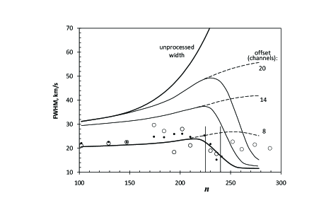
Figure 6.— Processed width (six FS-overlaps) vs. $n$ computed for different FS-offsets (8, 14, and 20 channels) for the Orion Nebula model at 6 GHz. Dashed curves—no noise; solid curves—1 mK noise added to model spectra. Open and filled circles show the processed widths obtained by BASV for the Orion Nebula and W51. The upper thick solid curve shows the unprocessed width vs. $n$. Vertical lines are positioned at $n$ values corresponding to theoretical processed temperatures $T_{L}=3\>\textrm{mK}$ and $T_{L}=1\>\textrm{mK}$ (see Figure 5). The lower thick solid curve corresponds to BASV’s eight-channel FS-offset and 1 mK noise fluctuations. It agrees well with BASV’s processed findings for $(n,\Delta n)\lesssim(241,14)$. In the transition zone (between the two vertical lines), the modeled width behavior imitates “narrowing” of the processed spectral lines reported by BASV.

Figure 4 shows the processed widths (FWHM) for 2, 4, and 6 FS-overlaps (1, 2, and 3 cycles). Following BASV, we used six overlaps and an offset of 625 kHz = 31.2 km s^-1, which corresponds to eight spectral channels (channel width of 78.13 kHz = 3.9 km s^-1). Noise was not added to the model spectra when computing these curves. The dashed line shows BASV’s FS-offset (eight channels = 31.2 km s^-1). After six FS-overlaps, the processed width (FWHM) remains at the level of $\sim\!\!70\%,\,\ldots,\,85\%$ of the offset, reaching a maximum at $n\simeq 260$, then drops down to 81% at higher $n$. This behavior reflects a growing contribution to the line shape from the nebula’s low-density outer layer at very high $n$. The greater contribution of the outer low-density layer at high $n$ also explains the deviation of the reduction factors (crosses) in Figure 3 from the “Lorentzian” behavior.

Figure 5 shows the line temperature, $T_{L}$, versus $n$ for the Orion Nebula. Open circles are BASV’s processed $T_{L}$. Solid curves show unprocessed (upper curve) and processed $T_{L}$ for the model spectra without noise. Dashed curves show processed $T_{L}$ for model spectra with 1 and 3 mK noise added. These curves are obtained using the following Monte Carlo method. For each modeled spectral line feature, normally distributed noise is added, then FS-overlapped six times. $T_{L}$ and $w$ of this processed feature are then estimated by a Gaussian fit, as done by BASV. The least-squares-fitting algorithm searches for the best fit within a $\pm 2$ channel interval about the central line frequency. These steps were trialed 1000 times to determine the mean and standard deviation values of $T_{L}$ and $w$ for each processed spectral line feature. This method was carried out for the expected 1 mK noise rms and, additionally, a 3 mK noise rms. Two vertical lines in Figure 5 are positioned at $n$ values corresponding to the processed, noise-free model temperatures $T_{L}=3\>\textrm{mK}$ (left line) and $T_{L}=1\>\textrm{mK}$ (right line). Given BASV’s $\,T_{{\rm rms}}\sim 1\>\textrm{mK}$, the vertical lines represent the $3\sigma$ and $1\sigma$ limits. The corresponding limiting values of $n=224$ ($\Delta n=11$) and $n=241$ ($\Delta n=14$) are also indicated by vertical lines in Figure 6.

Processed widths versus n for 8, 14, and 20 channel offsets are shown in Figure 6 for the 6 GHz Orion Nebula model. For comparison, the thick upper solid curve is unprocessed noise-free model widths. Dashed curves in Figure 6 correspond to processed noise-free model widths, while solid curves are the corresponding processed widths resulting from the Monte Carlo method described above using 1 mK noise added to the model spectra. Open and filled circles in Figure 6 are BASV’s processed widths for the Orion Nebula and W51 (see also Bell et al. 2011). The left and right vertical lines show the $3\sigma$ and $1\sigma$ confidence limits from Figure 5.

4. Discussion

The multiple frequency switching technique reduces amplitudes of broad baseline variations and therefore can be used to systematically “flatten” baselines (Bell & Feldman 1991, Bell et al. 1992; 1993). Compared to standard spline/polynomial baseline fitting, which allows for subjective decisions, the FS technique reduces baseline variations objectively. For spectral features that are much wider than the offset, $h$, FS can be likened to differentiation, which acts as a high-pass filter in the frequency domain (see, e.g., Hamming 1998, Owen 1995). In this case, six overlaps approximates the sixth derivative with respect to frequency, which makes FS an efficient high-pass filter. This not only reduces broad variations in the spectrum, but in BASV’s case (six overlaps, $h<w$ ), it also reduces broad spectral line wings larger than the FS-offset, which manifests as line narrowing (see, e.g., Figure 2).

We use the Lockman & Brown 1975 model of the Orion Nebula and simulate the conditions of BASV’s observations at 6 GHz: telescope beam size, frequency range, channel width, offset, number of overlaps, and noise temperature. When modeling, we can avoid some difficulties that BASV faced when they processed the real spectrum. The real spectrum is abundant with spectral lines; after overlapping six times, the resulting spectrum is crowded with lines and reference lines. This situation is further complicated when significant noise fluctuations are present, which is BASV’s case when $\Delta n>11$, so cleaning becomes a non-trivial and subjective procedure. In our case cleaning is trivial as we can model and clean each RRL individually, with and without noise.

For all $\textrm{H}n\Delta n$ lines studied in BASV, the unprocessed width (i.e., before FS) is greater than the FS-offset used. We show that the processed width weakly depends on $n$ and $\Delta n$ (see Figure 4, the six FS-overlaps case). In fact, it remains about $0.8\,h$ for a wide range of $n$ and $\Delta n$. This property of the FS technique makes it insensitive to changes in RRL widths when $h<w$. (It is for this reason that we justify the inclusion of BASV’s processed widths for W51 at 6 GHz in Figure 6.) The FS technique can be used to systematically eliminate broad baseline variations to detect weak lines, however, in BASV’s case (six overlaps, $h<w$), this technique is not well suited to study RRL broadening. If one’s purpose is to test the theory of spectral line broadening, the choice of the offset made in BASV ($h<w$) is not optimal.

It is shown in the previous sections that FS reduces the S/N (see Equation (6)) and spectral line amplitudes (Figure 3). As a result of amplitude reduction, the processed line temperature drops rapidly to the noise temperature $T_{\textrm{rms}}=1$ mK as $n$ and $\Delta n$ grow (the lower solid curve in Figure 5). The model processed line amplitude reaches 3 mK ($3\sigma$ level) at $n=224$ ($\Delta n=11$) and 1 mK ($1\sigma$ level) at $n=241$ ($\Delta n=14$). The interval between $n=224$ and 241 (between $\Delta n=11$ and 14) is a transition zone between observable spectral lines and noise. Figure 6 shows that the processed width behavior in the transition zone imitates “narrowing” of the processed spectral lines observed by BASV in spectra of the Orion Nebula and W51 at 6 GHz. This “narrowing” is the result of “forcing” a program to fit Gaussians to features dominated by noise fluctuations—the procedure used by BASV.

Spectra presented in Bell 1997, BASV and Bell et al. 2011 result from the overlapping and cleaning steps explained in Section 3. Though BASV applied overlapping to the entire spectrum, cleaning was applied selectively to features located near the expected spectral line frequencies, even if the processed line temperatures were below $3\,\sigma$. This subjective and selective approach could create “spectral lines” from random fluctuations at the $\lesssim 3\,\sigma$ level, which are abundant in the spectrum.

For $\Delta n\geq 14$ the width errors predicted by our Monte Carlo simulation are comparable to the widths themselves. Therefore, BASV’s data points for $\Delta n\geq 14$ shown in Figures 5 and 6 are likely to be misinterpreted noise features.

In conclusion, FS is a useful technique for detecting and measuring weak spectral features, if required corrections are minimal, that is if the FS offset is greater than the line width: $h\gtrsim w$. Based on our simulation results, we argue that BASV’s $T_{\textrm{rms}}\approx 1$ mK observations of hydrogen RRLs from the Orion Nebula at 6 GHz are limited to $\Delta n<14$. Within this limit, we find good agreement between their results and a Monte Carlo simulation based on conventional Stark broadening theory and, therefore, we argue that BASV’s findings do not necessitate a revision of RRL Stark broadening theory. We suggest that further tests of line broadening theory above this limit will require observations with sub-mK sensitivity and improved baseline stability.

References

- Abramowitz & Stegun 1965 Abramowitz, M., & Stegun, I. A. 1965, An Introduction to Error Analysis: The Study of Uncertainties in Physical Experiment, 2nd edn. (New York: Dover)
- Bell 2011 Bell, M. 2011, Ap&SS, 335, 451
- Bell 1997 Bell, M. B. 1997, PASP, 109, 609
- Bell et al. 2011 Bell, M. B., Avery, L. W., MacLeod, J. M., & Vallée, J. P. 2011, Ap&SS, 335, 451
- Bell et al. 2000 Bell, M. B., Avery, L. W., Seaquist, E. R., & Vallée, J. P. 2000, PASP, 112, 1236
- Bell et al. 1993 Bell, M. B., Avery, L. W., & Watson, J. K. G. 1993, ApJS, 86, 211
- Bell & Feldman 1991 Bell, M. B., & Feldman, P. A. 1991, ApJ, 367, L33
- Bell et al. 1992 Bell, M. B., Feldman, P. A., & Avery, L. W. 1992, ApJ, 396, 643
- Beyer 1987 Beyer, W. H. 1987, CRC Standard Mathematical Tables, 28th edn. (Boca Raton, FL: CRC Press)
- Gavrilenko & Oks 2007 Gavrilenko, V. P., & Oks, E. 2007, Phys. Scr., 76, 43
- Gordon & Sorochenko 2009 Gordon, M. A., & Sorochenko, R. L. 2009, Radio Recombination Lines: Their Physics and Astronomical Applications (Astrophysics and Space Science Library) (New York: Springer)
- Griem 2005 Griem, H. R. 2005, ApJ, 620, L133
- Hamming 1998 Hamming, R. W. 1998, Digital Filters, 3rd edn. (Mineola: Courier Dover Publications)
- Lockman & Brown 1975 Lockman, F. J., & Brown, R. L. 1975, ApJ, 201, 134
- Oks 2004 Oks, E. 2004, ApJ, 609, L25
- Owen 1995 Owen, A. J. 1995, Uses of Derivative Spectroscopy, Tech. Rep. 5963-3940E, Agilent Technologies
- Robinson 1964 Robinson, B. J. 1964, ARA&A, 2, 401
- Smirnov et al. 1984 Smirnov, G. T., Sorochenko, R. L., & Pankonin, V. 1984, A&A, 135, 116
- Taylor 1997 Taylor, J. 1997, An Introduction to Error Analysis: The study of Uncertainties in Physical Experiment, 2nd edn. (Sausalito, CA: Univ. Science Books)
- von Procházka et al. 2010 von Procházka, A. A., Remijan, A. J., Balser, D. S., et al. 2010, PASP, 122, 354
- Watson 2006 Watson, J. K. G. 2006, J. Phys. B: At. Mol. Opt. Phys., 39, 1889
- Zwillinger 2002 Zwillinger, D. E. 2002, Difference Equations and Numerical Differentiation, 3.9 and 8.3.2 in CRC Standard Mathematical Tables and Formulae (Boca Raton, FL: CRC Press)