Influence of high permeability disks in an axisym-
metric model of the Cadarache dynamo experiment

Abstract

Numerical simulations of the kinematic induction equation are performed on a model configuration of the Cadarache von-Kármán-Sodium dynamo experiment. The effect of a localized axisymmetric distribution of relative permeability $\mu_{\rm{r}}$ that represents soft iron material within the conducting fluid flow is investigated. The critical magnetic Reynolds number ${\rm{Rm}}^{\rm{c}}$ for dynamo action of the first non-axisymmetric mode roughly scales like ${\rm{Rm}}_{\mu_{\rm{r}}}^{\rm{c}}-{\rm{Rm}}_{\infty}^{\rm{c}}\propto\mu_{r}^{-1/2}$ i.e. the threshold decreases as $\mu_{\rm{r}}$ increases. This scaling law suggests a skin effect mechanism in the soft iron disks. More important with regard to the Cadarache dynamo experiment, we observe a purely toroidal axisymmetric mode localized in the high permeability disks which becomes dominant for large $\mu_{\rm{r}}$. In this limit, the toroidal mode is close to the onset of dynamo action with a (negative) growth-rate that is rather independent of the magnetic Reynolds number. We qualitatively explain this effect by paramagnetic pumping at the fluid/disk interface and propose a simplified model that quantitatively reproduces numerical results. The crucial role of the high permeability disks for the mode selection in the Cadarache dynamo experiment cannot be inferred from computations using idealized pseudo-vacuum boundary conditions ($\mbox{\boldmath$H$}{\times}\mbox{\boldmath$n$}=0$).

1 Introduction

Astrophysical magnetic fields are a ubiquitous phenomenon. They affect formation and behavior of galaxies, stars or planets and might even be important for structure formation on cosmic scales. On astrophysical scales fluid flow driven field generation by virtue of the dynamo effect is relatively uncomplicated because the magnetic Reynolds number is always huge. However, due to their limited size the realization of dynamo action in laboratory experiments is a demanding task and requires an elaborate design that makes use of optimizations like an ideal guidance of a fluid flow or a selective choice of materials. Material properties like electrical conductivity or relative permeability have always been important for experimental dynamos. For example, the use of soft iron in the dynamo experiments of 1963Natur.198.1158L 1963Natur.198.1158L,1968Natur.219..717L was crucial for the occur-
rence of magnetic self excitation. More recently, the addition of high permeability mate-
rial (soft iron spheres) into a conducting fluid was examined to test magnetic self excita-
tion [2003PhRvE..67e6309D] in a flow that otherwise would not be able to sustain a dynamo.

The work presented here is motivated by the Cadarache von-Kármán-Sodium (VKS) dynamo [2007PhRvL..98d4502M]. In this experiment liquid sodium contained in a cylindrical vessel is driven by two counter–rotating impellers that are located close to the lids of the vessel. Dynamo action is obtained only when (at least one of) the flow driving impellers are made of soft iron with a relative permeability $\mu_{\rm{r}}\approx 65$ [2010NJPh...12c3006V]. Moreover the observed magnetic field is dominated by an axisymmetric mode [2009PhFl...21c5108M]. It can be conjectured that the occurrence of dynamo action with soft iron impellers and the axisymmetry of the magnetic field are linked but, so far, the very nature of the axisymmetric dynamo is still unknown.

A well-known necessary condition for the occurrence of dynamo action is a sufficiently complex conducting fluid flow that couples the toroidal and poloidal components of the magnetic field. The interaction between these components gives rise to the so-called dynamo cycle which consists of regenerating the toroidal field from the poloidal field and vice versa. This coupling can take place on large scales [1989RSPSA.425..407D] as well as on small scales by virtue of the well known $\alpha$-effect [1980mfmd.book.....K]. It is less well known that non-homogeneities in the electrical conductivity can also introduce such coupling and, by this, favour dynamo action. For example, a uniform flow over an infinite plate with varying conductivity can produce dynamo action [1992gafd...64..135B, 1993spd..conf..329W]. It is likely that inhomogeneous magnetic permeability can lead to dynamo action as well.

In this paper we investigate the impact of a localized disk-like permeability distribution embedded in a conducting axisymmetric fluid flow on the growth-rates of the first axisymmetric and non-axisymmetric magnetic eigenmodes. Induction effects due to non-axisymmetric perturbations (turbulence, small-scale or large-scale flow or conductivity/permeability distributions) are not taken into account. First, we briefly re-examine the threshold of the equatorial dipole mode as in 2010GApFD.104..505G and propose an explanation for the scaling law that relates the critical magnetic Reynolds number to the permeability in the impeller disks. Second we investigate the influence of the concentrated high permeability on the axisymmetric field modes. Even though they are always damped, according to Cowling’s theorem [1933MNRAS..94...39C, 1982GApFD..19..301H], for large $\mu_{\rm{r}}$ we find a dominant toroidal mode very close to the onset of dynamo action. We suggest that this eigenmode plays a significant role in the dominance of the axisymmetric mode in the dynamo observed in the VKS experiment [2007PhRvL..98d4502M].

2 Model

The induction equation with nonuniform material coefficients, i.e. spatially dependent electrical conductivity $\sigma=\sigma(\mbox{\boldmath$r$})$ and relative permeability $\mu_{\rm{r}}=\mu_{\rm{r}}(\mbox{\boldmath$r$})$, reads:

$$\frac{\partial\mbox{\boldmath$B$}}{\partial t}=\nabla\!\times\!\left(\!\mbox{\boldmath$u$}\!\times\!\mbox{\boldmath$B$}+\frac{1}{\mu_{\rm{r}}\mu_{0}\sigma}\frac{\nabla\mu_{\rm{r}}}{\mu_{\rm{r}}}\!\times\!\mbox{\boldmath$B$}-\frac{1}{\mu_{\rm{r}}\mu_{0}\sigma}\!\nabla\!\times\!\mbox{\boldmath$B$}\!\right),$$ (1)

where $u$ is the prescribed (mean) flow, $B$ the magnetic flux density and $\mu_{0}$ the vacuum permeability ($\mu_{0}=4\pi\times 10^{-7}\mbox{Vs/Am}$). The middle term in the right hand side of Eq. (1) proportional to $\sim\nabla\mu_{\rm{r}}\times\mbox{\boldmath$B$}$ represents the so-called ”paramagnetic pumping” [2003PhRvE..67e6309D]. This term is responsible for the suction of the magnetic field into the regions with large permeability and involves a (non divergence free) velocity-like field that we henceforth call ”pumping velocity”

$$\mbox{\boldmath$V$}^{\mu}=\frac{1}{\mu_{\rm{r}}\mu_{0}\sigma}\frac{\nabla\mu_{\rm{r}}}{\mu_{\rm{r}}}.$$ (2)

The eigenvalue problem associated with equation (1) is solved numerically by using two different methods. One is based on a spectral/finite element approach described in GLLNR11 (SFEMaNS, spectral/finite element method for Maxwell and Navier-Stokes equations) which solves the eigenvalue problem using ARPACK. The second approach utilizes a combined finite volume/boundary element method for timestepping equation (1), 2008giesecke_maghyd. Both approximation methods can account for insulating boundaries and non-uniform permeability and/or conductivity distributions. In the FV/BEM scheme insulating boundary conditions are treated by solving an integral equation on the boundary which allows a direct computation of the (unknown) tangential field components by correlating the (known) normal field components on the surface of the computational domain [iskakov2004, 2008giesecke_maghyd]. In the SFEMaNS code the magnetic field is computed numerically in a certain domain outside of the cylinder and matching conditions are used at the interfaces with the insulator [guermond2007].

The respective discretizations are done so that the transmission conditions across the material interfaces are satisfied. In addition to having passed independent convergence tests on manufactured solutions, the two codes have been cross-validated by comparing their outputs on various common test cases (see andregafd, andregafd, 2010GApFD.104..505G, 2010GApFD.104..505G and table 1 below).
We use the same configuration as applied in PhysRevLett.104.044503. The computational domain is inspired from the VKS configuration. The conducting fluid is contained in a cylinder of height $H=2.6$ and radius $R_{\rm{out}}=1.4$, surrounded by an insulator. The fluid fills two unconnected compartments. The moving fluid is contained in an inner cylinder of radius $R_{\rm{in}}=1$. The fluid contained in the annular region comprised between the cylinders of radius $R_{\rm{in}}=1$ and $R_{\rm{out}}=1.4$ is at rest; this region is referred to as the side layer (see figure 1). Two discoidal subdomains of radius $R_{\rm{imp}}=0.95$ are located in the intervals $z\in[-1.0;-0.9]$ and $z\in[0.9;1.0]$ and are meant to model soft iron impeller disks of thickness $d=0.1$; the relative magnetic permeability in these two disks is denoted $\mu_{\rm{r}}$. The velocity field $u$ and the permeability distribution $\mu_{\rm{r}}$ are assumed to be axisymmetric.

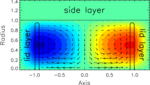
Figure 1: Velocity field used in the kinematic simulations. The azimuthal velocity, $u_{\varphi}$, is shown in color and the poloidal component of the velocity, $u_{r}\mbox{\boldmath$e$}_{r}+u_{z}\mbox{\boldmath$e$}_{z}$, is shown with arrows. The black structures in the intervals $z\in[-1.0;-0.9]$ and $z\in[0.9;1.0]$ represent two axisymmetric impellers of relative permeability $\mu_{\rm{r}}>1$. Note that the flow is mixed (poloidal and toroidal) between the two impeller disks and purely toroidal within and behind the impeller disks.

The velocity field between the impeller disks in the inner cylinder is given by the so-called MND fluid flow [2004phfl]:

$$u_{r}(r,z) = -(\pi/h)\cos\!\left({{2\pi z/h}}\right)r(1-r)^{2}(1+2r),$$

$$u_{\varphi}(r,z) = 4\epsilon r(1-r)\sin\left({{\pi z/h}}\right),$$ (3)

$$u_{z}(r,z) = (1-r)(1+r-5r^{2})\sin\left({{2\pi z/h}}\right),$$

where $h$ is the distance between the two impeller disks ($h=1.8$) and $\epsilon$ parametrizes the toroidal to poloidal ratio of the flow (in the following we choose $\epsilon=0.7259$) . A purely azimuthal velocity equal to the azimuthal velocity of the MND flow at $z=\pm h/2$ is assumed in the two impeller disks. A so-called lid layer [2005physics..11149S] is added behind each impeller disk, and the velocity field therein is modeled by linear interpolation along the $z$-axis between the azimuthal velocity at the outer side of the impeller disk and the no-slip condition at the lid of the vessel. The velocity field and the impeller disks (two thin structures shown in black solid lines) are displayed in figure 1. The conductivity is assumed to be uniform in the liquid metal and the soft iron disks. We focus in this paper on non-uniform permeability distributions only, which seems roughly justified for soft iron disks embedded in liquid sodium.

The equations are nondimensionalized so that $\mathcal{R}=R_{\rm{in}}$ is the reference length-scale ($R_{\rm{in}}$ is the radius of the flow active region) and $\mathcal{U}=\max[(u_{r}^{2}+u_{\varphi}^{2}+u_{z}^{2})^{\nicefrac{{1}}{{2}}}]$ is the reference velocity scale (maximum absolute value of the velocity field). The control parameter is the magnetic Reynolds number defined by ${\rm{Rm}}=\mu_{0}\sigma\mathcal{U}\mathcal{R}$.

3 Results

The eigenvalues of the differential operator in the right-hand side of equation (1) are denoted $\lambda=\gamma+i\omega$; the real part $\gamma$ is the growth-rate of the field amplitude ($\gamma<0$ corresponds to decay) and the imaginary part $\omega$ is the frequency. All the computations reported below give non-oscillatory eigen-modes (i.e. $\omega=0$). An immediate consequence of the axisymmetric setup is that the eigenmodes of the kinematic dynamo problem can be computed for each azimuthal wavenumber $m$.

3.1 Overview

Table 1: Comparison of growth-rates obtained with FV (hybrid finite volume/boundary element method) and SFEMaNS (spectral/finite element method for Maxwell and Navier-Stokes equations). $\rm{Rm}$ is the magnetic Reynolds number, $\mu_{\rm{r}}$ the disk permeability, $\gamma_{m0}^{\rm{t}}$ the growth-rate of the axisymmetric toroidal field, $\gamma_{m0}$ the growth-rate of the axisymmetric mixed field, $\gamma_{m1}$ the growth-rate of the first non-axisymmetric field ($m$1-mode). The thickness of the impeller disks is $d=0.1$.

${\rm{Rm}}$	$\mu_{\rm{r}}$	$\gamma_{m0}^{\rm{t}}$	$\gamma_{m0}$	$\gamma_{m1}$	Scheme
0	1	-8.950	-4.159	-4.273	FV
0	1	-8.977	-4.162	-4.322	SFEMaNS
0	60	-1.292	-3.887	-1.715	FV
0	60	-1.305	-3.893	-1.722	SFEMaNS
30	1	-8.748	-3.591	-2.690	FV
30	1	-8.770	-3.597	-2.780	SFEMaNS
30	60	-1.134	-3.404	-2.511	FV
30	60	-1.155	-3.478	-2.476	SFEMaNS
70	1	-8.079	-3.467	-0.119	FV
70	1	-8.119	-3.471	-0.215	SFEMaNS
70	60	-1.203	-3.232	1.012	FV
70	60	-1.219	-3.264	0.969	SFEMaNS

We show in table 1 sample values of growth-rates obtained by FV and SFEMaNS for the above simplified VKS model problem. This table confirms that FV and SFEMaNS converge to the same solutions up to $2\%$ on the growth-rates. We use the following notation in table 1 and in the rest of the paper: $\gamma_{m0}$ is the growth-rate of a mixed poloidal/toroidal mode. This mode degenerates to a purely poloidal mode when ${\rm{Rm}}=0$, and when there is no permeability jump (e.g. for stainless steel disks) this mode always determines the behavior of the axisymmetric field. Furthermore, $\gamma_{m0}^{\rm{t}}$ is the growth-rate of the first axisymmetric mode ($m=0$) that is purely toroidal and $\gamma_{m1}$ is the growth-rate of the first non-axisymmetric mode ($m=1$).

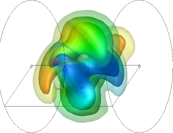
(a) ${\rm{Rm}}=30$, $\mu_{\rm{r}}=1$, $m=1$, decay

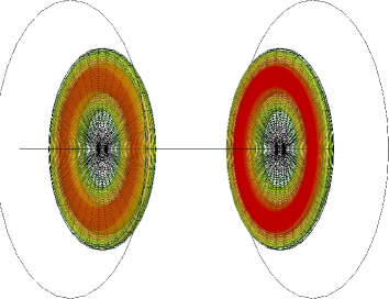
(b) ${\rm{Rm}}=30$, $\mu_{\rm{r}}=60$, $m=0$, decay

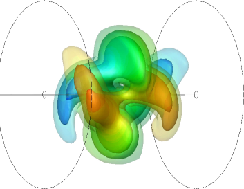
(c) ${\rm{Rm}}=70$, $\mu_{\rm{r}}=1$, $m=1$, decay

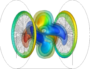
(d) ${\rm{Rm}}=70$, $\mu_{\rm{r}}=60$, $m=1$, growth

Figure 2: Dominant magnetic eigenmodes. The isosurfaces show the magnetic energy density at $10\%,20\%,40\%$ of the maximum value. The colors show $H_{\varphi}=\mu_{\rm{r}}^{-1}B_{\varphi}$ and the meshes show the location of the soft iron disks (in the right column). Note that all eigenmodes are decaying except the case ${\rm{Rm}}=70,\mu_{\rm{r}}=60$ (lower right panel) which is above the dynamo threshold and therefore presents a growing $m1$–mode.

When $\rm{Rm}=0$, the dominant and the second dominant $m0$-modes at $\mu_{\rm{r}}=1$ are purely poloidal and purely toroidal, respectively; the situation is reversed at $\mu_{\rm{r}}=60$: the dominant mode is purely toroidal. All growth-rates increase with $\mu_{\rm{r}}$. When $\rm{Rm}>0$, the growth-rate of the $m0$-mode is always negative in agreement with Cowling’s theorem [1933MNRAS..94...39C], but we observe that its relaxation time becomes longer as the permeability in the impeller disks increases. We also observe that dynamo action occurs on the $m1$-mode and that increasing $\mu_{r}$ lowers the critical threshold on $\rm{Rm}$.

Snapshots of the dominant magnetic eigenmode are shown in figure 2. The structure of the $m1$-mode does not change very much with respect to $\mu_{\rm{r}}$ and ${\rm{Rm}}$; it is an equatorial dipole with two opposite axial structures mainly localized in the bulk of the fluid. In contrast, the $m0$-mode is essentially localized in the two impeller disks and does barely differ from the pattern obtained in the free decay case (see figure 6 below).

3.2 Effect of the disk permeability on the $m1$-mode

Figure 3 shows the growth-rate of the $m1$-mode as a function of the relative permeability of the impeller disks for four values of the Reynolds number.

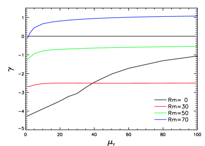
Figure 3: Growth-rate of the $m1$-mode as a function of $\mu_{\rm{r}}$ for ${\rm{Rm}}=0,30,50,70$.

This figure is similar to figure 13a in 2010GApFD.104..505G. The growth-rate reaches quickly an asymptotic value when $\rm{Rm}>0$, which is not the case when $\rm{Rm}=0$. The $m1$-mode clearly depends on ${\rm{Rm}}$ and exhibits dynamo action when ${\rm{Rm}}$ is large enough. It can be seen in the left panel in figure 4 that the threshold for dynamo action goes from ${\rm{Rm}}^{\rm{c}}\approx 76$ when $\mu_{\rm{r}}=1$ to ${\rm{Rm}}^{\rm{c}}_{\infty}\approx 53.95$ when $\mu_{\rm{r}}\rightarrow\infty$.

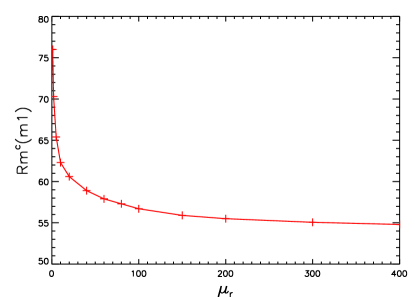
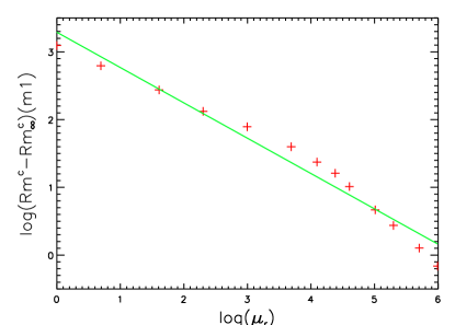
Figure 4: Left panel: Dynamo threshold for the $m1$-mode as a function of $\mu_{r}$. Right panel: Linear fit on $\log$-$\log$ scale provides the scaling ${\rm{Rm}}^{\rm{c}}-{\rm{Rm}}^{c}_{\infty}\propto\mu_{r}^{-0.52}$.

The asymptotic threshold for $\mu_{\rm{r}}\rightarrow\infty$ has been calculated by enforcing the boundary condition $\mbox{\boldmath$H$}{\times}\mbox{\boldmath$n$}=0$ on the impeller disks (pseudo-vacuum or Vanishing Tangential Field condition) while keeping the flow pattern (3) unchanged. This computation shows that, as far as the $m1$-mode is concerned, the impeller disks behave like an idealized ferromagnetic material in the limit $\mu_{\rm{r}}\rightarrow\infty$. Upon inspection of the right panel in figure 4, where ${\rm{Rm}}^{\rm{c}}-{\rm{Rm}}^{\rm{c}}_{\infty}$ is displayed as a function of $\mu_{r}$ in $\log$-$\log$ scale, we infer the following scaling law: ${\rm{Rm}}^{\rm{c}}-{\rm{Rm}}^{\rm{c}}_{\infty}\propto\mu_{r}^{-0.52}$. This type of scaling is an indication that a boundary layer effect is at play which can be explained as follows. Starting with the idea that the stationary $m1$-dynamo is generated within the fluid flow, it is reasonable to expect that the rotating disks see this field as a quickly varying imposed field. The magnetic field cannot penetrate the disks when the permeability is infinite but, according to the classical skin effect, it can diffuse through a thin boundary layer of thickness $\delta=(\sigma\mu_{r}\Omega)^{-1/2}$ when $\mu_{r}$ is finite ($\Omega$ is the mean angular velocity). This diffusion effect adds a supplementary $\mu_{r}^{-1/2}$ damping to the magnetic field mode compared to the infinite permeability case.

3.3 Effect of the disk permeability on the $m0$-mode

Figure 5 shows the growth-rates of the axisymmetric mode as a function of $\mu_{\rm{r}}$. Contrary to what we have observed for the $m1$-mode, the dependence of the $m0$-mode with respect to ${\rm{Rm}}$ seems to be small; more precisely, the flow does not seem to play a significant role when the permeability is large.

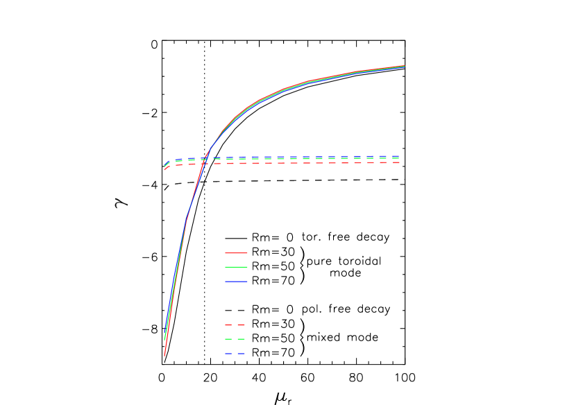
Figure 5: Growth-rates of the $m0$-mode. The dotted vertical line marks the transitional value $\mu_{\rm{r}}^{\rm{t}}\approx 17.5$ at which the pure toroidal mode becomes dominant.

In the free decay case (${\rm{Rm}}=0$) the poloidal (dashed black line) and toroidal (solid black line) modes are decoupled and the growth-rates of these two modes are $\gamma_{m0}=-4.159$ and $\gamma^{\rm{t}}_{m0}=-8.950$, respectively. The decay time of the poloidal eigenmode is significantly larger than that of the toroidal one. The dominant poloidal eigenmode exhibits a typical dipolar pattern as shown in the left panel of figure 6.

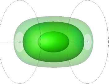
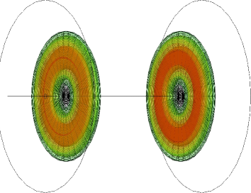
Figure 6: Spatial structure of $m0$-mode in free decay (${\rm{Rm}}=0$). Left panel: $\mu_{\rm{r}}=1$, right panel: $\mu_{\rm{r}}=60$. The isosurfaces show the energy density at 20%, 40%, 80% of the maximum value. The colors code the azimuthal component $H_{\varphi}=\mu_{\rm{r}}^{-1}B_{\varphi}$.

Increasing the disk permeability (still at ${\rm{Rm}}=0$) the poloidal mode remains nearly unaffected (dashed black curve in figure 5) whereas the purely toroidal mode is significantly enhanced and eventually becomes dominant when $\mu_{\rm{r}}\mathrel{\mathchoice{\vbox{\offinterlineskip\halign{\hfil$\displaystyle#$\hfil\cr>\cr\sim\cr}}}{\vbox{\offinterlineskip\halign{\hfil$\textstyle#$\hfil\cr>\cr\sim\cr}}}{\vbox{\offinterlineskip\halign{\hfil$\scriptstyle#$\hfil\cr>\cr\sim\cr}}}{\vbox{\offinterlineskip\halign{\hfil$\scriptscriptstyle#$\hfil\cr>\cr\sim\cr}}}}\mu_{\rm{r}}^{\rm{t}}\approx 17.5$ (see solid curves in figure 5 and right panel in figure 6). The growth-rate of the toroidal mode increases monotonically with $\mu_{\rm{r}}$ and roughly scales $\propto-\mu_{\rm{r}}^{-1}$.

The introduction of a velocity field (${\rm{Rm}}>0$) transfers poloidal field components into toroidal field components, but not vice versa. Therefore for increasing ${\rm{Rm}}$ a mixed mode is generated from the purely poloidal field that is observed at $\rm{Rm}=0$ (see dashed lines in figure 5). The dependence of the growth-rate of the mixed mode with respect to the Reynolds number and the permeability is small. This mixed mode is dominant when $\mu_{\rm{r}}\mathrel{\mathchoice{\vbox{\offinterlineskip\halign{\hfil$\displaystyle#$\hfil\cr<\cr\sim\cr}}}{\vbox{\offinterlineskip\halign{\hfil$\textstyle#$\hfil\cr<\cr\sim\cr}}}{\vbox{\offinterlineskip\halign{\hfil$\scriptstyle#$\hfil\cr<\cr\sim\cr}}}{\vbox{\offinterlineskip\halign{\hfil$\scriptscriptstyle#$\hfil\cr<\cr\sim\cr}}}}\mu_{\rm{r}}^{\rm{t}}$, but above this transitional point it is the purely toroidal eigenmode that dominates (see solid colored curves in figure 5). The purely toroidal mode hardly depends on the magnetic Reynolds number and its growth-rate increases with $\mu_{\rm{r}}$ like in the free decay situation.

Surprisingly, the value of the transitional permeability $\mu_{\rm{r}}^{\rm{t}}$ is more or less the same for all the considered Reynolds numbers (see the vertical dotted line in figure 5 that marks the transition).

4 Discussion on the $m0$-mode

4.1 The coupling

Using the cylindrical coordinate system $(r,{\varphi},z)$, and assuming axisymmetry, the induction equation can be written as follows:

$$\displaystyle\left(\frac{\partial}{\partial t}+u_{r}\frac{\partial}{\partial r}+u_{z}\frac{\partial}{\partial z}\right)B_{r} = \left(\!B_{r}\frac{\partial}{\partial r}\!+\!B_{z}\frac{\partial}{\partial z}\!\right)\!u_{r}+\eta_{0}\!\left[\frac{\partial}{\partial z}\!\left(\frac{\partial}{\partial z}\frac{B_{r}}{\mu_{\rm{r}}}-\frac{\partial}{\partial r}\frac{B_{z}}{\mu_{\rm{r}}}\right)\right],$$ (4)

$$\displaystyle\left[\frac{\partial}{\partial t}+u_{r}\!\left(\frac{\partial}{\partial r}-\frac{1}{r}\right)\!+u_{z}\frac{\partial}{\partial z}\right]\!B_{{\varphi}} = \left[B_{r}\left(\frac{\partial}{\partial r}-\frac{1}{r}\right)+B_{z}\frac{\partial}{\partial z}\right]u_{{\varphi}}+\eta_{0}\Delta_{*}\frac{B_{{\varphi}}}{\mu_{r}},$$ (5)

$$\displaystyle\left(\frac{\partial}{\partial t}+u_{r}\frac{\partial}{\partial r}+u_{z}\frac{\partial}{\partial z}\right)B_{z} = \left(\!B_{r}\frac{\partial}{\partial r}\!+\!B_{z}\frac{\partial}{\partial z}\!\right)u_{z}-\eta_{0}\frac{1}{r}\frac{\partial}{\partial r}\!\left[\!r\!\left(\frac{\partial}{\partial z}\frac{B_{r}}{\mu_{\rm{r}}}-\frac{\partial}{\partial r}\frac{B_{z}}{\mu_{\rm{r}}}\right)\!\right]$$ (6)

where $\Delta_{*}=\frac{\partial^{2}}{\partial r^{2}}+\frac{1}{r}\frac{\partial}{\partial r}+\frac{\partial^{2}}{\partial z^{2}}-\frac{1}{r^{2}}$, and $\eta_{0}=\frac{1}{\sigma\mu_{0}}$. This form of the induction equation clearly shows that $B_{r}=B_{z}=0$ and $B_{\varphi}\neq 0$ can be an axisymmetric solution: this is the purely toroidal mode. If $B_{r}\neq 0,\,B_{z}\neq 0$, then their shearing by the nonzero azimuthal flow $u_{\varphi}$, the so-called $\Omega$-effect, will always generate $B_{\varphi}\neq 0$ which then results in a mixed mode. The growth-rate of the mixed mode will however remain entirely fixed by its poloidal components $B_{r}$ and $B_{z}$ (see figure 5).

Purely toroidal and purely poloidal fields cannot exist if $\mu_{\rm{r}}$ depends on ${\varphi}$. The same remark holds if $\sigma$ depends on ${\varphi}$; for instance, spatial variation of the electric conductivity is used in [1992gafd...64..135B] to produce dynamo action. When the permeability $\mu_{\rm{r}}$ is axisymmetric there is no mechanism to transfer magnetic energy from the toroidal component $B_{\varphi}$ to the poloidal pair $(B_{r},B_{z})$ (see Eqs. 4 and 6).

4.2 Selective enhancement of $B_{\varphi}$

We start by explaining qualitatively why, for large values of $\mu_{\rm{r}}$, the purely toroidal mode is the least damped one and why the mixed mode is so little influenced by the disk. The argument is based on the paramagnetic pumping term (2) that is at the origin of an electromotive force (EMF):

$$\mbox{\boldmath$\mathcal{{E}}$}^{{\mu}}=\mbox{\boldmath$V$}^{\mu}{\times}\mbox{\boldmath$B$}=\frac{1}{\mu_{0}\mu_{\rm{r}}\sigma}\frac{\nabla\mu_{\rm{r}}}{\mu_{\rm{r}}}{\times}\mbox{\boldmath$B$}.$$ (7)

Since the permeability jump is restricted to the material interface there is only a contribution to the EMF within that localized area.

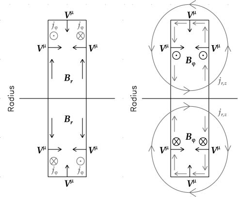
Figure 7: Left panel: current generation at the fluid-disk interface by paramagnetic pumping for a radial magnetic field $B_{r}$. Right panel: current generation from paramagnetic pumping for the azimuthal magnetic field $B_{\varphi}$.

For sufficiently thin disks, as considered here, it is reasonable to assume that the permeability jump at the rim of the impeller disks plays a minor role. We therefore assume that the pumping velocity is mainly axial: $\mbox{\boldmath$V$}^{\mu}\propto\frac{\partial}{\partial z}\mu_{\rm{r}}\mbox{\boldmath$e$}_{z}$. The interaction of $\mbox{\boldmath$V$}^{\mu}$ with the axial field $B_{z}\mbox{\boldmath$e$}_{z}$ is henceforth neglected.

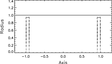
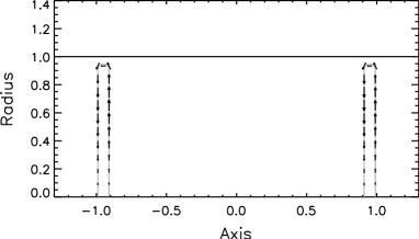
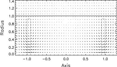
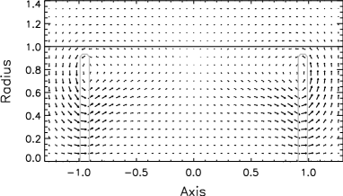
Figure 8: Paramagnetic pumping at $\mu_{\rm{r}}=60$. Upper row: electromotive force (EMF) $\mathcal{E}^{\mu}=({\mu_{0}\mu_{\rm{r}}\sigma})^{-1}\mu_{\rm{r}}^{-1}{\nabla\mu_{\rm{r}}}\times B_{\varphi}\mbox{\boldmath$e$}_{\varphi}$ at ${\rm{Rm}}=0$ (left) and ${\rm{Rm}}=30$ (right). Lower row: (poloidal) current density $\mbox{\boldmath$j$}=({\mu_{0}})^{-1}\nabla\times{\mbox{\boldmath$B$}}/{\mu_{\rm{r}}}$ at ${\rm{Rm}}=0$ (left) and ${\rm{Rm}}=30$ (right). The light grey lines show soft iron disks and the solid horizontal line shows the separation between the moving fluid and stagnant side layer. The azimuthal current is negligible. Note the close similarity between free decay (left column) and the case ${\rm{Rm}}=30$ (right column) illustrating the marginal impact of the fluid flow.

The interaction between $\mbox{\boldmath$V$}^{\mu}\propto\frac{\partial}{\partial z}\mu_{\rm{r}}\mbox{\boldmath$e$}_{z}$ and the radial field $B_{r}\mbox{\boldmath$e$}_{r}$ creates an azimuthal current $j_{\varphi}\mbox{\boldmath$e$}_{\varphi}$ at the interface between the impeller disks and the fluid (see left panel in figure 7). Since the impeller disks are thin, it is reasonable to assume that the orientation and the amplitude of $B_{r}$ do not change across the disks. This implies that the signs of the pumping term (2) at the back and at the front side of the disks are opposite, which in turn implies that the induced azimuthal currents mostly cancel each other and the overall azimuthal current is close to zero. This cancellation mechanism would not occur with thick disks. When the impeller disks are thick, the mixed mode and the purely toroidal mode have similar growth-rates as can be observed in the left panels on figure 8 in 2010GApFD.104..505G 2010GApFD.104..505G where the above phenomenon is illustrated for two thicknesses of the impeller disks, $d=0.1$ and $d=0.6$.

The behavior is very different concerning the EMF that results from the interaction of the azimuthal component $B_{\varphi}\mbox{\boldmath$e$}_{\varphi}$ with $\mbox{\boldmath$V$}^{\mu}$ (see right panel in figure 7). In this case the currents generated at the front and at the back of the impeller disks add up and the EMF drives a poloidal current along the surface of the disk which in turn re-enforces $B_{\varphi}$. Typical patterns of the EMF and current density from our numerical simulations are shown in figure 8. These graphics confirm the presence of the poloidal current and confirm also that the influence of the fluid flow is marginal.

4.3 Simplified model for the toroidal $m0$-mode

Our numerical results clearly indicate that the influence of the flow on the toroidal axisymmetric mode is negligible and that this mode is mostly localized inside the impeller disks. In order to better understand the dynamics of the toroidal $m0$-mode, we consider an idealized disk-fluid model in free decay situation ($\rm{Rm}=0$).

Let us assume a disk of radius $1$, permeability $\mu_{r}\gg 1$ and thickness $d$, sandwiched between two semi-infinite cylindrical fluid regions with $\mu_{\rm{r}}=1$. We further assume the boundary condition $\mbox{\boldmath$H$}{\times}\mbox{\boldmath$n$}=0$ at the wall $r=1$. This simplifying assumption will allow us to find analytical solutions. We solve

$$\mu_{r}\gamma B_{\varphi}=\Delta_{*}\,B_{\varphi},\quad\quad \quad\quad r<1,\quad\quad|z|<d/2$$

$$\ \ \ \gamma B_{\varphi}=\Delta_{*}\,B_{\varphi},\quad\quad \quad\quad r<1,\quad\quad|z|>d/2$$ (8)

where $\Delta_{*}=\frac{\partial^{2}}{\partial r^{2}}+\frac{1}{r}\frac{\partial}{\partial r}+\frac{\partial^{2}}{\partial z^{2}}-\frac{1}{r^{2}}$. Note that the non-dimensionalization is done so that the reference scale of the growth-rate is $(\sigma\mu_{0}R^{2})^{-1}$. The boundary condition is $B_{\varphi}=0$ at $r=1$, and the transmission condition across the material interface is that $H_{\varphi}$ and $E_{r}=\partial_{z}H_{\varphi}/\sigma$ be continuous at $z=\pm d/2$.

The numerical simulations show that the dominating eigenmodes are symmetric with respect to the equatorial plane of the disk $z=0$. This leads to the following ansatz

$$B_{\varphi} = A_{1}\,J_{1}(kr)\,\cos l_{1}z,\ \quad\quad r<1,\quad\quad 0<z<d/2$$

$$B_{\varphi} = A_{2}\,J_{1}(kr)\,e^{-L_{2}z},\quad\quad\quad r<1,\quad\quad z>d/2,$$

where $J_{1}$ is the Bessel function of the first kind and

$$l_{1}=\sqrt{-\gamma\mu_{r}-k^{2}},\quad\quad L_{2}=\sqrt{k^{2}+\gamma}.$$ (9)

The amplitudes $A_{1}$ and $A_{2}$ are arbitrary for the moment. The fields are obtained by symmetry for $z<0$. To ensure that the solution decays at infinity (i.e. it remains bounded when $z\to\pm\infty$), it is necessary that $l_{1}$ and $L_{2}$ be real. This imposes the constraints

$$\mu_{r}>1\quad,\quad\gamma\in[-k^{2},-k^{2}/\mu_{r}].$$ (10)

The boundary condition at $r=1$ implies that $J_{1}(k)=0$, i.e. $k$ is a zero of $J_{1}$. We choose the first zero, say $k_{1}$, so that the solution is composed of one radial cell only,

$$k_{1}\approx 3.8317.$$ (11)

This value specifically depends on the idealized boundary condition that we have assumed at $r=1$; the effect of small deviations $k=(1\pm 0.1)k_{1}$ is considered further below. Due to the assumed symmetry, we need to impose the transmission conditions at the $z=d/2$ interface only:

$$\ \left(\frac{1}{\mu_{r}}\ \cos\frac{l_{1}d}{2}\right)A_{1}-\left(e^{-L_{2}d/2}\right)A_{2} = 0,$$

$$\left(\frac{l_{1}}{\sigma\mu_{r}}\,\sin\frac{l_{1}d}{2}\right)A_{1}-\left(\frac{L_{2}}{\sigma}\,e^{-L_{2}d/2}\right)A_{2} = 0.$$ (12)

The determinant of the above linear system must be zero for a solution to exist,

$$L_{2}\cos\frac{l_{1}d}{2}-l_{1}\sin\frac{l_{1}d}{2}=0.$$ (13)

Upon inserting the definitions of $l_{1}$ and $L_{2}$ from (9) into this dispersion relation, we obtain an implicit nonlinear equation for the growth-rate $\gamma$ as a function of $d$ and $\mu_{\rm{r}}$.

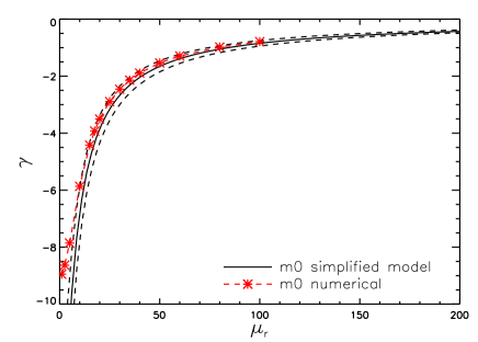
Figure 9: (left) Growth-rate $\gamma$ as a function of $\mu_{r}$ for the dominant axisymmetric toroidal eigenmode from the simplified model. $d=0.1$, $k=k_{1}$ and $k=(1\pm 0.1)k_{1}$. (right) Using the proper time scale $\sigma\mu_{r}\mu_{0}R^{2}$ involving the permeability of the impeller disk, the growth-rate $\tilde{\gamma}=\gamma\mu_{r}$ reaches an asymptote at high $\mu_{r}$.

We show in the left panel of figure 9 the graph of the function $\gamma(\mu_{\rm{r}})$ deduced from (13) with $d=0.1$ and $k=k_{1}=3.8317$. Two further analytical graphs computed with $k=(1\pm 0.1)k_{1}$ show the very weak sensitivity of the growth rate on relaxing the strict boundary condition $\mbox{\boldmath$H$}\times\mbox{\boldmath$n$}=0$ (e.g. by using an outer shell of different conductivity). We also show in this figure the numerical outcome for the growth-rate of the purely toroidal mode at $\rm{Rm}=0$ (see also black solid line in figure 5). The agreement is quite satisfactory and thereby confirms our analysis. When representing $\gamma(\mu_{\rm{r}})$ in $\log$-$\log$ scale (not shown) we see that $\gamma(\mu_{\rm{r}})$ scales like $\mu_{r}^{-1}$ in the limit $\mu_{r}\rightarrow\infty$. Actually this behavior depends on the choice that we have made for the non-dimensionalization. Involving the disks permeability for defining the new timescale $(\sigma\mu_{r}\mu_{0}R^{2})$ instead of $(\sigma\mu_{0}R^{2})$, we obtain the rescaled growth-rate $\tilde{\gamma}=\gamma\mu_{r}$ shown in the right-panel of figure 9. This representation shows that the growth-rate $\tilde{\gamma}$ reaches a constant value for very high permeabilities ($\tilde{\gamma}_{\infty}=-86.6631$). This observation immediately implies that the following power law $\gamma\sim\tilde{\gamma}_{\infty}/\mu_{\rm{r}}$ holds in the original units when $\mu_{\rm{r}}\to+\infty$.

In conclusion, the above simplified model explains why the growth-rate of the purely toroidal mode goes to zero when $\mu_{r}\rightarrow\infty$. The model shows also that although the dominant purely toroidal mode is localized to a very small volume, its decay time determines the overall decay of the axisymmetric azimuthal magnetic field. Note finally that this mode would not be observed in numerical simulations of VKS-dynamos that use the idealized boundary condition $\mbox{\boldmath$H$}{\times}\mbox{\boldmath$n$}=0$ on the disk’s surface (see e.g. 2008giss).

5 Conclusions

The aim of this paper is to study the influence of thin high permeability disks on a VKS-like dynamo model. This work goes well beyond the study of 2010GApFD.104..505G in the sense that we investigate thoroughly the axisymmetric mode and present novel details on the scaling behavior of the dynamo $m1$-mode. The high permeability disks facilitate the occurrence of non-axisymmetric dynamo action by enhancing the growth-rate of the equatorial dynamo $m1$-mode. Compared to the idealized limit ($\mu_{r}\rightarrow\infty$) the presence of a finite but high permeability material adds a small supplementary damping effect and therefore slightly increases the dynamo threshold. We propose that the observed $\mu_{r}^{-1/2}$-scaling for the dynamo threshold can be explained by a skin-effect so that that the disk’s role on the $m1$-mode is quite passive. Although the reduction of the magnetic Reynolds number is substantial (from ${\rm{Rm}}^{\rm{c}}\approx 76$ at $\mu_{\rm{r}}=1$ to ${\rm{Rm}}^{\rm{c}}\approx 54$ in the limit $\mu_{\rm{r}}\rightarrow\infty$) the spatial structure of the $m1$-mode is hardly changed.

The effects of the high permeability of the impeller disks on the axisymmetric mode turn out to be more fundamental. In the presence of a mean flow the axisymmetric $m0$-modes are split up in two separate families, one consisting of a purely toroidal mode and one consisting of a mixed mode composed of a poloidal and a toroidal component. The growth-rate of the mixed $m0$-mode slightly increases with $\rm{Rm}$ but is nearly independent of the disk permeability. The growth-rate of the purely toroidal $m0$-mode is not significantly influenced by the flow amplitude, but it is considerably enhanced $\propto\mu_{\rm{r}}^{-1}$ for large values of $\mu_{r}$. This selective enhancement of the purely toroidal $m0$-mode can be explained qualitatively by paramagnetic pumping. A simplified analytical model that interprets the purely toroidal mode as a localized free decay solution confirms the scaling obtained in the numerical simulations. This slowly decaying purely toroidal mode promoted through the high permeability disks may play an important role in axisymmetric dynamo action. However, in our simple axisymmetric set-up no possibility for a closure of the dynamo cycle is provided since the poloidal component remains decoupled from the dominant toroidal field so that such dynamo remains impossible [1933MNRAS..94...39C, 1982GApFD..19..301H].

Our study shows that the ideal boundary conditions $\mbox{\boldmath$H$}\times\mbox{\boldmath$n$}=0$ is indeed a reasonable assumption for the $m1$-mode, but it is not appropriate for the analysis of the toroidal $m0$-mode. The purely toroidal $m0$-mode can be obtained only by explicitly considering the internal permeability distribution and the corresponding jump conditions at the fluid/disk interface. This mode cannot be obtained numerically by simulations of VKS-like dynamos that use either the idealized boundary condition $\mbox{\boldmath$H$}{\times}\mbox{\boldmath$n$}=0$ at the fluid/disk interface or the thin-wall approximation from 2010GApFD.104..207R.

In conclusion, we have seen that the high (but finite) permeability in the impeller disks is very important to promote axisymmetric modes in our model and we suppose that it may also play a nontrivial role in the real VKS experiment. For example, in the presence of more complex (non-axisymmetric) flows containing small scale turbulence modeled by an $\alpha$-effect [2008PhRvL.101j4501L, andregafd], or in the presence of non-axisymmetric permeability distributions that resemble the soft-iron blades attached to the disks [PhysRevLett.104.044503], the purely toroidal $m0$-modes can be coupled with poloidal field components thus providing the required mechanism to close the dynamo loop.

References

References

- [1] \harvarditemBusse \harvardand Wicht19921992gafd…64..135B Busse F H \harvardand Wicht J 1992 Geophys. Astrophys. Fluid Dyn. 64, 135–144.
- [2] \harvarditemCowling19331933MNRAS..94…39C Cowling T G 1933 Mon. Not. R. Astr. Soc. 94, 39–48.
- [3] \harvarditemDobler et al.20032003PhRvE..67e6309D Dobler W, Frick P \harvardand Stepanov R 2003 Phys. rev. E 67(5), 056309.
- [4] \harvarditemDudley \harvardand James19891989RSPSA.425..407D Dudley M L \harvardand James R W 1989 Proc. R. Soc. Lond. A 425, 407–429.
- [5] \harvarditemGiesecke et al.20082008giesecke_maghyd Giesecke A, Stefani F \harvardand Gerbeth G 2008 Magnetohydrodynamics 44(3), 237–252.
- [6] \harvarditemGiesecke et al.2010aandregafd Giesecke A, Nore C, Plunian F, Laguerre R, Ribeiro A, Stefani F, Gerbeth G, Leorat J \harvardand Guermond J 2010a Geophys. Astrophys. Fluid Dyn. 104(2), 249–271.
- [7] \harvarditemGiesecke et al.2010bPhysRevLett.104.044503 Giesecke A, Stefani F \harvardand Gerbeth G 2010b Phys. Rev. Lett. 104(4), 044503.
- [8] \harvarditemGiesecke et al.2010c2010GApFD.104..505G Giesecke A, Nore C, Stefani F, Gerbeth G, Leorat J, Luddens F \harvardand Guermond J 2010c Geophys. Astrophys. Fluid Dyn. 104, 505–529.
- [9] \harvarditemGissinger et al.20082008giss Gissinger C, Iskakov A, Fauve S \harvardand Dormy E 2008 Europhys. Lett. 82, 29001.
- [10] \harvarditemGuermond et al.2007guermond2007 Guermond J L, Laguerre R, Léorat J \harvardand Nore C 2007 J. Comp. Phys. 221(1), 349–369.
- [11] \harvarditemGuermond et al.2011GLLNR11 Guermond J L, Léorat J, Luddens F, Nore C \harvardand Ribeiro A 2011 J. Comp. Phys. 230, 6299–6319.
- [12] \harvarditemHide \harvardand Palmer19821982GApFD..19..301H Hide R \harvardand Palmer T N 1982 Geophys. Astrophys. Fluid Dyn. 19, 301–309.
- [13] \harvarditemIskakov et al.2004iskakov2004 Iskakov A B, Descombes S \harvardand Dormy E 2004 J. Comp. Phys. 197(2), 540–554.
- [14] \harvarditemKrause \harvardand Rädler19801980mfmd.book…..K Krause F \harvardand Rädler K H 1980 Mean-field magnetohydrodynamics and dynamo theory Oxford: Pergamon Press.
- [15] \harvarditemLaguerre et al.20082008PhRvL.101j4501L Laguerre R, Nore C, Ribeiro A, Léorat J, Guermond J \harvardand Plunian F 2008 Phys. Rev. Lett. 101(10), 104501.
- [16] \harvarditemLowes \harvardand Wilkinson19631963Natur.198.1158L Lowes F J \harvardand Wilkinson I 1963 Nature 198, 1158–1160.
- [17] \harvarditemLowes \harvardand Wilkinson19681968Natur.219..717L Lowes F J \harvardand Wilkinson I 1968 Nature 219, 717–718.
- [18] \harvarditemMarié et al.20062004phfl Marié L, Normand C \harvardand Daviaud F 2006 Phys. Fluids 18, 017102.
- [19] \harvarditemMonchaux et al.20072007PhRvL..98d4502M Monchaux R, Berhanu M, Bourgoin M, Moulin M, Odier P, Pinton J F, Volk R, Fauve S, Mordant N \harvardand Pétrélis F 2007 Phys. Rev. Lett. 98(4), 044502.
- [20] \harvarditemMonchaux et al.20092009PhFl…21c5108M Monchaux R, Berhanu M, Aumaître S, Chiffaudel A, Daviaud F, Dubrulle B, Ravelet F, Fauve S, Mordant N, Pétrélis F, Bourgoin M, Odier P, Pinton J F, Plihon N \harvardand Volk R 2009 Phys. Fluids 21(3), 035108.
- [21] \harvarditemRavelet et al.2005ravelet2005 Ravelet F, Chiffaudel A, Léorat J \harvardand Daviaud F 2005 Phys. Fluids 17, 117104.
- [22] \harvarditemRoberts et al.20102010GApFD.104..207R Roberts P H, Glatzmaier G A \harvardand Clune T L 2010 Geophys. Astrophys. Fluid Dyn. 104, 207–220.
- [23] \harvarditemStefani et al.20062005physics..11149S Stefani F, Xu M, Gerbeth G, Ravelet F, Chiffaudel A, Daviaud F \harvardandLéorat J, 2006 Eur. J. Mech. B 25, 894–908.
- [24] \harvarditemVerhille et al.20102010NJPh…12c3006V Verhille G, Plihon N, Bourgoin M, Odier P \harvardand Pinton J 2010 New J. Phys. 12(3), 033006.
- [25] \harvarditemWicht \harvardand Busse19931993spd..conf..329W Wicht J \harvardand Busse F H 1993 in M. R. E. Proctor, P. C. Matthews, & A. M. Rucklidge, ed., ‘Solar and Planetary Dynamos’ pp. 329–337.
- [26]