Combined Base Station Association and Power Control in Multi-channel Cellular Networks

Abstract

A combined base station association and power control problem is studied for the uplink of multichannel multicell cellular networks, in which each channel is used by exactly one cell (i.e., base station). A distributed association and power update algorithm is proposed and shown to converge to a Nash equilibrium of a noncooperative game. We consider network models with discrete mobiles (yielding an atomic congestion game), as well as a continuum of mobiles (yielding a population game). We find that the equilibria need not be Pareto efficient, nor need they be system optimal. To address the lack of system optimality, we propose pricing mechanisms. It is shown that these mechanisms can be implemented in a distributed fashion.

I Introduction

Wireless communication systems have experienced tremendous growth over the last decade, and this growth continues unabated worldwide. Efficient management of resources is essential for the success of wireless cellular systems. In a mobile cellular system, mobiles adapt to time varying radio channels by adjusting base station (BS) associations and by controlling transmitter powers. Doing so, they not only maintain their quality of service (QoS) but also enhance their transmitters’ battery lives. In addition, such controls reduce the network interference, thus maximizing spatial spectrum reuse. Distributed control is of special interest, since the alternative of centrally orchestrated control involves added infrastructure, the need for distribution of measurements, and hence system complexity.

Distributed control algorithms for single channel multicell networks have been extensively studied (Foschini & Miljanic [1], Yates [2], Hanly [3]). The monograph by Chiang et al. [4] and references therein provide an excellent survey of the area. Noncooperative games have been a natural tool for analysis and design of distributed power control algorithms. Scutari et al. [5] and Heikkinen [6] model distributed power control problems as potential games, while Altman & Altman [7] show that many of the cellular power control algorithms can be modeled as submodular games. In contrast, uplink resource allocation for multichannel multicell networks poses several challenges as observed in Yates [2] and Jiang et al. [8].

We address the resource allocation problem in the uplink of a multichannel multicell network with a single traffic class. Such a problem arises when a CDMA operator chooses to lease and utilize multiple frequency bands in order to reduce in-network interference, or multiple operators who lease different bands decide to cooperate. The newer mobile devices are typically radio agile, and thus have the option to choose from one of these distinct bands. We address a simplified version of this multichannel multicell problem where all BSs operate on different frequency bands.

A preview of our results is as follows. We propose a distributed algorithm for the combined base station association and power control problem, and subsequently model the problem as a player-specific congestion game. The equilibrium states of such algorithms, which are Nash equilibria of the corresponding games, may be far from system optimum. We resort to pricing mechanisms to induce mobiles to behave in a way that optimizes system cost. We also show that such a mechanism can be employed in a distributed fashion. Towards this end, we model the network as having a continuum of (nonatomic) mobiles, each offering infinitesimal load, which leads to a population game formulation. We then provide a marginal pricing mechanism that motivates a pricing strategy for the discrete mobiles case. Note that, unlike the case of transportation networks, mobiles are not really priced in cellular networks. The pricing is simply a part of the decision making routine built into each mobile in order bring about a distributed control mechanism that drives the system toward optimality.

The paper is organized as follows. In Section II we briefly discuss concepts of finite noncooperative games and population games. We study a network model with discrete mobiles in Section III. We propose a combined association and power control algorithm, model it as a noncooperative game, and analyze its performance. We extend this analysis to a network with a continuum of mobiles in Section IV. To address the inefficiency of the proposed algorithms, we design toll mechanisms in Section V. Finally, we conclude the paper with some remarks in Section VI.

Optimal power allocation and BS association in uplinks of multichannel multicell cellular networks have not been explored before. Ours is an attempt at a detailed coverage on what is possible in general, with more specific results in some special cases.

II Game Preliminaries

II-A Finite Noncooperative Games

A noncooperative strategic form game $(\mathcal{M},(\mathcal{A}_{i},i\in\mathcal{M}),(c_{i},i\in\mathcal{M}))$ consists of a set of players $\mathcal{M}=\{1,\dots,M\}$. Each player $i$ is accompanied by an action set $\mathcal{A}_{i}$ and a cost function $c_{i}:\times_{i=1}^{M}\mathcal{A}_{i}\rightarrow\mathbb{R}$. In this work, we assume all action sets to be finite. An action profile $\mathbf{a}=(a_{i},i=1,\dots,M)$ prescribes an action $a_{i}$ for every player $i\in\mathcal{M}$. For $\mathbf{a}=(a_{i},i=1,\dots,M)$, denote $\mathbf{a}_{-i}:=(a_{1},\dots,a_{i-1},a_{i+1},\dots,a_{M})$ and $(b_{i},\mathbf{a}_{-i}):=(a_{1},\dots,a_{i-1},b_{i},a_{i+1},\dots,a_{M})$.

Definition II.1

Nash Equilibrium (NE): For an action profile $\mathbf{a}$, a mobile $i$’s best response, $\mathcal{B}_{i}(\mathbf{a})\subseteq\mathcal{A}_{i}$, is defined as $\mathcal{B}_{i}(\mathbf{a}):=\operatornamewithlimits{argmin}_{b_{i}\in\mathcal{A}_{i}}c_{i}(b_{i},a_{-i})$. $\mathbf{a}$ is said to be a Nash Equilibrium for the game if $a_{i}\in\mathcal{B}_{i}(\mathbf{a})$ for all $i\in\mathcal{M}$.

Definition II.2

Potential Game: A game $(\mathcal{M},(\mathcal{A}_{i},i\in\mathcal{M}),(c_{i},i\in\mathcal{M}))$ is said to be an ordinal potential game if there exists a function $V:\times_{i=1}^{M}\mathcal{A}_{i}\rightarrow\mathbb{R}$, known as an ordinal potential function, that satisfies

$$c_{i}(b_{i},\mathbf{a}_{-i})<c_{i}(\mathbf{a})\Leftrightarrow V(b_{i},\mathbf{a}_{-i})<V(\mathbf{a})$$

for all $i\in\mathcal{M},b_{i}\in\mathcal{A}_{i},\mathbf{a}\in\times_{i=1}^{M}\mathcal{A}_{i}$.

Clearly, all minimizers of an ordinal potential function $V$ are Nash equilibria of the game. Thus all ordinal potential games $(\mathcal{M},(\mathcal{A}_{i},i\in\mathcal{M}),(c_{i},i\in\mathcal{M}))$ admit at least one Nash equilibrium. On account of their finiteness they also have the finite improvement path (FIP) property, i.e., do not contain improvement cycles (Monderer & Shapley [9, Lemma 2.3]). Thus, in a finite ordinal potential game when players update as per the better response strategy, round-robin or random update processes converge to a Nash equilibrium in a finite number of steps. With the same strategies, an asynchronous update process also converges (Neel [10, Chapter 5]).

Remark II.1

The strategic form games that have the FIP property also admit the finite best-response path (FBRP) property, i.e., do not contain best response cycles (Milchtaich [11, Section 5]). Thus, if players update as per the best response strategy, then also the above update processes converge to a Nash equilibrium in a finite number of steps. The reverse implication is not true in general - FBRP need not imply FIP.

Definition II.3

Congestion Game: A game $(\mathcal{M},(\mathcal{A}_{i},i\in\mathcal{M}),(c_{i},i\in\mathcal{M}))$ is said to be a player-specific weighted singleton congestion game if

1. there exists a set $\mathcal{N}$ such that $\mathcal{A}_{i}=\mathcal{N}$ for all $i\in\mathcal{M}$, and

2. there exist constants $(\beta_{i},i\in\mathcal{M})$ and nonincreasing functions $f_{ij},i\in\mathcal{M},j\in\mathcal{N}$ such that

   $$c_{i}(\mathbf{a})=f_{ia_{i}}(\sum_{\stackrel{{\scriptstyle l\in\mathcal{M}:}}{{a_{l}=a_{i}}}}\beta_{l})\mbox{ for all }\mathbf{a}\in\times_{i=1}^{M}\mathcal{A}_{i},i\in\mathcal{M}.$$

In the above definition, we interpret $\mathcal{N}$ as a set of facilities and $\beta_{l}$ as the load offered by player $i$. Then, $\sum_{\stackrel{{\scriptstyle l\in\mathcal{M}:}}{{a_{l}=a_{i}}}}\beta_{l}$ denotes the total load on facility $a_{i}$, under an action profile $\mathbf{a}$. The game is a singleton congestion game because each action picks exactly one facility. It is weighted because players offer different loads, and it is player-specific because the cost functions $c_{i}(\cdot)$ are player-specific.

Rosenthal [13] has defined congestion games with unweighted players and player-independent cost functions, but more general action sets. The above generalization is due to Milchtaich [11] who also showed that singleton congestion games with weighted players but player independent costs admit FIP. Gairing et al. [14] studied these games in the special case of linear cost functions. Georgiou et al. [15] introduced a routing game where the players only have incomplete information about edge latencies, and showed that this game can be transformed into a (complete information) player specific singleton congestion game with linear cost functions. Mavronicolas et al. [16] considered a subclass where each player-specific cost function is composed (by means of an abelian group operation) of a player-specific constant and a facility-specific nondecreasing function.

II-B Population Games

A population game (Sandholm [17]) $(\mathcal{M},(\mathcal{A}_{l},l\in\mathcal{L}),(c_{lj},l\in\mathcal{L},j\in\mathcal{A}_{l}))$ consists of $\mathcal{L}=\{1,\dots,L\}$ classes of nonatomic populations of players. $\mathcal{M}=\cup_{l\in\mathcal{L}}\mathcal{M}_{l}$, and $M_{l}:=|\mathcal{M}_{l}|$ denotes the total mass of the class $l$ population. By a nonatomic population, we mean that the mass of each member of the population is infinitesimal. Players of class $l$ are associated with an action set $\mathcal{A}_{l}$. Actions of these (class $l$) players lead to an action distribution $\mathbf{m}^{l}=(m_{lj},j\in\mathcal{A}_{l})$, where $\sum_{j\in\mathcal{A}_{l}}m_{lj}=M_{l}$. All the players within a class are alike. Thus the action distributions completely specify the play; we can characterize the states and dynamics of play solely in terms of action distributions. Let $\mathbf{m}=(\mathbf{m}^{l},l\in\mathcal{L})$ denote the action distribution profile across the entire population, and let $\mathcal{M}^{\ast}$ denote the set of all such profiles. A population $l$ is also accompanied by continuous cost density functions $c_{lj}:\mathcal{M}^{\ast}\rightarrow\mathbb{R}$.

Definition II.4

Nash Equilibrium (NE): An action distribution profile $\mathbf{m}$ is a pure strategy Nash equilibrium for the game $(\mathcal{M},(\mathcal{A}_{i},i\in\mathcal{M}),(c_{lj},l\in\mathcal{L},j\in(\mathcal{A}_{l}))$ if and only if for all $l\in\mathcal{L}$ and $j\in\mathcal{A}_{l}$, a positive mass $m_{lj}>0$ implies $c_{lj}(\mathbf{m})\leq c_{lk}(\mathbf{m})$ for all $k\in\mathcal{A}_{l}$.

Remark II.2

At a Nash equilibrium $\mathbf{m}$, for a class $l$, if $j$ and $k$ are any two facilities in $\mathcal{A}_{l}$ such that $m_{lj}>0,m_{lk}>0$, then $c_{lj}(\mathbf{m})=c_{lk}(\mathbf{m})$.

Definition II.5

Potential Game: A game $(\mathcal{M},(\mathcal{A}_{l},l\in\mathcal{L}),(c_{lj},l\in\mathcal{L},j\in\mathcal{A}_{l}))$ is said to be a potential game if there exists a $\mathbf{C}^{1}$ function $V:\mathcal{M}^{\ast}\rightarrow\mathbb{R}$, known as a potential function, that satisfies

$$\frac{\partial V(\mathbf{m})}{\partial m_{lj}}=c_{lj}(\mathbf{m})$$

for all $l\in\mathcal{L},j\in\mathcal{A}_{l},\mathbf{m}\in\mathcal{M}^{\ast}$.

It is well known that Nash equilibria are the profiles which satisfy the Kuhn-Tucker first order conditions for a minimizer of the potential function (Sandholm [17, Proposition 3.1]). Any dynamics with positive correlation and noncomplacency (in particular the best response dynamics) approaches a Nash equilibrium [17].

We are interested in nonatomic congestion games (Sandholm [17]), in which $\mathcal{A}_{l}=\mathcal{N},\forall l\in\mathcal{L}$, for a given set $\mathcal{N}$. As before, we interpret $\mathcal{N}$ as a set of facilities. Moreover, each class $l$ has an associated offered load density $\gamma_{l}>0$. An action distribution profile $\mathbf{m}$ leads to a congestion profile $(m_{j},j\in\mathcal{N})$, where $m_{j}=\sum_{l\in\mathcal{L}}m_{lj}\gamma_{l}$. The cost density functions $c_{lj}$ depend on $\mathbf{m}$ only through $m_{j}$, and are increasing in $m_{j}$.

II-C Pricing

Levying of tolls is a conventional way to enforce system optimality in nonatomic networks. Beckman [18] and Dafermos & Sparrow [19] studied optimal tolls in transportation networks with a single class of users. Later Dafermos [20] and Smith [21] extended the analysis to multiclass networks. Roughgarden & Tardos [22] applied these ideas in computer networks and analyzed tolls for optimal routing.

In the atomic (discrete) setting, Caragiannis et al. [23] proposed tolls for two-terminal parallel-edge networks with unweighted users and linear latency functions. Fotakis & Spirakis [24] extended these to generic two-terminal networks with unweighted users and arbitrary increasing latency functions. We propose an alternative toll mechanism, and demonstrate that the proposed tolls can be computed in a distributed fashion.

III Discrete Mobiles

III-A System Model

We now describe the model adopted in this work. We consider the uplink of a cellular network consisting of several BSs and mobiles. Each BS operates in a distinct frequency band. Let $\mathcal{N}=\{1,\dots,N\}$ and $\mathcal{M}=\{1,\dots,M\}$ denote the set of BSs and the set of mobiles, respectively.

A mobile must be associated with one BS at any time, and is free to choose the BS with which it associates. Let $h_{ij}$ denote the power gain from mobile $i$ to BS $j$. Let the receiver noise at all BSs have the average power $\sigma^{2}$. Let $p_{i}$ denote the power transmitted by mobile $i$, and let $a_{i}$ be the BS to which it is associated. Under an association profile $\mathbf{a}=(a_{i},i=1,\dots,M)$, let $\mathcal{M}_{j}(\mathbf{a})$ be the set of mobiles associated with BS $j$. Under an association profile $\mathbf{a}=(a_{i},i=1,\dots,M)$ and a power vector $\mathbf{p}=(p_{i},i=1,\dots,M)$, the signal to interference plus noise ratio (SINR) of mobile $i$ at BS $a_{i}$ is

$$\frac{h_{ia_{i}}p_{i}}{\sum_{l\in\mathcal{M}_{a_{i}}(\mathbf{a})\setminus\{i\}}h_{la_{l}}p_{l}+\sigma^{2}}$$

Mobile $i$ has a target SINR requirement $\gamma_{i}$.

III-B The Proposed Algorithm

Yates [2] and Hanly [3] proposed an algorithm for distributed association and power control in single channel cellular networks. Convergence results for the algorithm are based on the concept of a standard interference function. The technique is based on a mobile reassociating itself with a BS with which it needs to use the least power; this fails to work in the case of a multichannel network and analogous convergence results for this algorithm may not hold (see Yates [2, Section VI]). Even in instances where the algorithm converges, it may get stuck at a power allocation that is not Pareto efficient.

We propose an alternative distributed algorithm for combined BS association and power control in multichannel multicell cellular networks. We also show its convergence. We make use of the following simple fact (see, for example, Kumar et al. [25, Chapter 5]). Consider the subproblem of power control with a fixed association $\mathbf{a}$. Define $\beta_{l}=\frac{\gamma_{l}}{1+\gamma_{l}}$, a measure of the “load” offered by mobile $l$.

Proposition III.1

For a fixed association $\mathbf{a}$,
(i) The power control subproblem of BS $j$ is feasible iff $\sum_{l\in\mathcal{M}_{j}(\mathbf{a})}\beta_{l}<1$.
(ii) If the power control subproblem of BS $j$ is feasible, there exists a unique Pareto efficient power vector $\mathbf{p}(\mathbf{a})$ given by

$$p_{i}(\mathbf{a})=\frac{\sigma^{2}}{h_{ij}}\frac{\beta_{i}}{1-\sum_{l\in\mathcal{M}_{j}(\mathbf{a})}\beta_{l}}.$$

Throughout we assume that there exists at least one feasible association and power vector. Proposition III.1 motivates the following algorithm.

Multichannel Association and Power Control (MAPC): Mobiles switch associations in a round-robin fashion by taking into account the optimal power consumptions (given by Proposition III.1(ii)) at the BSs with which these associate. This is done as follows. As the load at a BS changes, it immediately broadcasts the new load, and associated mobiles update their powers to the optimal required powers as per the new loads. To be more precise, define

$$c_{i}(\mathbf{a})=\frac{\sigma^{2}}{h_{ia_{i}}}\frac{\beta}{[1-\sum_{l\in\mathcal{M}_{j}(\mathbf{a})}\beta_{l}]^{+}},$$ (1)

where $[x]^{+}=\max(x,0)$. For $t=0,1,2,\dots$, mobile $i$ where $i=1+(t\mod M)$ updates its association and power at $t+1$ if $a_{i}(t)\notin\operatornamewithlimits{argmin}_{j\in\mathcal{N}}c_{i}((j,\mathbf{a}(t)_{-i}))$. In this case,

$$a_{i}(t+1)\in\operatornamewithlimits{argmin}_{j\in\mathcal{N}}c_{i}((j,\mathbf{a}(t)_{-i})),$$ (2a)

$$\mbox{and with }\mathbf{a}(t+1)=(a_{i}(t+1),\mathbf{a}(t)_{-i}),$$

$$p_{l}(t+1)=c_{l}(\mathbf{a}(t+1)),$$

$$\ \ \ \ \ \ \forall l\in\mathcal{M}_{a_{i}(t)}(\mathbf{a}(t))\cup\mathcal{M}_{a_{i}(t+1)}(\mathbf{a}(t+1)).$$ (2b)

Remark III.1

A mobile $i$ should not choose a BS if the device renders the corresponding power control subproblem infeasible. The situation is characterized by $\sum_{l\in\mathcal{M}_{j}(\mathbf{a})}\beta_{l}\geq 1$, and (1) appropriately yields infinite cost for the mobile. Even if the algorithm starts with an infeasible association, selfish moves of players eventually lead to a feasible one, and updates remain feasible thereafter.

Note that while only one mobile updates its association at a time, all mobiles that perceive a change in load at their BSs update their powers to optimal values based on the new loads. Simultaneous association updates are not allowed. In a framework with no synchronizing agent and with an arbitrarily fine time-scale, it is unlikely that two mobiles update simultaneously. If two or more BSs result in the same steady state power, one is chosen at random by the mobile.

This algorithm is also distributed in nature as the one proposed in Yates [2]. BS $j$ broadcasts its total congestion $\sum_{l\in\mathcal{M}_{j}(\mathbf{a})}\beta_{l}$. In addition, each mobile $i$ is told its scaled gains $\frac{h_{ij}}{\sigma^{2}}$ by each BS $j\in\mathcal{N}$.

III-C A Congestion Game Formulation

To show the convergence properties of the proposed algorithm, we model the system as a strategic form game. Let the mobiles be the players and the action set for each player be the possible associations, i.e, $\mathcal{A}_{i}=\mathcal{N}$ for all $i\in\mathcal{M}$. Define the cost functions of the players to be $c_{i}(\mathbf{a})$ for all $i\in\mathcal{M}$. It can be seen that above is a player-specific singleton weighted congestion game, and belongs to the subclass of congestion games with multiplicative player-specific constants described in [16]. In the following we refer to it as the strategic form game $(\mathcal{M},\mathcal{N},(c_{i},i\in\mathcal{M}))$.

Before analyzing the general game, we consider the following special cases.

III-C1 Single Class Traffic

This is the case where all the mobiles have a common target SINR requirement $\gamma$; $\beta:=\frac{\gamma}{1+\gamma}$. In this case,

$$c_{i}(\mathbf{a})=\frac{\sigma^{2}}{h_{ia_{i}}}\frac{\beta}{[1-|\mathcal{M}_{a_{i}}(\mathbf{a})|\beta]^{+}}$$

and we have a player specific unweighted singleton congestion game.

III-C2 Collocated Users

In this case, all mobiles are situated close together in a group. Thus $h_{ij}=h_{j}$ for all $i\in\mathcal{M},j\in\mathcal{N}$, and

$$c_{i}(\mathbf{a})=\frac{\sigma^{2}}{h_{a_{i}}}\frac{\beta_{i}}{[1-\sum_{l\in\mathcal{M}_{a_{i}}(\mathbf{a})}\beta_{l}]^{+}}.$$

This yields a player independent weighted singleton congestion game.

III-C3 Collocated BS

Here all BSs are assumed to be situated close together. Thus $h_{ij}=h_{i}$ for all $i\in\mathcal{M},j\in\mathcal{N}$, and

$$c_{i}(\mathbf{a})=\frac{\sigma^{2}}{h_{i}}\frac{\beta_{i}}{[1-\sum_{l\in\mathcal{M}_{a_{i}}(\mathbf{a})}\beta_{l}]^{+}}.$$

Now, we get a player specific weighted singleton congestion game.

The following result ensures that MAPC converges in each of these special cases.

Proposition III.2

The finite strategic form game $(\mathcal{M},\mathcal{N},(c_{i},i\in\mathcal{M}))$ is an ordinal potential game and thus admits the FIP in each of the following cases.

1. $\beta_{i}=\beta$ for all $i\in\mathcal{M}$,

2. $h_{ij}=h_{j}$ for all $i\in\mathcal{M},j\in\mathcal{N}$,

3. $h_{ij}=h_{i}$ for all $i\in\mathcal{M},j\in\mathcal{N}$.

Proof:

In each case, we show that the game $(\mathcal{M},\mathcal{N},(c_{i},i\in\mathcal{M}))$ is better response equivalent (Neel [10, Chapter 5]) to an ordinal potential game (by demonstrating an ordinal potential function for the latter). This implies that, in each case, $(\mathcal{M},\mathcal{N},(c_{i},i\in\mathcal{M}))$ itself is an ordinal potential game. It is also finite which implies that the FIP property holds.
$1)$ The strategic form game $(\mathcal{M},\mathcal{N},(c_{i},i\in\mathcal{M}))$ is better response equivalent to $(\mathcal{M},\mathcal{N},(-\frac{1}{c_{i}},i\in\mathcal{M}))$. Also note that

$$-\frac{1}{c_{i}(\mathbf{a})}=-\frac{h_{ia_{i}}}{\sigma^{2}}\frac{[1-|\mathcal{M}_{a_{i}}(\mathbf{a})|\beta]^{+}}{\beta}.$$

The function $V_{1}:\mathcal{N}^{\mathcal{M}}\rightarrow\mathbb{R}$ given by

$$V_{1}(\mathbf{a})=-\frac{1}{\sigma^{2}\beta}\prod_{l\in\mathcal{M}}h_{la_{l}}\prod_{k\in\mathcal{N}}\left(\prod_{t=1}^{|\mathcal{M}_{k}(\mathbf{a})|}[1-t\beta]^{+}\right)$$

satisfies

$$V_{1}(j,\mathbf{a}_{-i})-V_{1}(\mathbf{a})=-\left(\frac{1}{c_{i}(j,\mathbf{a}_{-i})}-\frac{1}{c_{i}(\mathbf{a})}\right)\prod_{l\in\mathcal{M}\setminus\{i\}}h_{la_{l}}$$

$$\times\prod_{k\in\mathcal{N}}\left(\prod_{t=1}^{|\mathcal{M}_{k}(\mathbf{a})\setminus\{i\}|}[1-t\beta]^{+}\right)$$

for all $i\in\mathcal{M},j\in\mathcal{N},\mathbf{a}\in\mathcal{N}^{\mathcal{M}}$. Thus the game $(\mathcal{M},\mathcal{N},(-\frac{1}{c_{i}},i\in\mathcal{M}))$ is an ordinal potential game with a potential function $V_{1}$.
$2)$ The strategic form game $(\mathcal{M},\mathcal{N},(c_{i},i\in\mathcal{M}))$ is better response equivalent to $(\mathcal{M},\mathcal{N},(-\frac{\beta_{i}}{c_{i}},i\in\mathcal{M}))$. Also note that

$$-\frac{\beta_{i}}{c_{i}(\mathbf{a})}=-\frac{h_{a_{i}}[1-\sum_{l\in\mathcal{M}_{a_{i}}(\mathbf{a})}\beta_{l}]^{+}}{\sigma^{2}}.$$

For the function $V_{2}:\mathcal{N}^{\mathcal{M}}\rightarrow\mathbb{R}$ given by

$$V_{2}(\mathbf{a})=-\sum_{i\in\mathcal{M}}\frac{h_{a_{i}}}{\sigma^{2}}\beta_{i}\left(\Big{[}1-\sum_{l\in\mathcal{M}_{a_{i}}}\beta_{l}\Big{]}^{+}+(1-\beta_{i})\right),$$

$$V_{2}(j,\mathbf{a}_{-i})-V_{2}(\mathbf{a})=-2\left(\frac{\beta_{i}}{c_{i}(j,\mathbf{a}_{-i})}-\frac{\beta_{i}}{c_{i}(\mathbf{a})}\right)$$

for all $i\in\mathcal{M},j\in\mathcal{N},\mathbf{a}\in\mathcal{N}^{\mathcal{M}}$. Thus $V_{2}$ is a potential function for the game $(\mathcal{M},\mathcal{N},(-\frac{\beta_{i}}{c_{i}},i\in\mathcal{M}))$, and so the latter is an ordinal potential game.
$3)$ The strategic form game $(\mathcal{M},\mathcal{N},(c_{i},i\in\mathcal{M}))$ is better response equivalent to $(\mathcal{M},\mathcal{N},(-\frac{\beta_{i}}{h_{i}c_{i}},i\in\mathcal{M}))$. Also note that

$$-\frac{\beta_{i}}{h_{i}c_{i}(\mathbf{a})}=-\frac{[1-\sum_{l\in\mathcal{M}_{a_{i}}(\mathbf{a})}\beta_{l}]^{+}}{\sigma^{2}}.$$

The function $V_{3}:\mathcal{N}^{\mathcal{M}}\rightarrow\mathbb{R}$ defined as

$$V_{3}(\mathbf{a})=-\sum_{i\in\mathcal{M}}\frac{\beta_{i}[1-\sum_{l\in\mathcal{M}_{a_{i}}}\beta_{l}]^{+}}{\sigma^{2}}$$

satisfies

$$V_{3}(j,\mathbf{a}_{-i})-V_{3}(\mathbf{a})=-2\beta_{i}\left(\frac{\beta_{i}}{h_{i}c_{i}(j,\mathbf{a}_{-i})}-\frac{\beta_{i}}{h_{i}c_{i}(\mathbf{a})}\right)$$

for all $i\in\mathcal{M},j\in\mathcal{N},\mathbf{a}\in\mathcal{N}^{\mathcal{M}}$. Thus the game $(\mathcal{M},\mathcal{N},(-\frac{\beta_{i}}{h_{i}c_{i}},i\in\mathcal{M}))$ is an ordinal potential game with $V_{3}$ as a potential function. ∎

Now, we focus on the general case. Gairing et al. [14] show (via a counter-example with $3$ players) that player-specific weighted singleton congestion games with linear cost functions are not necessarily ordinal potential games, and so, need not possess FIP. This negative result applies to our game also, and convergence proofs based on potential functions cannot be used. However, it follows from [11] that the strategic form game $(\mathcal{M},\mathcal{N},(c_{i},i\in\mathcal{M}))$ admits (i) FIP property if $|\mathcal{N}|=2$, (ii) FBRP property if $|\mathcal{M}|=2$.

Georgiou et al. [15] establish that player-specific weighted singleton congestion games with $3$ players and linear cost functions possess FBRP property. Specifically, they show in an exhaustive manner that such games do not possess any best response cycles. Their result and proof technique extend to the game $(\mathcal{M},\mathcal{N},(c_{i},i\in\mathcal{M}))$ even though the cost functions $c_{i}$ are not linear. Thus, the game $(\mathcal{M},\mathcal{N},(c_{i},i\in\mathcal{M}))$ can be shown to possess FBRP if $|\mathcal{M}|=3$.

In case of more than $3$ players, convergence of the best response dynamics in weighted singleton congestion games with linear cost functions is an open problem [15, 26]. Georgiou et al. [15] conjecture that such games always admit at least one NE. Though functions $c_{i}$ are not linear, the game $(\mathcal{M},\mathcal{N},(c_{i},i\in\mathcal{M}))$ is best response equivalent to another game in which costs are composed of multiplicative player-specific constants and affine nondecreasing functions. Also, simulations run on numerous instances of the game suggest that players’ updates as per the best response strategy always converge in a finite number of steps. We therefore conjecture that

Conjecture III.1

The finite strategic form game $(\mathcal{M},\mathcal{N},(c_{i},i\in\mathcal{M}))$ admits FBRP and thus possesses at least one pure strategy Nash equilibrium.

The FBRP property ensures that MAPC converges in a finite number of steps (see Section II-A). Consider the following variants of MAPC.

1. At each $t$, one mobile is randomly chosen to update its association. All mobiles have strictly positive probabilities of being chosen.

2. At each $t$, each mobile $i$ updates its association with probability $\epsilon_{i}\in(0,1)$. There is thus a strictly positive probability that any subset of mobiles may update their associations simultaneously. As before, all mobiles update their powers based on the new loads. This algorithm does not require any coordination among mobiles (to ensure one by one updates), and is thus fully distributed.

The FBRP property of the game $(\mathcal{M},\mathcal{N},(c_{i},i\in\mathcal{M}))$ implies that these two algorithms also converge to a NE with probability $1$ (see Neel [10, Chapter 5]).

III-D System Optimality

A system optimal power allocation should bring about the lowest interference environment. This motivates the following definition of system optimality.

Definition III.1

For an association profile $\mathbf{a}$, define a system performance measure $C(\mathbf{a})=\sum_{i=1}^{M}{c_{i}(\mathbf{a})}$ with $c_{i}(\mathbf{a})$ defined in (1). We define an association profile $\mathbf{a^{o}}$ to be system optimal if it minimizes $C(\mathbf{a})$ over all possible associations $\mathbf{a}\in\times_{i=1}^{M}\mathcal{A}_{i}$.

Let us now recall the following notion of Pareto efficiency [25, Chapter 5].

Definition III.2

An association profile $\mathbf{a}$ is said to be Pareto dominated by another association profile $\mathbf{a^{\prime}}$ if $c_{i}(\mathbf{a^{\prime}})\leq c_{i}(\mathbf{a})$ for all $i\in\mathcal{M}$ with $c_{i}(\mathbf{a^{\prime}})<c_{i}(\mathbf{a})$ for some $i$. An association profile $\mathbf{a}$ is said to be Pareto efficient if it is not Pareto dominated by any other association profile in $\times_{i=1}^{M}\mathcal{A}_{i}$.

Clearly any association profile that is system optimal is also Pareto efficient. Thus, if there is a unique Pareto efficient association profile, it is also the unique system optimal one. However, unlike the case of single channel networks, joint association and power control problems in multichannel networks do not in general admit a unique Pareto efficient power allocation. In particular, when $|\mathcal{M}|>|\mathcal{N}|$, there cannot be unique Pareto efficient power allocation. To see this, define $\Theta_{i}$ for any mobile $i$ as the set of best match BSs as follows

$$\Theta_{i}:=\operatornamewithlimits{argmin}_{j\in\mathcal{N}}\frac{\sigma^{2}\gamma_{i}}{h_{ij}}$$

The system optimal association profile $\mathbf{a^{o}}$ is clearly Pareto efficient. Next, two cases are possible.

1. For all $i$, $a^{o}_{i}\in\Theta_{i}$. Since $|\mathcal{M}|>|\mathcal{N}|$, there exist two mobiles $i$ and $l$ such that $a^{o}_{i}=a^{o}_{l}$.

2. There exists a mobile $i$ such that $a^{o}_{i}\notin\Theta_{i}$.

Consider a mobile $i$ as in Case 1, or as in Case 2. Let $\mathbf{a}^{\prime}$ be another profile which is system optimal subject to $i$ being associated with any of its best match BSs and no other mobile being associated with that BS. It can be easily checked that $\mathbf{a}^{\prime}$ is also Pareto efficient.

As the following example illustrates, MAPC may settle at a Pareto inefficient association profile, and hence may not be system optimal.

Example III.1

Consider a network with two BSs, two mobiles, and a common SINR requirement $\gamma$. The two BSs operate in disjoint bands. Assume

$$h_{12}<h_{11}<\frac{h_{12}}{(1-\gamma)}$$

and $$h_{21}<h_{22}<\frac{h_{21}}{(1-\gamma)}.$$

The unique Pareto efficient association is $(a_{1}=1,a_{2}=2)$ with power allocation $(\frac{\sigma^{2}}{h_{11}}\gamma,\frac{\sigma^{2}}{h_{22}}\gamma)$. However, if we start with initial association $(a_{1}=2,a_{2}=1)$, MAPC will not move forward, because a unilateral switch requires larger power to meet the target SINR. Neither mobile will switch to the BS with which it has a better channel. Hence, $(\frac{\sigma^{2}}{h_{12}}\gamma,\frac{\sigma^{2}}{h_{21}}\gamma)$ is a steady state power vector at which the algorithm settles; it is Pareto inefficient.

In the following we consider special cases, and investigate whether the proposed algorithm leads to a system optimal association profile.

III-D1 Collocated Mobiles and Single Class Traffic

Even in this special case, MAPC may settle at a Pareto inefficient NE as shown in the following example.

Example III.2

Consider a $2$-cell network with $4$ collocated mobiles and $\beta_{i}=\beta,i=1,2,3,4$. Assume that $h_{1}$ and $h_{2}$ satisfy

$$h_{1}(1-3\beta) = h_{2}(1-2\beta),$$

$$h_{1}(1-2\beta) > h_{2}(1-\beta).$$

The following facts are easily verified. Both the inequalities can be met simultaneously. The association $(a_{1}=a_{2}=a_{3}=1,a_{4}=2)$ is a NE from which the algorithm does not move. This association is Pareto dominated by $(a_{3}=a_{4}=1,a_{1}=a_{2}=2)$ which is another NE. Thus MAPC may settle at a Pareto inefficient NE.

Consider now a variant of MAPC in which mobile $i=1+(t\mod M)$ updates its association at $t+1$ if

$$a_{i}(t)\notin\operatornamewithlimits{argmin}_{j\in\mathcal{N}}\left(c_{i}(j,\mathbf{a}(t)_{-i}),\sum_{l\in\mathcal{M}_{j}(j,\mathbf{a}(t)_{-i})}\beta_{l}\right),\\$$

In this case,

$$a_{i}(t+1)\in\operatornamewithlimits{argmin}_{j\in\mathcal{N}}\left(c_{i}(j,\mathbf{a}(t)_{-i}),\sum_{l\in\mathcal{M}_{j}(j,\mathbf{a}(t)_{-i})}\beta_{l}\right),\\$$

In words, a mobiles selects a least loaded BS (counting the tagged mobile also) among the ones which require transmission with the least power. We name this variant MAPC^∗.

Proposition III.3

If the strategic form game $(\mathcal{M},\mathcal{N},(c_{i},i\in\mathcal{M}))$ contains no best response cycles, then MAPC^∗ converges in a finite number of steps.

Proof:

Suppose $\mathbf{a^{o}}$ is the initial association profile. Suppose $\mathbf{a^{1}},\cdots,\mathbf{a^{k}}$ are successive association profiles generated by MAPC^∗, with $\mathbf{a^{1}}$ possibly the initial association profile $\mathbf{a^{o}}$. For an association profile $\mathbf{a}$, let $\mathbf{m(a)}$ be the congestion vector with its elements arranged in a decreasing order. The following two cases are possible.

1. For some $j\in\{1,\cdots,k-1\}$, the deviating mobile strictly benefits. Then, $\mathbf{a^{k}}\neq\mathbf{a^{1}}$ because the game $(\mathcal{M},\mathcal{N},(c_{i},i\in\mathcal{M}))$ does not contain any best response cycle.

2. The deviating mobiles do not strictly benefit for any $j\in\{1,\cdots,k-1\}$. Then, it must be that $\mathbf{m(a^{1})},\cdots,\mathbf{m(a^{k})}$ is a lexicographically decreasing sequence. Again, $\mathbf{a^{k}}\neq\mathbf{a^{1}}$.

We thus conclude that iterates generated by MAPC^∗ never contain a cycle. Since there is only a finite number of distinct association profiles, MAPC^∗ must converge in a finite number of steps. ∎

The FBRP property (Conjecture III.1) ensures that MAPC^∗ converges in a finite number of steps. We now show that MAPC^∗ converges to a Pareto efficient NE in the special case of collocated mobiles and single class traffic.

Proposition III.4

For the noncooperative game $(\mathcal{M},\mathcal{N},(c_{i},i\in\mathcal{M}))$, when $h_{ij}=h_{j}$ and $\beta_{i}=\beta$ for all $i\in\mathcal{M},j\in\mathcal{N}$, the steady states of MAPC^∗ are the Pareto efficient NEs of the game.

Proof:

Propositions III.2 and III.3 imply that MAPC^∗ converges in a finite number of steps in this special case. For any association profile $\mathbf{a}$, let $m_{j}(\mathbf{a})$ be the number of mobiles associated with BS $j$. Let $\mathbf{a}$ be a NE, and $\mathbf{a^{\prime}}$ be another profile dominating $\mathbf{a}$. We show that the proposed variant of MAPC does not settle at $\mathbf{a}$.

We first argue that congestion vectors $\mathbf{m(a)}=(m_{N}(\mathbf{a}),\cdots,m_{N}(\mathbf{a}))$ and $\mathbf{m(a^{\prime})}$ cannot be identical. Indeed if this is the case, $\mathbf{a^{\prime}}$ is obtained by permuting the mobiles’ associations in $\mathbf{a}$ in some way. But then their payoffs undergo the same permutation, which makes it impossible for all of them to gain.

We define $g_{j}=\frac{\sigma^{2}}{h_{j}}$ and $f(m)=\frac{\beta}{[1-m\beta]^{+}}$. Then a mobile associated with BS $j$ incurs a cost $g_{j}f(m_{j}(\mathbf{a}))$. Further, $\mathbf{a}$ being a NE,

$$g_{j}f(m_{j}(\mathbf{a}))\leq g_{k}f(m_{k}(\mathbf{a})+1)$$

for all $j,k\in\mathcal{N}$. In particular,

$$m_{j}(\mathbf{a})\leq m_{k}(\mathbf{a})+1 \mbox{if }g_{k}\leq g_{j},$$ (3a)

and $$m_{j}(\mathbf{a})<m_{k}(\mathbf{a})+1 \mbox{if }g_{k}<g_{j}.$$ (3b)

Next, we define

$$\bar{c} := \max_{j\in\mathcal{N}:m_{j}(\mathbf{a})>0}g_{j}f(m_{j}(\mathbf{a})),$$

$$\mbox{and }\mathcal{N}_{1} := \operatornamewithlimits{argmax}_{j\in\mathcal{N}:m_{j}(\mathbf{a})>0}g_{j}f(m_{j}(\mathbf{a}))$$

Under $\mathbf{a}^{\prime}$ none of the mobiles incurs a cost more than $\bar{c}$. In particular, those associated with a BS $j\in\mathcal{N}_{1}$ under $a^{\prime}$ must have cost less than $\bar{c}$. This implies $m_{j}(\mathbf{a}^{\prime})\leq m_{j}(\mathbf{a})$ for all $j\in\mathcal{N}_{1}$. Now suppose that $m_{j}(\mathbf{a}^{\prime})=m_{j}(\mathbf{a})$ for all $j\in\mathcal{N}_{1}$, and $m_{k}(\mathbf{a}^{\prime})>m_{k}(\mathbf{a})$ for a $k\in\mathcal{N}\setminus\mathcal{N}_{1}$. Then,

$$g_{k}f(m_{k}(\mathbf{a}^{\prime}))\geq g_{k}f(m_{k}(\mathbf{a})+1)\geq g_{j}f(m_{j}(\mathbf{a}))$$

for any $j\in\mathcal{N}_{1}$. The last inequality holds because $\mathbf{a}$ is an NE. Thus we have that

$$g_{k}f(m_{k}(\mathbf{a}^{\prime}))\geq\bar{c},$$

and hence there are more mobiles incurring costs greater than or equal to $\bar{c}$ under $\mathbf{a}^{\prime}$ than under $\mathbf{a}$. This contradicts the hypothesis that $\mathbf{a^{\prime}}$ Pareto dominates $\mathbf{a}$. Thus there must be BSs $j\in\mathcal{N}_{1},k\in\mathcal{N}\setminus\mathcal{N}_{1}$ with $m_{j}(\mathbf{a}^{\prime})<m_{j}(\mathbf{a})$ and $m_{k}(\mathbf{a}^{\prime})>m_{k}(\mathbf{a})$ which is same as $m_{k}(\mathbf{a}^{\prime})\geq m_{k}(\mathbf{a})+1$. Again, $\mathbf{a}$ being an NE,

$$g_{k}f(m_{k}(\mathbf{a}^{\prime}))\geq\bar{c}.$$

But the hypothesis that $\mathbf{a^{\prime}}$ Pareto dominates $\mathbf{a}$ implies that

$$g_{k}f(m_{k}(\mathbf{a}^{\prime}))\leq\bar{c}.$$

Thus $k$ must belong to the set

$$\mathcal{N}_{2}:=\{k\in\mathcal{N}\setminus\mathcal{N}_{1}:g_{k}f(m_{k}(\mathbf{a})+1)=\bar{c}\}$$

Moreover, $m_{k}(\mathbf{a}^{\prime})=m_{k}(\mathbf{a})+1$.

Now, we claim that there exist BSs $j\in\mathcal{N}_{1}$ and $k\in\mathcal{N}_{2}$ such that $g_{j}<g_{k}$. Assume this claim holds. Then,

$$g_{k}f(m_{k}(\mathbf{a})+1)=\bar{c}=g_{j}f(m_{j}(\mathbf{a}))$$

implies that $m_{j}(\mathbf{a})>m_{k}(\mathbf{a})+1$. Thus, under the proposed algorithm, one of the mobiles associated with BS $j$ moves to BS $k$, i.e., the algorithm does not settle at $\mathbf{a}$.

We prove the claim via contradiction. Suppose $g_{j}\geq g_{k}$ for all $j\in\mathcal{N}_{1},k\in\mathcal{N}_{2}$. Obtaining $\mathbf{a}^{\prime}$ from $\mathbf{a}$ may involve three types of load transfers.

1. One mobile moves from a BS $j\in\mathcal{N}_{1}$ to a BS $k\in\mathcal{N}_{2}$ such that $g_{j}=g_{k}$. By the definition of $\mathcal{N}_{2}$, such moves only permute the overall cost profile, and by themselves cannot lead to $\mathbf{a}^{\prime}$.

2. One mobile moves from a BS $j\in\mathcal{N}_{1}$ to a BS $k\in\mathcal{N}_{2}$ such that $g_{j}>g_{k}$. Then, the cost reduces for $m_{j}(\mathbf{a})-1$ mobiles that are still with BS $j$, but increases to $\bar{c}$ for $m_{k}(\mathbf{a})>m_{j}(\mathbf{a})-1$ mobiles (see (3a)). Such moves also cannot lead to the association profile $\mathbf{a}^{\prime}$.

3. $n>1$ mobiles move from a BS $j\in\mathcal{N}_{1}$ to BSs $k_{1},\dots,k_{n}\in\mathcal{N}_{2}$ (they have to move to different BSs, again by the definition of $\mathcal{N}_{2}$). Now, the cost reduces for $m_{j}(\mathbf{a})-n$ mobiles, but increases to $\bar{c}$ for

   $$\sum_{l=1}^{n}m_{k_{l}}(\mathbf{a})\geq n(m_{j}(\mathbf{a})-1)>m_{j}(\mathbf{a})-n\ \ \ \mbox{(see~{}\eqref{load-conditions-2})}$$

   mobiles. Such moves also cannot lead to the association profile $\mathbf{a}^{\prime}$.

Thus there must be BSs $j\in\mathcal{N}_{1}$ and $k\in\mathcal{N}_{2}$ such that $g_{j}<g_{k}$ as claimed. This completes the proof of the proposition. ∎

However, the obtained Pareto efficient association profile need not be system optimal. This is demonstrated by Example IV.2 for the case of a continuum of mobiles.

III-D2 Collocated BSs

Next, we consider the case where the BSs are collocated, so that $h_{ij}=h_{i}$ for all $i\in\mathcal{M},j\in\mathcal{N}$. Mobiles may have different target SINR requirements. For any association profile $\mathbf{a}$, define its support $\mathcal{S}_{\mathbf{a}}$ to be the set $\{j\in\mathcal{N}:a_{l}=j\mbox{ for some }l\in\mathcal{M}\}$. We say that $\mathbf{a}$ has full support if $\mathcal{S}_{\mathbf{a}}=\mathcal{N}$.

Lemma III.1

In the game $(\mathcal{M},\mathcal{N},(c_{i},i\in\mathcal{M}))$, when $h_{ij}=h_{i}$ for all $i\in\mathcal{M},j\in\mathcal{N}$, any association profile with full support is Pareto efficient.

Proof:

Consider $\mathbf{a}$, an association profile with full support. Let there be another association profile $\mathbf{a^{\prime}}$ that dominates $\mathbf{a}$. Assume that $\mathbf{m(a)}$ and $\mathbf{m(a^{\prime})}$ are the congestion vectors corresponding to $\mathbf{a}$ and $\mathbf{a^{\prime}}$ respectively. Identify $j_{1},\dots,j_{N}\in\mathcal{N}$ and $k_{1},\dots,k_{N}\in\mathcal{N}$ such that $m_{j_{1}}(\mathbf{a})\leq\dots\leq m_{j_{N}}(\mathbf{a})$ and $m_{k_{1}}(\mathbf{a^{\prime}})\leq\dots\leq m_{k_{N}}(\mathbf{a^{\prime}})$. Then we can show by induction that for every $l=1,\dots,N$ we must have $m_{k_{l}}(\mathbf{a^{\prime}})\leq m_{j_{l}}(\mathbf{a})$. Since $\mathbf{a^{\prime}}$ dominates $\mathbf{a}$, for a mobile $i$ with $a_{i}=j_{1}$ and $a^{\prime}_{i}=k_{r}$, its costs under $\mathbf{a}$ and $\mathbf{a^{\prime}}$ must satisfy

$$\frac{\sigma^{2}}{h_{i}}\frac{\beta_{i}}{[1-m_{j_{1}}(\mathbf{a})]^{+}}\geq\frac{\sigma^{2}}{h_{i}}\frac{\beta_{i}}{[1-m_{k_{r}}(\mathbf{a^{\prime}})]^{+}}.$$

But $m_{k_{r}}(\mathbf{a^{\prime}})\geq m_{k_{1}}(\mathbf{a^{\prime}})$, implying that

$$\frac{\sigma^{2}}{h_{i}}\frac{\beta_{i}}{[1-m_{j_{1}}(\mathbf{a})]^{+}}\geq\frac{\sigma^{2}}{h_{i}}\frac{\beta_{i}}{[1-m_{k_{1}}(\mathbf{a^{\prime}})]^{+}}.$$

Moreover, our feasibility assumption ensures that both the sides in the above inequality are finite. Clearly, $m_{k_{1}}(\mathbf{a^{\prime}})\leq m_{j_{1}}(\mathbf{a})$. Assume $m_{k_{l-1}}(\mathbf{a^{\prime}})\leq m_{j_{l-1}}(\mathbf{a})$. Indeed, if $m_{k_{l}}(\mathbf{a^{\prime}})$ were greater than $m_{j_{l}}(\mathbf{a})$, then in order to keep their costs at most as per $\mathbf{a}$, all mobiles associated with the BSs $j_{1},\dots,j_{l}$ as per $\mathbf{a}$ must be associated with the BSs $k_{1},\dots,k_{l-1}$ in $\mathbf{a^{\prime}}$. But by the full support hypothesis $m_{j_{l}}(\mathbf{a})>0$, which when put together with the induction hypothesis yields $\sum_{r=1}^{l}m_{j_{r}}(\mathbf{a})>\sum_{r=1}^{l-1}m_{k_{r}}(\mathbf{a^{\prime}})$. So all of the mobiles associated with BSs $j_{1},\dots,j_{l}$ under $\mathbf{a}$ cannot be associated with BSs $k_{1},\dots,k_{l-1}$ under $\mathbf{a^{\prime}}$. Thus the induction step is proved. Next, since $\sum_{l=1}^{N}m_{j_{l}}(\mathbf{a})=\sum_{l=1}^{N}m_{k_{l}}(\mathbf{a^{\prime}})$, we must have $m_{k_{l}}(\mathbf{a^{\prime}})=m_{j_{l}}(\mathbf{a})$ for all $l=1,\dots,N$. But under this condition, all mobiles have the same cost under $\mathbf{a}$ and $\mathbf{a^{\prime}}$, contradicting Pareto domination. ∎

Proposition III.5

All the Nash equilibria in the game $(\mathcal{M},\mathcal{N},(c_{i},i\in\mathcal{M}))$, when $h_{ij}=h_{i}$ for all $i\in\mathcal{M},j\in\mathcal{N}$, are Pareto efficient.

Proof:

Let $\mathbf{a^{\ast}}$ be a Nash equilibrium. The following are the two possible scenarios.

1. $\mathbf{a^{\ast}}$ does not have full support: We must have $|\mathcal{M}|\leq|\mathcal{N}|$. Indeed, if $|\mathcal{M}|>|\mathcal{N}|$ and $\mathbf{a^{\ast}}$ does not have full support, then there must be mobiles $i$ and $l$ with $a^{\ast}_{i}=a^{\ast}_{l}$ and a BS $j$ with $\mathcal{M}_{j}(\mathbf{a^{\ast}})=\emptyset$. Clearly, mobile $i$ benefits by moving to BS $j$. This contradicts the fact that $\mathbf{a^{\ast}}$ is a NE.

   Next, $i\neq l$ implies $a^{\ast}_{i}\neq a^{\ast}_{l}$ for the same reason as explained above. Since all BSs have the same channel gain to a mobile, $\mathbf{a^{\ast}}$ is Pareto efficient.

2. $\mathbf{a^{\ast}}$ has full support: Lemma III.1 implies that $\mathbf{a^{\ast}}$ is Pareto efficient

∎

However, a NE need not be system optimal if traffic is not of single class or mobiles are not collocated as shown in the following examples.

Example III.3

Consider a 2-cell network with collocated BSs. The 4 mobiles are symmetrically located with respect to the 2 collocated BSs. Thus $h_{j}=h,j=1,2$. For this example assume $\beta_{i}=2\beta,i=1,2$, and $\beta_{i}=3\beta,i=3,4$. It can be seen that $(a_{1}=a_{2}=1,a_{3}=a_{4}=2)$ is a NE which is Pareto efficient. But its social cost is higher than that of $(a_{1}=a_{3}=1,a_{2}=a_{4}=2)$ which is another NE.

Example III.4

Consider a 2-cell network with 5 mobiles. The 2 BSs are collocated. Further, $h_{i}=ih$ and $\beta_{i}=\beta,i=1,2,3,4$ where $\frac{1}{4}<\beta<\frac{1}{3}$. Any profile in which two mobiles associate with one BS, and the remaining three with another is a NE. On the other hand, $(a_{1}=a_{2}=1,a_{3}=a_{4}=a_{5}=2)$ and $(a_{1}=a_{2}=2,a_{3}=a_{4}=a_{5}=1)$ are the only socially optimal NEs.

III-D3 Collocated Mobiles, Symmetrically Placed BSs, and Single Class Traffic

In the special case when all the mobiles are collocated and all the BSs are symmetrically placed with respect to the collocated mobiles, we have the following result.

Proposition III.6

All the NEs in the game $(\mathcal{M},\mathcal{N},(c_{i},i\in\mathcal{M}))$, with $h_{ij}=h$ for all $i\in\mathcal{M},j\in\mathcal{N}$, are system optimal.

Proof:

The mobiles as well as BSs are indistinguishable in this game. At a NE, let $m_{j}$ be the number of mobiles associated with BS $j$. We first prove that at any NE, the vector of mobiles’ costs is unique up to permutations. To prove this, it suffices to prove that the vector $\mathbf{m}=(m_{j},j\in\mathcal{N})$ for a NE is unique up to permutations. As $\mathbf{m}$ yields a NE, the following must hold for all $j,k\in\mathcal{N}$:

$$\frac{\sigma^{2}}{h}\frac{\beta}{1-m_{j}\beta} \leq \frac{\sigma^{2}}{h}\frac{\beta}{1-m_{k}\beta-\beta}$$

$$\mbox{or }m_{j} \leq m_{k}+1.$$ (4)

Define $n=\lfloor\frac{M}{N}\rfloor$ and $l=M-nN$. From (4) we see that $\mathbf{m}$ given by $m_{j}=n+1,j=1,\dots,l,m_{j}=n,j=l+1,\dots,N$ characterizes one of the NEs; other NEs are permutations of this vector, and $m$ is unique up to permutations. We now show that $\mathbf{m}$ is a system optimal congestion vector, and the system optimality of all other NEs follows. To do this observe that

$$C(\mathbf{a})=\frac{\sigma^{2}}{h}\sum_{i\in\mathcal{M}}\frac{\beta}{1-m_{a_{i}}\beta}=\frac{\sigma^{2}}{h}\sum_{j\in\mathcal{N}}\frac{m_{j}\beta}{1-m_{j}\beta}$$

is a Schur-convex function in $(m_{1},\dots,m_{N})$ because $\frac{x}{1-x}$ is a convex function. This implies that the minimum value is attained at a vector which is as close to uniform as possible, i.e., a vector that is majorized by any other vector (Marshall & Olkin [27]). All such vectors are permutations of $\mathbf{m}$ (Alternatively, if there exist BSs $j$ and $k$ such that $m_{j}\geq m_{k}+2$, moving a mobile from BS $j$ to BS $k$ results in a strictly lower cost). This concludes the proof. ∎

IV Continuum of Mobiles

In this section, we consider a nonatomic version of the system in Section III-A. Such a model is of interest for two reasons. First, for many of the fixed QoS traffic classes (e.g., voice), the target SINR requirements in CDMA cellular systems are very small. In a typical IS 95 CDMA system with system bandwidth 1.25 MHz, chip rate 1.2288 Mcps, data rate 9.6 Kbps, and target $\frac{E_{b}}{N_{0}}=$ 6 dB, the target SINR turns out to be -15 dB, i.e., $\frac{1}{32}$ (Kumar et al. [25, Chapter 5]). If we assume that at any time the number of mobiles associated with a BS is large, it is reasonable to say that an incoming mobile or an outgoing mobile has a negligible effect on the congestion. Secondly, we have seen that our proposed algorithm may end up with inefficient associations. There is extensive work on toll mechanisms that induce system optimality in networks with a continuum of users. The analysis of toll-mechanisms (or pricing) on a multichannel multicell network with a continuum of mobiles can be expected to shed light on the existence and properties of pricing mechanisms for networks with discrete mobiles.

IV-A System Model

Let $\mathcal{M}=\cup_{l=1}^{L}\mathcal{M}_{l}$ be an infinite set of $\mathcal{L}=\{1,\dots,L\}$ classes of nonatomic mobiles. By nonatomic mobiles, we mean that the effect of a single mobile at a BS is infinitesimal. The population of class $l$ mobiles has “mass” $M_{l}$. All the mobiles in a class are collocated and require equal minimum SINR. In particular, all such mobiles have same power gains to any of the BSs (gains from a mobile to different BSs can be different). Assume $\mathcal{N}$ to be the finite set of BSs. As before, $\sigma$ denotes the common standard deviation of receiver noise at all BSs. Let $\gamma_{l}$ be the common minimum required SINR density for class $l$ mobiles, and $h_{lj}$ be the power gain between a class $l$ mobile and BS $j$. An association profile $a$ is a measurable function $a:\mathcal{M}\rightarrow\mathcal{N}$. Any association $a$ leads to a congestion profile $\mathbf{m}(a)=(m_{lj}(a),l\in\mathcal{L},j\in\mathcal{N})$, $m_{lj}(a)$ being the mass of class $l$ mobiles associated with BS $j$. Let $\mathcal{M}^{\ast}$ denote the set of all such congestion profiles.

Under an association profile $a$ and a power density allocation $p:\mathcal{M}\rightarrow\mathbb{R}_{+}$, the SINR density for $x\in\mathcal{M}_{l},l\in\mathcal{L}$ is

$$\frac{h_{la(x)}p(x)}{\sum_{l=1}^{L}\int_{\mathcal{M}_{l}}1_{a}(x,z)h_{la(z)}p(z)dz+\sigma^{2}},$$

where $$1_{a}(x,z)=\left\{\begin{array}[]{ll}1,\mbox{ if }a(x)=a(z)\\ 0,\mbox{ otherwise }\end{array}\right.$$

Our definition of a “class” makes all the mobiles in a class alike, and so, congestion profiles are sufficient to characterize the system. In the sequel, we just use $m_{lj}$ for $m_{lj}(a)$ for convenience. The dependence on $a$ is understood.

Consider again the subproblem of power control with a fixed congestion profile $\mathbf{m}$. The following result is analogous to Proposition III.1, and is shown in Appendix A.

Proposition IV.1

1. The power control subproblem of BS $j$ is feasible iff $\sum_{l\in\mathcal{L}}m_{lj}\gamma_{l}<1$.

2. If the power control subproblem of BS $j$ is feasible, there exists a unique Pareto efficient power density $p$ given by

   $$p(x)=\frac{\sigma^{2}}{h_{lj}}\frac{\gamma_{l}}{1-\sum_{l\in\mathcal{L}}m_{lj}\gamma_{l}},$$

   $\forall x\in\mathcal{M}_{l}$ such that $a(x)=j,l\in\mathcal{L}$, where $a$ is the underlying association profile.

An evolutionary dynamics can be proposed to address the combined association and power control problem. To this end, we define functions $c_{lj}:\mathcal{M}^{\ast}\rightarrow\mathbb{R}_{+}$, where $c_{lj}(\mathbf{m})$ denotes the minimum power density for class $l$ mobiles associated with BS $j$ under congestion profile $\mathbf{m}$, as

$$c_{lj}(\mathbf{m})=\frac{\gamma_{l}\sigma^{2}}{h_{lj}[1-\sum_{l\in\mathcal{L}}m_{lj}\gamma_{l}]^{+}}.$$

For notational convenience, define

$$g_{lj}=\frac{\gamma_{l}\sigma^{2}}{h_{lj}},$$

$$m_{j}=\sum_{l=1}^{L}\gamma_{l}m_{lj},\forall j\in\mathcal{N}$$

and $$c(z)=\left\{\begin{array}[]{ll}\frac{1}{1-z},\mbox{ if }z<1\\ \infty,\mbox{ if }z\geq 1.\end{array}\right.$$

We then have

$$c_{lj}(\mathbf{m})=g_{lj}c(m_{j}).$$ (7)

Again we assume that the system is feasible, i.e., there exists a feasible assignment, as done in Section III-B. This boils down to assuming $\sum_{l\in\mathcal{L}}\gamma_{l}M_{l}<N$ in the case of nonatomic mobiles. Now, structures of the cost functions allow us to restrict attention to the region where $m_{j}<1,\forall j\in\mathcal{N}$; if $m_{j}\geq 1$ for a $j\in\mathcal{N}$, all the mobiles associated with $j$ incur infinite cost.

IV-B A Congestion Game Formulation

We model the problem as a nonatomic congestion game. The continuum of mobiles constitute the population, and $\mathcal{N}$ denotes the common action set for players of all the classes. Class $l$ players are accompanied by cost functions $c_{lj}(\mathbf{m}),j\in\mathcal{N}$. In the following, we refer to it as the game $(\mathcal{M},\mathcal{N},(c_{lj},l\in\mathcal{L},j\in\mathcal{N}))$.

Proposition IV.2

The nonatomic game $(\mathcal{M},\mathcal{N},(c_{lj},l\in\mathcal{L},j\in\mathcal{N}))$ is a potential game. Furthermore, it admits at least one NE, and the set of NEs coincides with the set of minimizers of the potential function.

Proof:

In the region $\{\mathbf{m}:m_{j}<1,\forall j\in\mathcal{N}\}$, the function $V:\mathcal{M}^{\ast}\rightarrow\mathbb{R}\cup\{+\infty\}$ defined as

$$V(\mathbf{m}):=\sum_{j\in\mathcal{N}}\left(\sum_{l\in\mathcal{L}}\gamma_{l}m_{lj}\log g_{lj}+\int_{0}^{m_{j}}\log c(x)dx\right),$$ (8)

is a $\mathbf{C}^{1}$ function with

$$\frac{\partial V(\mathbf{m})}{\partial m_{lj}}=\gamma_{l}\log g_{lj}+\gamma_{l}\log c(m_{j})=\gamma_{l}\log c_{lj}(\mathbf{m})$$

for all $l\in\mathcal{L},j\in\mathcal{N},\mathbf{m}\in\mathcal{M}^{\ast}$. Thus the nonatomic game $(\mathcal{M},\mathcal{N},(\gamma_{l}\log c_{lj},l\in\mathcal{L},j\in\mathcal{N}))$ is a potential game with $V(\mathbf{m})$ as a potential function (see Definition II.5). Note that the strategic form game $(\mathcal{M},\mathcal{N},(c_{lj},l\in\mathcal{L},j\in\mathcal{N}))$ is better response equivalent to $(\mathcal{M},\mathcal{N},(\gamma_{l}\log c_{lj},l\in\mathcal{L},j\in\mathcal{N}))$. Thus the former is also a potential game with the same potential function $V(\mathbf{m})$.

Now consider the following optimization problem

Minimize $$V(\mathbf{m})$$

subject to $$\sum_{j\in\mathcal{N}}m_{lj}=M_{l},\ l\in\mathcal{L}$$ (9b)

$$m_{lj}\geq 0,\ l\in\mathcal{L},j\in\mathcal{N}.$$

All the conditions are self-explanatory. Observe that

$$\frac{\partial^{2}V(\mathbf{m})}{\partial m_{ik}m_{lj}}=\left\{\begin{array}[]{ll}\gamma_{i}\gamma_{l}c(m_{j})&\mbox{if }k=j,\\ 0&\mbox{otherwise}.\end{array}\right.$$

Thus, with an appropriate ordering of the components of $m$, the hessian of $V(\mathbf{m})$ is given by

$$\nabla^{2}V(\mathbf{m})=\begin{bmatrix}c(m_{1})D&0&\ldots&0\\ 0&c(m_{2})D&\ldots&0\\ \vdots&\vdots&\ddots&\vdots\\ 0&0&\ldots&c(m_{N})D\end{bmatrix},$$

where

$$D := \Gamma\Gamma^{T},$$ (10a)

$$\mbox{and }\Gamma := [\gamma_{1},\cdots,\gamma_{L}]^{T}.$$ (10b)

Clearly, $D$, and hence $\nabla^{2}V(\mathbf{m})$ is a positive semi-definite matrix. Thus, $V(\mathbf{m})$ is a convex function of $\mathbf{m}$. Since we are minimizing a convex objective function subject to linear constraints, there exists at least one minimizer, and all minima are global minima. Also, Kuhn-Tucker first order conditions are necessary and sufficient [28, Section 5.5.3]. Combining this with the fact that NEs are the profiles which satisfy the Kuhn-Tucker first order conditions for a minimizer of the potential function (see Section II-B), we see that the set of NEs coincides with the set of minimizers of the potential function. ∎

Remark IV.1

The assertion in the above proposition does not hold for general population games. While all local maximizers of potential function are equilibria, not all equilibria maximize potential (even locally) in general [17, Section 3]. This is unlike finite player potential games where only equilibria are the local maximizers of potential functions.

Furthermore, NEs have the following property (see [29, Proposition 3.3]).

Proposition IV.3

The congestion at a BS is constant across all the NEs of the game $(\mathcal{M},\mathcal{N},(c_{lj},l\in\mathcal{L},j\in\mathcal{N}))$. Consequently, the cost density for a class is also constant across all the NEs.

Remark IV.2

At NEs, the congestions (at BSs) by class, $m_{lj}$, are not unique because the objective function (8) is not strictly convex with respect to this set of variables.

IV-C System Optimality

Analogous to the definition in Section III-D, we define the system performance measure

$$C(\mathbf{m}):=\sum_{j\in\mathcal{N}}\sum_{l=1}^{L}m_{lj}g_{lj}c(m_{j}).$$ (11)

A congestion profile $\mathbf{m^{\ast}}\in\mathcal{M}^{\ast}$ is said to be system optimal if it minimizes $C(\mathbf{m})$ over all possible profiles $\mathbf{m}\in\mathcal{M}^{\ast}$.

In contrast with the discrete mobiles case where equilibria need not be Pareto efficient (see Example III.1), we have the following result for the nonatomic case.

Proposition IV.4

All NEs of the nonatomic game $(\mathcal{M},\mathcal{N},(c_{lj},l\in\mathcal{L},j\in\mathcal{N}))$ are Pareto efficient.

Proof:

Let $\mathbf{m}$ be a NE congestion profile. Under a NE, the cost densities for the mobiles of the same class are equal, irrespective of their associations (see Remark II.2). Thus, it is sufficient to prove that there does not exist another congestion profile $\mathbf{m^{\prime}}$ such that for every class $l$, and for all BSs $j,k$, with $m_{lj}>0,m^{\prime}_{lk}>0$,

$$c_{lk}(\mathbf{m^{\prime}})\leq c_{lj}(\mathbf{m}),$$ (12)

and strict inequality holds for some such $l,j$ and $k$. Assume that such an $\mathbf{m^{\prime}}$ exists. Then,

$$g_{lk}c(m^{\prime}_{k})<g_{lj}c(m_{j})\leq g_{lk}c(m_{k})$$

where the last inequality follows because $\mathbf{m}$ is a NE and $m_{lj}>0$. This yields $m^{\prime}_{k}<m_{k}$. This further implies that there is a BS $s$ such that $m^{\prime}_{s}>m_{s}$, and a class $t$ such that $m^{\prime}_{ts}>m_{ts}$. By the strictly increasing property of $c$, we have

$$g_{ts}c(m^{\prime}_{s})>g_{ts}c(m_{s})\geq g_{tr}c(m_{r})$$

for a BS $r$ such that $m_{tr}>0$. Such a BS of course exists and the latter inequality follows because $\mathbf{m}$ is a NE. The two inequalities imply $c_{ts}(\mathbf{m^{\prime}})>c_{tr}(\mathbf{m})$, and so the tuple $t,r,s$ violates (12). Thus the assumption that $\mathbf{m^{\prime}}$ Pareto dominates $\mathbf{m}$ is incorrect. This completes the proof. ∎

We show that the NEs are system optimal if all the mobiles are collocated, and all the BSs are symmetrically placed around them.

Proposition IV.5

All NEs in the nonatomic game $(\mathcal{M},\mathcal{N},(c_{lj},l\in\mathcal{L},j\in\mathcal{N}))$, with $h_{lj}=h$ for all $l\in\mathcal{L},j\in\mathcal{N}$, are system optimal.

Proof:

In the case of collocated base stations

$$C(\mathbf{m}) = \frac{\sigma^{2}}{h}\sum_{j\in\mathcal{N}}\sum_{l=1}^{L}\gamma_{l}m_{lj}c(m_{j})$$

$$= \frac{\sigma^{2}}{h}\sum_{j\in\mathcal{N}}m_{j}c(m_{j})$$

For the reason described earlier, we restrict attention to the region where $m_{j}<1,\forall j\in\mathcal{N}$. In this region,

$$\frac{d}{dm_{j}}m_{j}c(m_{j})=\frac{1}{(1-m_{j})^{2}},$$

and so $m_{j}c(m_{j})$ is a convex function of $m_{j}$. Thus $C(\mathbf{m})$ is a Schur-convex function of $(m_{j},1\leq j\leq N)$, and is minimized at any $\mathbf{m^{\ast}}$ with

$$m^{\ast}_{j}=\frac{1}{N}\sum_{l\in\mathcal{L}}\gamma_{l}M_{l}$$

for all $j\in\mathcal{N}$. When $h_{lj}=h$ for all $l\in\mathcal{L},j\in\mathcal{N}$, any congestion profile with equal congestion at all the BSs is a NE. Thus, the system optimal profile $\mathbf{m^{\ast}}$ is a NE. Since all the NEs incur equal cost (see Proposition IV.3), all NEs are system optimal. ∎

However, NEs need not be system optimal if BSs are not collocated, or mobile are not collocated. We illustrate these facts through the following examples.

Example IV.1

Consider an infinite set $\mathcal{M}$ of nonatomic mobiles belonging to two classes; class 1 and class 2 mobiles have masses $M_{1}$ and $3M_{1}$ respectively. Assume common minimum SINR density requirement $\gamma$, and let $3M_{1}\gamma<1$. Let there be two collocated BSs. Let the power gain between a class $l$ mobile and a BS be $h_{l}$, $h_{1}<\frac{h_{2}}{3}$. A congestion profile is a NE if and only if it assigns equal load to both the BSs. Thus, the total cost incurred at NE

$$C^{\ast}=\frac{\gamma M_{1}\sigma^{2}}{h_{1}(1-2\gamma M_{1})}+\frac{3\gamma M_{1}\sigma^{2}}{h_{2}(1-2\gamma M_{1})}.$$

Next, consider a profile in which class 1 mobiles associate with BS 1 and class 2 mobiles associate with BS 2. The cost incurred now is

$$C=\frac{\gamma M_{1}\sigma^{2}}{h_{1}(1-\gamma M_{1})}+\frac{3\gamma M_{1}\sigma^{2}}{h_{2}(1-3\gamma M_{1})}.$$

It can be easily checked that $C<C^{\ast}$ if

$$M_{1}<\frac{1}{\gamma}\frac{h_{2}/3-h_{1}}{h_{2}-h_{1}}.$$

Example IV.2

Consider an infinite set $\mathcal{M}$ of nonatomic mobiles all belonging to same class; $M:=|\mathcal{M}|$. Assume common minimum SINR density requirement $\gamma$, and let $M\gamma<1$. Let there be two BSs with $h_{j}$ the gain to BS $j$, $j=1,2$. An NE congestion profile $(\alpha^{\ast}M,(1-\alpha^{\ast})M)$ is given as

1. if $\frac{h_{1}}{h_{2}}\leq(1-M\gamma)$, $\alpha^{\ast}=0$,

2. if $\frac{h_{2}}{h_{1}}\leq(1-M\gamma)$, $\alpha^{\ast}=1$,

3. otherwise, $\alpha^{\ast}$ satisfies

   $$\frac{\gamma\sigma^{2}}{h_{1}(1-\alpha^{\ast}\gamma M)} = \frac{\gamma\sigma^{2}}{h_{2}(1-(1-\alpha^{\ast})\gamma M)}$$

   $$\mbox{i.e., }\frac{1-\alpha^{\ast}\gamma M}{1-(1-\alpha^{\ast})\gamma M} = \frac{h_{2}}{h_{1}}.$$ (13)

On the other hand, a congestion profile $(\alpha^{o}M,(1-\alpha^{o}M)$ will be system optimal if and only if $\alpha^{o}$ solves the following optimization problem:

$$\mbox{Minimize }\ \frac{\alpha\gamma M\sigma^{2}}{h_{1}(1-\alpha\gamma M)}+\frac{(1-\alpha)\gamma M\sigma^{2}}{h_{2}(1-(1-\alpha)\gamma M)}$$ (14)

$$\mbox{subject to }\ 0\leq\alpha\leq 1.$$

This is a convex optimization problem, and it is straightforward to show that

1. if $\sqrt{\frac{h_{1}}{h_{2}}}\leq(1-M\gamma)$, $\alpha^{o}=0$,

2. if $\sqrt{\frac{h_{2}}{h_{1}}}\leq(1-M\gamma)$, $\alpha^{o}=1$,

3. otherwise, $\alpha^{o}$ satisfies

   $$\frac{1-\alpha^{o}\gamma M}{1-(1-\alpha^{o})\gamma M}=\sqrt{\frac{h_{2}}{h_{1}}}$$ (15)

Hence, if $\min\{\frac{h_{1}}{h_{2}},\frac{h_{2}}{h_{1}}\}>1-M\gamma$, then $\min\{\sqrt{\frac{h_{1}}{h_{2}}},\sqrt{\frac{h_{2}}{h_{1}}}\}>1-M\gamma$, and $\alpha^{\ast}$ and $\alpha^{o}$ must satisfy (13) and (15) respectively. In such a case, the NE will be system optimal if and only if $h_{1}=h_{2}$.

Remark IV.3

Sandholm [17] shows that if the cost function for each mobile is a homogeneous function of a certain degree, then all NEs are system optimal. Note that in Example IV.2, NEs are not system optimal unless $h_{1}=h_{2}$. We remark that the system optimality for the latter case does not follow from Sandholm [17] because the cost functions are not homogeneous functions.

V Pricing for System Optimality

V-A Continuum of Mobiles

In this section, we show that there is a toll mechanism that can induce system optimal associations and power allocations in a cellular network with multiple classes of mobiles. We also show that the mechanism can be employed in a distributed fashion.

Define

$$c^{\prime}(z):=\left\{\begin{array}[]{ll}\frac{d}{dz}c(z)=\frac{1}{(1-z)^{2}},&\mbox{ if }z<1\\ \infty,&\mbox{ if }z\geq 1\end{array}\right.$$

Consider a congestion profile $\mathbf{m}=(m_{lj},l\in\mathcal{L},j\in\mathcal{N})$. We propose that a class $l$ mobile joining BS $j$ be levied a toll

$$t_{lj}(\mathbf{m})=\gamma_{l}\sum_{i=1}^{L}m_{ij}g_{ij}c^{\prime}(m_{j}).$$ (16)

Now, define $\bar{c}_{lj}(\cdot)=c_{lj}(\cdot)+t_{lj}(\cdot),\forall l\in\mathcal{L},j\in\mathcal{N}$, and consider the nonatomic game $(\mathcal{M},\mathcal{N},(\bar{c}_{lj},l\in\mathcal{L},j\in\mathcal{N}))$. Players may incur different power costs ($c_{lj}(\cdot)$) in different NEs of this game. Therefore, one has to distinguish between the following two cases (see Fotakis & Spirakis [30]).

1. A toll mechanism is said to weakly enforce system optimality if some NE of the game with tolls is an optimal profile.

2. It is said to strongly enforce system optimality if all the NEs of the game with tolls are optimal profiles.

We show that tolls $t_{lj}(\cdot)$ weakly enforce system optimality in all cases and strongly enforce it in a special setting.

Proposition V.1

The nonatomic game $(\mathcal{M},\mathcal{N},(\bar{c}_{lj},l\in\mathcal{L},j\in\mathcal{N}))$ is a potential game. Furthermore, a congestion profile $\mathbf{m}$ is system optimal only if it is a NE of this game.

Proof:

Recall the system performance measure $C(\mathbf{m})$ defined in (11). Observe that

$$\frac{\partial C(\mathbf{m})}{\partial m_{lj}}=\bar{c}_{lj}(\mathbf{m})$$

for all $l\in\mathcal{L},j\in\mathcal{N}$, and $\mathbf{m}$ in $\{\mathbf{m}:m_{j}<1,\forall j\in\mathcal{N}\}$. Thus the nonatomic game $(\mathcal{M},\mathcal{N},(\bar{c}_{lj},l\in\mathcal{L},j\in\mathcal{N}))$ is a potential game with $C(\mathbf{m})$ as a potential function (see Definition II.5).

Next, observe that system optimal associations and powers are solutions of the following nonlinear optimization problem:

Minimize $$C(\mathbf{m})$$

subject to $$\mbox{Conditions~{}(\ref{nash-nonatom-cond1})~{}-~{}(\ref{nash-nonatom-cond2})}.$$

Since all the constraints are linear, any optimizing congestion profile of $C(\mathbf{m})$ necessarily satisfies the Karush-Kuhn-Tucker first order conditions [28, Chapter 5]. But, any congestion profile satisfying these conditions is a NE of the game $(\mathcal{M},\mathcal{N},(\bar{c}_{lj},l\in\mathcal{L},j\in\mathcal{N}))$. Thus, any system optimal congestion profile is also a NE of this game. ∎

If all the mobiles are collocated, the proposed tolls strongly enforce system optimality.

Proposition V.2

All NEs in the nonatomic game $(\mathcal{M},\mathcal{N},(\bar{c}_{lj},l\in\mathcal{L},j\in\mathcal{N}))$, with $h_{lj}=h_{j}$ for all $l\in\mathcal{L},j\in\mathcal{N}$, are system optimal.

Proof:

It suffices to show that $C(\mathbf{m})$ is a convex function if $h_{lj}=h_{j}$ for all $l\in\mathcal{L},j\in\mathcal{N}$. Then, any congestion profile satisfying Karush-Kuhn-Tucker conditions (i.e., any NE) is system optimal.

If $h_{lj}=h_{j}$ for all $l\in\mathcal{L},j\in\mathcal{N}$,

$$C(\mathbf{m})=\sum_{j\in\mathcal{N}}\frac{m_{j}c(m_{j})\sigma^{2}}{h_{j}}.$$

Using the observation $c(x)+xc^{\prime}(x)=c^{\prime}(x)$, it is easy to see that

$$\frac{\partial^{2}C(\mathbf{m})}{\partial m_{ik}m_{lj}}=\left\{\begin{array}[]{ll}\frac{\gamma_{i}\gamma_{l}c^{\prime\prime}(m_{j})\sigma^{2}}{h_{j}}&\mbox{if }k=j,\\ 0&\mbox{otherwise},\end{array}\right.$$

and

$$\nabla^{2}C(\mathbf{m})=\begin{bmatrix}\frac{c^{\prime\prime}(m_{1})\sigma^{2}}{h_{1}}D&0&\ldots&0\\ 0&\frac{c^{\prime\prime}(m_{2})\sigma^{2}}{h_{2}}D&\ldots&0\\ \vdots&\vdots&\ddots&\vdots\\ 0&0&\ldots&\frac{c^{\prime\prime}(m_{N})\sigma^{2}}{h_{N}}D\end{bmatrix},$$

with $D$ given by (10a)-(10b). It is now obvious that $\nabla^{2}C(\mathbf{m})$ is a positive semi-definite matrix, and so $C(\mathbf{m})$ is a convex function of $\mathbf{m}$. ∎

However, the tolls $t_{lj}(\mathbf{m})$ may fail to strongly enforce a system optimal congestion profile even if all the BSs collocated, the mobiles require a constant SINR density $\gamma$, but they are not collocated. To see this, consider the congestion profile $\mathbf{m^{\ast}}$ with

$$m^{\ast}_{lj}=\frac{M_{l}}{N}\ \forall l\in\mathcal{L},j\in\mathcal{N}.$$

It can be easily checked that, for all $l\in\mathcal{L}$,

$$\bar{c}_{lj}(\mathbf{m^{\ast}})=\frac{\gamma\sigma^{2}}{h_{l}}c\left(\frac{\gamma M}{N}\right)+\sum_{i=1}^{L}\frac{\gamma^{2}\sigma^{2}}{h_{i}}\frac{M_{i}}{N}c^{\prime}\left(\frac{\gamma M}{N}\right),$$

which is independent of $j\in\mathcal{N}$. Thus $\mathbf{m^{\ast}}$ is a NE of the game $(\mathcal{M},\mathcal{N},(\bar{c}_{lj},l\in\mathcal{L},j\in\mathcal{N}))$. But $\mathbf{m^{\ast}}$ may not be system optimal (see Example IV.1).

Remark V.1

1) $\bar{c}_{lj}=c_{lj}+t_{lj}$ can be interpreted as the marginal cost due to additional association of class $l$ mobiles to BS $j$. The term $c_{lj}$ is the power density incurred by these new mobiles, and $t_{lj}$ is the increase in power consumption densities of the mobiles already associated with BS $j$, integrated over all such mobiles. Economists call them “private cost” and “social cost”, respectively. Selfish mobiles do not care for the social cost, while the social optimality criterion accounts for this marginal externality [31].

2) The cost functions for various classes have a certain structure in the settings of interest to us. Mobile classes that consider a BS pay tolls proportional to their required SINR densities. In particular, tolls are uniform across all the mobile classes that have equal SINR requirements. This is special to our setting; usually one does not see uniform tolls in the case of multiclass networks (see Dafermos [20], Smith [21]).

This toll mechanism can be implemented in a distributed fashion. All the BSs broadcast the tolls (normalized by SINR densities) along with their aggregate congestions as before. All mobiles need to know their scaled gains $\frac{h_{lj}}{\sigma^{2}}$ to each BS $j\in\mathcal{N}$. A mobile then makes a choice taking both power density and toll into account.

V-B Discrete Mobiles

Pricing mechanisms for networks with discrete mobiles are relatively difficult to design and analyze (Fotakis & Spirakis [30]). Again, we propose a toll mechanism that weakly enforces system optimality in all cases and strongly enforces it in a special setting. The mechanism is motivated by the toll mechanism for the nonatomic case (Theorem V.1).

Consider the network model of Section III-A and an association profile $\mathbf{a^{\prime}}$. Let mobile $i$ evaluate BS $j$ for association. Define $\mathbf{a}=(j,\mathbf{a^{\prime}}_{-i})$. Analogous to the nonatomic case, define “private” and “social” costs as

$$c_{i}(\mathbf{a}) = \frac{\sigma^{2}}{h_{ij}}\frac{\beta_{i}}{[1-\sum_{k\in\mathcal{M}_{j}(\mathbf{a})}\beta_{k}]^{+}},$$

$$\mbox{and }t_{i}(\mathbf{a}) = \sum_{l\in\mathcal{M}_{j}(\mathbf{a})\setminus\{i\}}\frac{\sigma^{2}}{h_{lj}}\left(\frac{\beta_{l}}{[1-\sum_{k\in\mathcal{M}_{j}(\mathbf{a})}\beta_{k}]^{+}}\right.$$ (17)

$$\ \ \ \ \ \ \ \ -\left.\frac{\beta_{l}}{[1-\sum_{k\in\mathcal{M}_{j}(\mathbf{a})\setminus\{i\}}\beta_{k}]^{+}}\right),$$

respectively. Clearly, $c_{i}(\mathbf{a})$ is the required power of mobile $i$ if it joins BS $j$, while $t_{i}(\mathbf{a})$ is the aggregate increase in power consumption of all other mobiles associated with BS $j$. We propose a toll mechanism with tolls $t_{i}:\mathcal{N}^{M}\rightarrow\mathbb{R}$ given by (17). This yields a new game $(\mathcal{M},\mathcal{N},(\bar{c}_{i},i\in\mathcal{M}))$ with cost functions for an association profile $\mathbf{a}$ given by

$$\bar{c}_{i}(\mathbf{a}) = c_{i}(\mathbf{a})+t_{i}(\mathbf{a})$$ (18)

$$= \sum_{l\in\mathcal{M}_{a_{i}}(\mathbf{a})}\frac{\sigma^{2}}{h_{la_{i}}}\frac{\beta_{l}}{[1-\sum_{k\in\mathcal{M}_{a_{i}}(\mathbf{a})}\beta_{k}]^{+}}-$$

$$\sum_{l\in\mathcal{M}_{a_{i}}(\mathbf{a})\setminus\{i\}}\frac{\sigma^{2}}{h_{la_{i}}}\frac{\beta_{l}}{[1-\sum_{k\in\mathcal{M}_{a_{i}}(\mathbf{a})\setminus\{i\}}\beta_{k}]^{+}}.$$

Proposition V.3

The finite strategic form game $(\mathcal{M},\mathcal{N},(\bar{c}_{i},i\in\mathcal{M}))$ is an ordinal potential game and thus admits FBRP.

Proof:

For the game $(\mathcal{M},\mathcal{N},(\bar{c}_{i},i\in\mathcal{M}))$, the function $V:\mathcal{N}^{|\mathcal{M}|}\rightarrow\mathbb{R}$ given by

$$V(\mathbf{a})=\sum_{i\in\mathcal{M}}\frac{\sigma^{2}}{h_{ia_{i}}}\frac{\beta_{i}}{[1-\sum_{k\in\mathcal{M}_{a_{i}}(\mathbf{a})}\beta_{k}]^{+}}$$

is an ordinal potential function, as can be straightforwardly checked. Thus $(\mathcal{M},\mathcal{N},(\bar{c}_{i},i\in\mathcal{M}))$ is an ordinal potential game. Since it is also a finite game, the FBRP property holds. ∎

Note that the potential function $V(\mathbf{a})$ equals the system performance measure $C(\mathbf{a})$ defined in Section III-D. Hence an association profile $\mathbf{a}^{o}$ that optimizes system performance is also a (global) minimizer of $V(\mathbf{a})$, and therefore a NE of the potential game with tolls. So, we see that tolls $t_{i}(\mathbf{a})$ weakly enforce a system optimal association profile. In general, tolls do not strongly enforce a system optimal association profile. For instance reconsider Example III.1. The association profile $(a_{1}=2,a_{2}=1)$ is inefficient, but an NE for the game $(\mathcal{M},\mathcal{N},(\bar{c}_{i},i\in\mathcal{M}))$.

In the following we consider special cases, and investigate the effect of the proposed tolls.

V-B1 Collocated Mobiles with Single Class Traffic

Let us consider the special case when all the mobiles are collocated and have identical minimum SINR requirements. In other words, $h_{ij}=h_{j}$ and $\beta_{i}=\beta$ for all $i\in\mathcal{M},j\in\mathcal{N}$. The potential function for this special case can be written as

$$V(\mathbf{a})=\sum_{j\in\mathcal{N}}\frac{\sigma^{2}}{h_{j}}\frac{|\mathcal{M}_{j}(\mathbf{a})|\beta}{[1-|\mathcal{M}_{j}(\mathbf{a})|\beta]^{+}}$$

Define $g_{j}=\frac{\sigma^{2}}{h_{j}},f(m)=\frac{m\beta}{[1-m\beta]^{+}}$ and $m_{j}(\mathbf{a})=|\mathcal{M}_{j}(\mathbf{a})|$ for all $j\in\mathcal{N}$. Then $\mathbf{m}(\mathbf{a})=(m_{j}(\mathbf{a}),j\in\mathcal{N})$ denotes the congestion profile under $\mathbf{a}$. Since mobiles are indistinguishable, any two association profiles that lead to identical congestion profiles are essentially indifferent from the point of view of analysis. Thus we talk solely in terms of congestion profiles. Abusing notation (the argument of $V(\cdot)$ was earlier defined to be the association profile $\mathbf{a}$), we write

$$V(\mathbf{m})=\sum_{j\in\mathcal{N}}g_{j}f(m_{j}).$$

Since $(\mathcal{M},\mathcal{N},(\bar{c}_{i},i\in\mathcal{M}))$ is a finite potential game, an association profile $\mathbf{m}^{\ast}$ will be a NE if and only if

$$g_{j}f(m^{\ast}_{j})+g_{k}f(m^{\ast}_{k})\leq g_{j}f(m^{\ast}_{j}-1)+g_{k}f(m^{\ast}_{k}+1)$$ (19)

for all $k\neq j,\ j,k\in\mathcal{N}$. The following proposition shows that tolls $t_{j}(\mathbf{a})$ strongly enforce a system optimal association profile in case of collocated mobiles with single class traffic.

Proposition V.4

All the NEs in the game $(\mathcal{M},\mathcal{N},(\bar{c}_{i},i\in\mathcal{M}))$, with $h_{ij}=h_{j}$ and $\beta_{i}=\beta$ for all $i\in\mathcal{M},j\in\mathcal{N}$, are system optimal. In other words, the tolls strongly enforce system optimality.

Proof:

Let $\mathbf{m}^{o}$ be a system optimal congestion profile, and $\mathbf{m}^{\ast}$ any other profile such that $V(\mathbf{m}^{\ast})>V(\mathbf{m}^{o})$. Partition the set $\mathcal{N}$ as $\mathcal{N}=\mathcal{N}_{0}\cup\mathcal{N}_{+}\cup\mathcal{N}_{-}$ such that

$$j\in\mathcal{N}_{0} \Longleftrightarrow m^{\ast}_{j}=m^{o}_{j}$$

$$j\in\mathcal{N}_{+} \Longleftrightarrow m^{\ast}_{j}\geq m^{o}_{j}+1$$

$$j\in\mathcal{N}_{-} \Longleftrightarrow m^{\ast}_{j}\leq m^{o}_{j}-1$$

Start with the congestion profile $\mathbf{m}^{\ast}$, and move mobiles from BSs $\mathcal{N}_{+}$ to BSs $\mathcal{N}_{-}$ one mobile at a time, so that we end up with the congestion profile $\mathbf{m}^{o}$. In this process we get a succession of congestion profiles, each of which satisfies

$$m_{j}=m^{\ast}_{j} \forall j\in\mathcal{N}_{0}$$

$$m_{j}\leq m^{\ast}_{j} \forall j\in\mathcal{N}_{+}$$

$$m_{j}\geq m^{\ast}_{j} \forall j\in\mathcal{N}_{-}$$

There must exist a pair of successive congestion profiles $\mathbf{m}^{\prime}$ and $\mathbf{m}^{\prime\prime}$ such that $V(\mathbf{m}^{\prime})>V(\mathbf{m}^{\prime\prime})$, with $\mathbf{m}^{\prime\prime}$ possibly the ultimate congestion profile $\mathbf{m}^{o}$. Let $\mathbf{m}^{\prime\prime}$ be obtained from $\mathbf{m}^{\prime}$ by the transfer of a mobile from BS $j\in\mathcal{N}_{+}$ to a BS $k\in\mathcal{N}_{-}$. We then have

$$g_{j}f(m^{\prime}_{j})+g_{k}f(m^{\prime}_{k})>g_{j}f(m^{\prime}_{j}-1)+g_{k}f(m^{\prime}_{k}+1)$$

which is same as

$$g_{j}(f(m^{\prime}_{j})-f(m^{\prime}_{j}-1))>g_{k}(f(m^{\prime}_{k}+1)-f(m^{\prime}_{k})).$$ (20)

Recall that $f$ is a convex function and $m^{\prime}_{j}\leq m^{\ast}_{j},m^{\prime}_{k}\geq m^{\ast}_{k}$. Using these in (20), we get

$$g_{j}(f(m^{\ast}_{j})-f(m^{\ast}_{j}-1))>g_{k}(f(m^{\ast}_{k}+1)-f(m^{\ast}_{k})),$$

i.e.,

$$g_{j}f(m^{\ast}_{j})+g_{k}f(m^{\ast}_{k})>g_{j}f(m^{\ast}_{j}-1)+g_{k}f(m^{\ast}_{k}+1)$$

which implies that $\mathbf{m}^{\ast}$ is not a NE (see (19)). This completes the proof. ∎

V-B2 Collocated Mobiles and Symmetrically Placed BSs

Now we consider another special case when all the mobiles are collocated and all the BSs are symmetrically placed with respect to the collocated mobiles. In this case $h_{ij}=h$ for all $i\in\mathcal{M},j\in\mathcal{N}$. We have the following result.

Proposition V.5

With $h_{ij}=h$ for all $i\in\mathcal{M},j\in\mathcal{N}$, the NEs in the game $(\mathcal{M},\mathcal{N},(\bar{c}_{i},i\in\mathcal{M}))$ coincide with those in $(\mathcal{M},\mathcal{N},(c_{i},i\in\mathcal{M}))$.

Proof:

With $h_{ij}=h$ for all $i\in\mathcal{M},j\in\mathcal{N}$,

$$c_{i}(\mathbf{a})=\frac{\sigma^{2}}{h}\frac{\beta_{i}}{[1-\sum_{l\in\mathcal{M}_{a_{i}}(\mathbf{a})}\beta_{l}]^{+}}.$$

Thus an association profile $\mathbf{a}$ is a NE of the game $(\mathcal{M},\mathcal{N},(c_{i},i\in\mathcal{M}))$ if and only if

$$\sum_{l\in\mathcal{M}_{a_{i}}(\mathbf{a})}\beta_{l}\leq\sum_{l\in\mathcal{M}_{j}(\mathbf{a})}\beta_{l}+\beta_{i}$$ (21)

for all $j\in\mathcal{N}\setminus\{a_{i}\}$ and $i\in\mathcal{M}$. Next,

$$\bar{c}_{i}(\mathbf{a}) = \frac{\sigma^{2}}{h}\left(\frac{\sum_{l\in\mathcal{M}_{a_{i}}(\mathbf{a})}\beta_{l}}{[1-\sum_{l\in\mathcal{M}_{a_{i}}(\mathbf{a})}\beta_{l}]^{+}}\right.$$

$$\ \ \ \ \ \left.-\frac{\sum_{l\in\mathcal{M}_{a_{i}}(\mathbf{a})}\beta_{l}-\beta_{i}}{[1-\sum_{l\in\mathcal{M}_{a_{i}}(\mathbf{a})\setminus\{i\}}\beta_{l}]^{+}}\right)$$

$$= \frac{\sigma^{2}}{h}\frac{\beta_{i}}{[1-\sum_{l\in\mathcal{M}_{a_{i}}(\mathbf{a})}\beta_{l}]^{+}[1-\sum_{l\in\mathcal{M}_{a_{i}}(\mathbf{a})\setminus\{i\}}\beta_{l}]^{+}}.$$

It can be easily checked that NEs of the game $(\mathcal{M},\mathcal{N},(\bar{c}_{i},i\in\mathcal{M}))$ are also characterized by (21). Hence we get the claim. ∎

Thus tolls may not strongly enforce a system optimal association profile in this case (see Example III.3).

V-B3 Collocated BSs with Single Class Traffic

Even in this special case tolls $t_{j}(\mathbf{a})$ may fail to strongly enforce a system optimal association profile. For an illustration reconsider Example III.4. The association profile $(a_{1}=a_{3}=1,a_{2}=a_{4}=a_{5}=2)$ is not system optimal, but an NE for the game $(\mathcal{M},\mathcal{N},(\bar{c}_{i},i\in\mathcal{M}))$.

Remark V.2

1) While tolls at a BS are equal for all the mobiles not associated with it and having equal SINR requirements, they are mobile dependent for all associated ones (see (17)). This is unlike in nonatomic case where we saw uniform tolls at a BS for all the mobiles with equal SINR requirements.

2) The modified algorithm (the one accounting for tolls) can be implemented in distributed fashion. All the BSs broadcast quantities $t^{o}_{j}(\mathbf{a})$ given by

$$t^{o}_{j}(\mathbf{a})=\sum_{l\in\mathcal{M}_{j}(\mathbf{a})}\frac{\sigma^{2}}{h_{lj}}\frac{\beta_{l}}{[1-\sum_{k\in\mathcal{M}_{j}(\mathbf{a})}\beta_{k}]^{+}}$$

along with their aggregate congestions $\sum_{k\in\mathcal{M}_{j}(\mathbf{a})}\beta_{k}$. All the mobiles need to know the scaled gains $\frac{h_{ij}}{\sigma^{2}}$ of their own channels to all the BSs $j\in\mathcal{N}$. Mobiles use these broadcast information to calculate their powers and tolls, and choose a BS taking both into account.

Discussion

The proposed pricing technique can be used to induce a system optimal routing in atomic weighted network congestion games with arbitrary nondecreasing edge latency functions [32]. In this setting, the joint BS association and power control problems can be viewed as network congestion games over two-terminal parallel-edge networks: the edges are identified with BSs, and latencies are identified with minimum power requirements. It turns out that the proposed tolls weakly enforce a system optimal routing profile in general network congestion games. They strongly enforce a system optimal routing profile if

1. the network is two-terminal series parallel,

2. the users are unweighted (i.e, have identical weights), and

3. the latency functions are standard.

VI Conclusion

We studied the combined association and power control problem in multichannel multicell cellular networks. We studied the cases of discrete mobiles and a continuum of mobiles. We proposed several distributed mechanisms motivated by the techniques of game theory. We studied the inefficiency of the distributed algorithm in the case of a continuum of mobiles. It is an open question whether such inefficiency can be quantified in the case of discrete mobiles. To mitigate the inefficiency, we proposed toll mechanisms in both the settings.

Throughout we assumed only one BS per channel. It would be of interest to extend the work to multiple BSs per channel.

Appendix A Nonatomic Power Control

Assume $\mathcal{M}$ to be an infinite set of mobiles, and a single BS. The required SINRs of mobiles are given by the function $\gamma:\mathcal{M}\rightarrow\mathbb{R}_{++}$. Let $h:\mathcal{M}\rightarrow\mathbb{R}_{++}$ be the gains of mobiles and let $p:\mathcal{M}\rightarrow\mathbb{R}_{++}$ be the power allocation. The functions $p(x)$ and $\gamma(x)$ are interpreted as power density and target SINR density, respectively, per unit mass. The feasibility condition for $p$ can be written as

$$\frac{p(x)h(x)}{\int_{\mathcal{M}}p(y)h(y)dy+\sigma^{2}}\geq\gamma(x),\ \forall x\in\mathcal{M},$$

or equivalently,

$$p(x)h(x)\geq\gamma(x)\int_{\mathcal{M}}p(y)h(y)dy+\gamma(x)\sigma^{2},\ \forall x\in\mathcal{M}.$$

Integrating the inequalities over the set of all mobiles, we get the following necessary condition for feasibility.

$$\int_{\mathcal{M}}p(x)h(x)dx \geq \int_{\mathcal{M}}\gamma(x)dx\int_{\mathcal{M}}p(y)h(y)dy$$

$$+\ \sigma^{2}\int_{\mathcal{M}}\gamma(x)dx$$

$$> \int_{\mathcal{M}}\gamma(x)dx\int_{\mathcal{M}}p(y)h(y)dy$$

where the strict inequality arises because $\sigma^{2}\int_{\mathcal{M}}\gamma(x)dx>0$. Canceling $\int_{\mathcal{M}}p(y)h(y)dy$ from both sides, we get the necessary condition

$$\int_{\mathcal{M}}\gamma(x)dx<1.$$ (23)

Assuming (23) holds,

$$p(x)=\frac{\gamma(x)\sigma^{2}}{h(x)(1-\int_{\mathcal{M}}\gamma(x)dx)}$$ (24)

is a feasible power allocation, and so (23) is necessary and sufficient for feasibility of the power control problem.

The power allocation given by (24) is Pareto efficient. Let us see why. Suppose $q:\mathcal{M}\rightarrow\mathbb{R}_{++}$ is another feasible power allocation such that $q(x)\leq p(x)$ and strict inequality holds for a set of mobiles having a positive measure, and so

$$\int_{\mathcal{M}}q(x)h(x)dx < \int_{\mathcal{M}}p(x)h(x)dx,$$

$$= \frac{\sigma^{2}\int_{\mathcal{M}}\gamma(x)dx}{1-\int_{\mathcal{M}}\gamma(x)dx}$$

where the equality uses (24). Thus, $q$ violates the necessary condition

$$\int_{\mathcal{M}}q(x)h(x)dx\geq\frac{\sigma^{2}\int_{\mathcal{M}}\gamma(x)dx}{1-\int_{\mathcal{M}}\gamma(x)dx},$$

a rearrangement of (A), and hence cannot be feasible.

In fact $p$ can be shown to be the unique Pareto efficient and hence the system optimal power allocation. Indeed if $q$ is another feasible power vector which is also Pareto efficient, the pointwise minimizer of $p$ and $q$ is also feasible and Pareto dominates $p$, thus contradicting the fact that $p$ is Pareto efficient.

Appendix B Price of Anarchy: Continuum of Mobiles

Recall that a NE is not necessarily a system optimal congestion profile (see Example IV.2). Coordination ratio [33] or Price of Anarchy [34] characterizes the inefficiency caused by the selfish behavior of players; it is the ratio of the cost of the worst NE and the optimal cost. We observed in Proposition IV.3 that, in the nonatomic case, mobiles incur the same cost at all the NEs. We can then define price of anarchy as follows.

Definition B.1

Let $\mathbf{m}$ be a NE, and $\mathbf{m}^{o}$ be a system optimal congestion profile. Then the price of anarchy is

$${\rm PoA}=\frac{C(\mathbf{m})}{C(\mathbf{m}^{o})}.$$

We restrict our analysis to a single class population. We assume that all the mobiles have identical minimum required SINR density $\gamma$ and identical power gain $h_{j}$ to BS $j$, $j\in\mathcal{N}$.

B-A Two BSs

First we consider a case with $2$ BSs as in Example IV.2. Let $h_{1}>h_{2}$. Also, let $(\alpha^{\ast}M,(1-\alpha^{\ast})M)$ and $(\alpha^{o}M,(1-\alpha^{o})M)$ be the congestion profiles under a NE and a system optimal association, respectively. Recall from Example IV.2 that

1. if $\gamma M\leq 1-\sqrt{\frac{h_{2}}{h_{1}}}$, then $\alpha^{\ast}=\alpha^{o}=1$

2. if $1-\sqrt{\frac{h_{2}}{h_{1}}}<\gamma M\leq 1-\frac{h_{2}}{h_{1}}$, then $\alpha^{\ast}=1$, and from (15)

   $$\alpha^{o}=\frac{\sqrt{h_{1}}-\sqrt{h_{2}}+\gamma M\sqrt{h_{2}}}{(\sqrt{h_{1}}+\sqrt{h_{2}})\gamma M}$$

3. if $\gamma M>1-\frac{h_{2}}{h_{1}}$, then from (13)

   $$\alpha^{\ast}=\frac{h_{1}-h_{2}+\gamma Mh_{2}}{(h_{1}+h_{2})\gamma M},$$

   and $\alpha^{o}$ is as above.

$C(\mathbf{m})$ and $C(\mathbf{m}^{o})$ are obtained via substituting $\alpha=\alpha^{\ast}$ and $\alpha=\alpha^{o}$, respectively, in the objective function (14). Straightforward calculations give that

$${\rm PoA}(M)=\left\{\begin{array}[]{llll}1\ \ \ \ \ \ \ \ \ \ \ \ \ \ \ \ \ \ \ \ \ \ \ \ \ \mbox{ if }M\leq\frac{1-\sqrt{\lambda}}{\gamma},\\ \frac{\lambda(2-\gamma M)\gamma M}{(1-\gamma M)(2\sqrt{\lambda}-(1-\gamma M)(1+\lambda))}\\ \ \ \ \ \ \ \ \ \ \ \ \ \ \ \ \ \ \ \ \ \ \ \ \ \ \ \mbox{ if }\frac{1-\sqrt{\lambda}}{\gamma}\leq M\leq\frac{1-\lambda}{\gamma},\\ \frac{\gamma M(1+\lambda)}{2\sqrt{\lambda}-(1-\gamma M)(1+\lambda)}\ \ \ \ \ \mbox{ if }M\geq\frac{1-\lambda}{\gamma}\end{array}\right.$$

where $\lambda:=\frac{h_{2}}{h_{1}}<1$. Further calculations also yield that ${\rm PoA}(M)$ is continuous at $M=\frac{(1-\lambda)}{\gamma}$, and

$$\frac{{\rm d}{\rm PoA}(M)}{{\rm d}M}\left\{\begin{array}[]{ll}\geq 0\mbox{ if }M<\frac{1-\lambda}{\gamma},\\ \leq 0\mbox{ if }M>\frac{1-\lambda}{\gamma}\end{array}\right.$$

Thus, the price of anarchy is maximized when $M=\frac{1-\lambda}{\gamma}$. Moreover, the maximum price of anarchy is

$$\frac{1-\lambda^{2}}{2\sqrt{\lambda}-\lambda(1+\lambda)}.$$

Viewing this now as a function of $\lambda\in(0,1]$, we see that the maximum price of anarchy decreases with $\lambda$. We also observe that ${\rm PoA}\rightarrow\infty$ as $\lambda\rightarrow 0$, i.e., arbitrarily high PoAs can be realized in $2$ BS networks.

B-B $N$ BSs

Again, without any loss of generality, we assume that $h_{1}\geq h_{2}\geq\cdots\geq h_{N}$. We also assume that the population’s mass is $\Delta_{j}$ when it spills over BS $j$ under NE. Clearly, $\Delta_{2}\leq\Delta_{3}\leq\cdots\leq\Delta_{N}$. In the case of $2$ BSs we proved that price of anarchy is maximized when the population spills over BS $2$ under NE. In the case of $N>2$ BSs also, simulations suggest that the price of anarchy is maximized at one of the spill over points $\{\Delta_{j},j=2,\dots,N\}$. We have however not been able to prove this observation. We illustrate this observation in Figure 1 which shows the price of anarchy as a function of mass of the population in a network with $5$ BSs. For this example $\gamma=0.01$, and the power gains are chosen independently and uniformly from $[0,1]$.

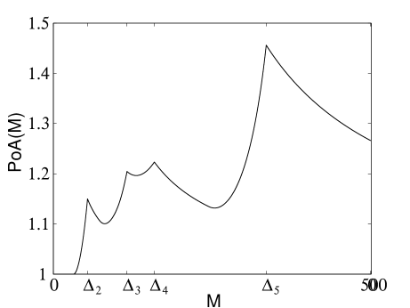
Figure 1: PoA vs $M$: the price of anarchy is maximized at one of the masses $\{\Delta_{2},\Delta_{3},\Delta_{4},\Delta_{5}\}$.

In the following, we give expression for the price of anarchy when the total population has mass $\Delta_{j},j\geq 2$. Let $m_{k},k<j$, be the mass of the population associated with BS $k$ under NE. From the definition of NE (see Definition II.4),

$$\frac{\gamma\sigma^{2}}{h_{k}(1-\gamma m_{k})}=\frac{\gamma\sigma^{2}}{h_{j}}\mbox{ for all }k<j.$$

Thus,

$$\Delta_{j}=\sum_{k<j}m_{k}=\frac{j-1}{\gamma}-\frac{h_{j}e_{j-1}}{\gamma}$$

where $e_{j}:=\sum_{k\leq j}\frac{1}{h_{k}}$ for $j\geq 1$. The cost at NE

$$C(\mathbf{m})=\sum_{k<j}m_{k}\frac{\gamma\sigma^{2}}{h_{j}}=\sigma^{2}\left(\frac{j-1}{h_{j}}-e_{j-1}\right).$$

Next, consider the system optimal congestion profile $\mathbf{m^{\ast}}$. It can be easily checked that $m^{\ast}_{k}$ is positive only if $k<j^{\prime}$ for a $j<j^{\prime}\leq N$. Moreover, it must be the case that

$$\sqrt{h_{k}}(1-\gamma m^{\ast}_{k}) = K\mbox{ for all }k<j^{\prime},$$

$$\mbox{and }\sqrt{h_{j^{\prime}}} \leq K,$$

for some constant $K>0$. Recall that $\sum_{k<j^{\prime}}m^{\ast}_{k}=\Delta_{j}$. Straightforward calculations yield that

$$K=\frac{j^{\prime}-j+h_{j}e_{j-1}}{e^{\ast}_{l-1}}$$

where $e^{\ast}_{j}:=\sum_{k\leq j}\frac{1}{\sqrt{h_{k}}}$ for $j\geq 1$. Moreover, $j^{\prime}$ is the least index satisfying

$$\sqrt{h_{j^{\prime}}}\leq\frac{j^{\prime}-j+h_{j}e_{j-1}}{e^{\ast}_{l-1}}.$$

The optimal cost, after substituting the values of $m^{\ast}_{k}$, turns out to be

$$C(\mathbf{m^{\ast}}) = \sum_{k<j^{\prime}}m^{\ast}_{k}\frac{\gamma\sigma^{2}}{h_{k}(1-m^{\ast}_{k}\gamma)}$$

$$= \sigma^{2}\left(\frac{e^{{\ast}^{2}}_{j^{\prime}-1}}{j^{\prime}-j+h_{j}e_{j-1}}-e_{j^{\prime}-1}\right).$$

The price of anarchy ${\rm PoA}(\Delta_{j})$ is the ratio $\frac{C(\mathbf{m})}{C(\mathbf{m^{\ast}})}$.

Finally, we show that the price of anarchy decreases with mass for $M\geq\Delta_{N}$. It can be easily checked that, for $M\geq\Delta_{N}$,

$${\rm PoA}(M) = \frac{e_{N}M\gamma}{e_{N}M\gamma-(e_{N}N-e^{{\ast}^{2}}_{N})}$$

$$= 1+\frac{e_{N}N-e^{{\ast}^{2}}_{N}}{e_{N}M\gamma-(e_{N}N-e^{{\ast}^{2}}_{N})}$$

from which the claim follows. Thus, to obtain a bound on the price of anarchy, we only focus on $M\leq\Delta_{N}$. For $M\leq\Delta_{N}$, the load on BS $j$

$$m_{j}\leq\frac{1}{\gamma}\left(1-\frac{h_{N}}{h_{j}}\right)$$

under NE. We use this observation in the next section.

B-C A Bound on the Price of Anarchy

Now, we derive a sharp bound on the price of anarchy for single class networks with arbitrary number of BSs, and gains $h_{j}\in[h_{\min},h_{\max}]$ for all the BSs. We follow Roughgarden [31, Chapter $3$].

In the BS association game, a generic cost function is of the form

$$c_{h}(m):=\frac{\sigma^{2}}{h}\frac{\gamma}{1-\gamma M},$$

and

$$\mathcal{C}:=\{c_{h}(\cdot):h\in[h_{\min},h_{\max}]\}$$

is the class of all feasible cost functions. Observe that the functions $c_{h}(\cdot)$ and the class $\mathcal{C}$ both are standard. We define

$$\bar{c}_{h}(m):=\frac{{\rm d}(mc_{h}(m)}{{\rm d}m}.$$

We also assume that the load on a BS with gain $h_{j}$ does not exceed

$$\theta_{h}:=\frac{1}{\gamma}\left(1-\frac{h_{\min}}{h}\right)$$

under NE. Thus, we redefine anarchy value for a cost function $c_{h}(\cdot)$ as

$$\alpha(c_{h}):=\sup_{m\leq\theta_{h}}[\lambda\mu+(1-\lambda)]^{-1}$$

where $\lambda\in(0,1)$ satisfies $\bar{c}_{h}(\lambda m)=c_{h}(m)$ and $\mu:=\frac{c_{h}(\lambda m)}{c_{h}(m)}\leq 1$. Both $\lambda$ and $\mu$ are functions of $m$; we do not show this dependence explicitly. Straightforward calculations yield that

$$\lambda = \frac{1-\sqrt{1-m\gamma}}{m\gamma},$$

$$\mu = \sqrt{1-m\gamma},$$

$$\mbox{and }\alpha(c_{h}) = \sup_{m\leq\theta_{h}}\frac{1}{2}\left[1-\frac{1}{1+\sqrt{1-m\gamma}}\right]^{-1}$$

$$= \frac{1}{2}\left(1+\sqrt{\frac{h}{h_{\min}}}\right).$$

The anarchy value for class $\mathcal{C}$ is (see [31, Definition 3.3.3])

$$\alpha(\mathcal{C})=\sup_{c_{h}\in\mathcal{C}}\alpha(c_{h})=\frac{1}{2}\left(1+\sqrt{\frac{h_{\max}}{h_{\min}}}\right)$$

It can be easily checked that [31, Theorem 3.3.8] remains valid with our new definition of anarchy value. Thus, price of anarchy is bounded by $\alpha(\mathcal{C})$. For any $0<\epsilon\leq\alpha(\mathcal{C})-1$, a price of anarchy $\geq\alpha(\mathcal{C})-\epsilon$ is realized in a network in which $(i)$ there is one BS with gain $h_{\max}$, $(ii)$ there are several BSs with gain $h_{\min}$ (minimum number depending on $\epsilon$), and $(iii)$ the population has mass $\theta_{h_{\max}}$ (see the proof of [31, Lemma 3.4.3] for details).

References

• [1] G. J. Foschini and Z. Miljanic, “A simple distributed autonomous power control algorithm and its convergence,” IEEE Trans. On Vehicular Technology, vol. 42, no. 4, pp. 641–646, November 1993.
• [2] R. D. Yates, “A framework for uplink power control in cellular radio systems,” IEEE J. Select. Areas Commun., vol. 13, no. 7, pp. 1341–1347, September 1995.
• [3] S. V. Hanly, “An algorithm for combined cell-site selection and power control to maximize cellular spread spectrum capacity,” IEEE J. Select. Areas Commun., vol. 13, no. 7, pp. 1332–1340, September 1995, invited Paper.
• [4] M. Chiang, P. Hande, T. Lan, and C. W. Tan, Power Control in Wireless Cellular Networks.   NOW Publishers, 2008.
• [5] G. Scutari, S. Barbarossa, and D. P. Palomar, “Potential games: A framework for vector power control problems with coupled constraints,” in IEEE International Conference on Acoustics, Speech and Signal Processing (ICASSP), vol. 4, May 2006, pp. IV–241–IV–244.
• [6] T. Heikkinen, “A potential game approach to distributed power control and scheduling,” Computer Networks, vol. 50, no. 13, pp. 2295–2311, September 2006.
• [7] E. Altman and Z. Altman, “S-modular games and power control in wireless networks,” IEEE Transactions on Automatic Control, vol. 48, no. 5, pp. 839–842, May 2003.
• [8] L. Jiang, S. Parekh, and J. Walrand, “Base station association game in multi-cell wireless networks,” in IEEE Wireless Communication and Networking Conference, March–April 2008, pp. 1616–1621.
• [9] D. Monderer and L. S. Shapley, “Potential games,” Games and Economic Behavior, vol. 14, no. 1, pp. 124–143, May 1996.
• [10] J. O. Neel, “Analysis and design of cognitive radio networks and distributed radio resource management algorithms,” Ph.D. dissertation, Virginia Polytechnic Institute and State University, Blacksburg, VA, September 2006.
• [11] I. Milchtaich, “Congestion games with player-specific payoff functions,” Games and Economic Behavior, vol. 13, no. 1, pp. 111–124, March 1996.
• [12] M. Voorneveld, “Best-response potential games,” Economics Letters, vol. 66, pp. 289–295, 2000.
• [13] R. W. Rosenthal, “A class of games possessing pure-strategy nash equilibria,” International Journal of Game Theory, vol. 2, no. 1, pp. 65–67, December 1973.
• [14] M. Gairing, B. Monien, and K. Tiemann, Routing (Un-) Splittable Flow in Games with Player-Specific Linear Latency Functions, ser. LNCS.   Springer Berlin / Heidelberg, 2006, vol. 4051, pp. 501–512.
• [15] C. Georgiou, T. Pavlides, and A. Philippou, “Selfish routing in the presence of network uncertainty,” Parallel Processing Letters, vol. 19, no. 1, pp. 141–157, March 2009.
• [16] M. Mavronicolas, I. Milchtaich, B. Monien, and K. Tiemann, “Congestion games with player-specific constants,” in Mathematical Foundations of Computer Science, ser. Lecture Notes in Computer Science.   Springer Berlin/Heidelberg, August 2007, pp. 633–644.
• [17] W. H. Sandholm, “Potential games with continuous player sets,” Journal of Economic Theory, 2001.
• [18] M. Beckman, C. B. McGuire, and C. B. Winsten, Studies in the Economics of Transportation.   New Haven: Yale University Press, 1956.
• [19] S. C. Dafermos and F. T. Sparrow, “The traffic assignment problem for a general network,” Journal of Research of the National Bureau of Standards, Series B, vol. 73B, no. 2, pp. 91–118, 1969.
• [20] S. C. Dafermos, “The traffic assignment problem for multi-class user transportation networks,” Transportation Science, vol. 6, no. 1, pp. 73–87, February 1972.
• [21] M. J. Smith, “The marginal cost taxation of a transportation network,” Transportation Research, vol. 13B, pp. 237–242, 1979.
• [22] T. Roughgarden and E. Tardos, “How bad is selfish routing?” Journal of the ACM, vol. 49, no. 2, pp. 236–259, March 2002.
• [23] I. Caragiannis, C. Kaklamanis, and P. Kanellopoulos, “Taxes for linear atomic congestion games,” in Proceedings of the 14th conference on Annual European Symposium, vol. 14, Zurich, Switzerland, September 2006, pp. 184–195.
• [24] D. Fotakis and P. G. Spirakis, “Cost-balancing tolls for atomic network congestion games,” in Proceedings of the 3rd international conference on Internet and network economics (WINE), San Diego, CA, USA, December 2007, pp. 179–190.
• [25] A. Kumar, D. Manjunath, and J. Kuri, Wireless Networking.   Morgan Kaufman Publishers, 2008.
• [26] J. Aspnes, C. Busch, S. Dolev, P. Fatourou, C. Georgiou, A. Shvartsman, P. Spirakis, and R. Wattenhofer, “Eight open problems in distributed computing,” Bulletin of the European Association for Theoretical Computer Science, vol. 90, pp. 109–126, October 2006.
• [27] A. W. Marshall and I. Olkin, Inequalities : Theory of Majorization and Its Applications.   Academic Press, New York, December 1979.
• [28] S. Boyd and L. Vandenberghe, Convex Optimization.   Cambridge, UK: Cambridge University Press, 2004.
• [29] I. Milchtaich, “Generic uniqueness of equilibrium in large crowding games,” Mathematics of Operations Research, vol. 25, no. 3, pp. 349–364, August 2000.
• [30] D. Fotakis and P. G. Spirakis, “Cost-balancing tolls for atomic network congestion games,” in Third International Workshop on Internet and Network Economics, San Diego, CA, USA.   Springer, December 2007, pp. 179–190.
• [31] T. Roughgarden, “Selfish routing,” Ph.D. dissertation, Cornell University, May 2002.
• [32] C. Singh, “Marginal cost pricing for atomic network congestion games,” Indian Institute of Science, Bangalore, India, Tech. Rep., November 2011, http://ece.iisc.ernet.in/$\sim$chandra/publications.html.
• [33] E. Koutsoupias and C. Papadimitriou, “Worst-case equilibria,” in Proceedings of the 16th Annual Symposium on Theoretical Aspects of Computer Science (STACS), Trier, Germany, March 1999, pp. 404–413.
• [34] C. Papadimitriou, “Algorithms, games, and the internet,” in Proceedings of the thirty-third annual ACM symposium on Theory of computing, Hersonissos, Greece, 2001, pp. 749–753.