Bilocal phase operators in $\beta$-deformed super Yang-Mills

Abstract

We present tree-level scattering amplitudes in $\beta$-deformed super Yang-Mills theory in terms of new generating functions, derived by construction of a phase operator and application thereof to the $\mathcal{N}=4$ superamplitudes. The technique is explicitly illustrated for the MHV and NMHV sectors. Along these lines we propose a phase representation of the $\mathcal{N}=4$ superconformal algebra realized on deformed amplitudes in the planar limit. Validity of the MHV vertex expansion is proven and a connection to non-planar multi-loop unitarity cuts is established. Our derivations are also compatible with the related $\gamma$-deformation.

I Introduction

Maximally supersymmetric ($\mathcal{N}=4$) super Yang-Mills theory in four dimensions is a very special quantum field theory in several ways. First of all, it has surprisingly simple and well-behaved amplitudes. The $\mathcal{N}=4$ supermultiplet is CPT self-conjugate and in addition the theory is both classically and quantum mechanically conformally invariant because the renormalization group $\beta$-function vanishes identically. Even more remarkably, although gravitational interactions are absent, the $\mathcal{N}=4$ theory is intimately related to a supergravity theory via the celebrated AdS/CFT correspondence.

Multiloop $\mathcal{N}=4$ scattering amplitudes are very elegantly studied within the on-shell superspace formalism Bern:2009xq ; Sogaard:2011pr ; Bianchi:2008pu ; Elvang:2008na ; Georgiou:2004by ; Elvang:2008vz ; Elvang:2011fx ; ArkaniHamed:2008gz ; Drummond:2008vq ; Brandhuber:2008pf ; Drummond:2008cr ; Drummond:2009fd ; Drummond:2008bq . The principle is to arrange the entire supermultiplet as a superfield expanded in Grassmann variables. All possible scattering combinations are realized by formation of superamplitudes, defined as generating functions of $n$ copies of superfields corresponding to the external legs. Single amplitudes are then projected out by unique strings of Grassmann differential operators or pieced together in a graphical framework. Superamplitudes for general particle and helicity configurations may be constructed with the Britto-Cachazo-Feng-Witten (BCFW) on-shell recursion relations Britto:2004ap ; Britto:2005fq ; ArkaniHamed:2008gz ; Brandhuber:2008pf .

It is of course very interesting to examine features of the $\mathcal{N}=4$ theory in more general settings. Super Yang-Mills theories with less than maximal supersymmetry do not possess all of the amazing properties mentioned, although the superspace formalism can be generalized Elvang:2011fx ; Lal:2009gn ; Sogaard:2011pr . However, exactly marginal deformations of the $\mathcal{N}=4$ super Yang-Mills theory preserving only reduced amount of supersymmetry in particular inherit conformal invariance Leigh:1995ep , and have recently attracted considerable attention especially catalyzed by the AdS/CFT duality. Exactly marginal deformations have also been subject to intense investigations within the perturbative regime Khoze:2005nd ; Mansson:2008xv ; Lunin:2005jy ; Ananth:2006ac ; Ananth:2007px ; Elmetti:2006gr ; Elmetti:2007up ; Kazakov:2007dy ; Ihry:2008gm ; Bork:2007bj ; Oz:2007qr ; Mauri:2005pa ; Fiamberti:2010fw ; Madhu:2007ew ; Kulaxizi:2006zc ; Bundzik:2006jz . In particular, it has been of special interest to understand how scattering amplitudes are modified by the so-called $\beta$-deformation. It can be shown that conformal invariance of the planar $\beta$-deformed super Yang-Mills theory requires reality of $\beta$, the deformation parameter. The theory enjoys only $\mathcal{N}=1$ supersymmetry and a global $U(1)_{1}\times U(1)_{2}$ flavor symmetry, and may be formulated with both symmetries manifest in the $\mathcal{N}=1$ superspace formalism in terms of three charged chiral superfields and neutral vector superfield, and a star product operation which incorporates the charges of the fields under the flavor symmetry. Using this Lagrangian approach the $\beta$-deformed Feynman rules of the deformed theory may be obtained, and the behaviour of its scattering amplitudes elucidated Khoze:2005nd . It turns out that the $\mathcal{N}=4$ and $\beta$-deformed theories are very similar.

Motivated by the developments in exactly marginal deformations and inspired by how powerfully on-shell scattering amplitudes are constructed from analyticity and unitarity in the $\mathcal{N}=4$ on-shell framework, we recast the deformed theory in terms of generating functions.

II Notation and conventions

Several modern techniques apply to present gauge theory scattering amplitudes very effectively. With all states in the adjoint representation of the gauge group, say $SU(N_{c})$, any tree-level amplitude can be color decomposed as

$${\mathbb{A}}^{\textrm{tree}}_{n}(1,2,\dots,n)=g^{n-2}\sum_{\sigma\in S_{n}/Z_{n}}\operatorname{Tr}\left(T^{a_{\sigma(1)}}T^{a_{\sigma(2)}}\cdots T^{a_{\sigma(n)}}\right)A_{n}^{\textrm{tree}}(\sigma(1),\sigma(2),\dots,\sigma(n))\;,$$ (1)

where $g$ is the gauge coupling constant and $A_{n}^{\textrm{tree}}(\sigma(1),\sigma(2),\dots,\sigma(n))$ are partial amplitudes soaking up the entire kinematical structure corresponding to a particular ordering of the $n$ external legs encoded by the trace of the gauge group generators $T^{a}$. The sum is over all permutations $S_{n}$ with trace preserving cyclic permutations $Z_{n}$ modded out.

The partial amplitudes are written in terms of Lorentz invariant, little group covariant holomorphic and antiholomorphic spinor products. In order to distinguish the two chiralities we use angle and square brackets, and define

$$\langle ij\rangle=-\langle ji\rangle\equiv\epsilon_{\alpha\beta}\lambda_{i}^{\alpha}\lambda_{j}^{\beta}\;,\quad[ij]=-[ji]\equiv\epsilon_{\dot{\alpha}\dot{\beta}}\tilde{\lambda}_{i}^{\dot{\alpha}}\tilde{\lambda}_{j}^{\dot{\beta}}$$ (2)

for commuting spinors $\lambda_{i}^{\alpha}$ and $\tilde{\lambda}_{i}^{\dot{\alpha}}$ related to momentum by $p_{i}^{\alpha\dot{\alpha}}=\lambda_{i}^{\alpha}\lambda_{i}^{\dot{\alpha}}$.

III On-shell $\mathcal{N}=4$ supersymmetry

The $\mathcal{N}=4$ gauge multiplet has the unique property of CPT self-conjugacy which implies that all on-shell states can be assembled by a single holomorphic superfield $\Phi(p,\eta)$. It is expanded in Grassmann variables $\eta_{a}$ where $a=1,\dots,4$ is a fundamental index of $SU(4)_{R}$, the $R$-symmetry group of the theory. Within this setup the sixteen physical states transform in $r$-rank antisymmetric tensor representations as two gluons $g_{+}$ and $g^{abcd}_{-}$, four fermion pairs $f^{a}_{+}$ and $f^{abc}_{-}$, plus six real scalars $s^{ab}$. The tensor rank $r$ and particle helicity $h$ are related through $2h=2-r$.

The superfield is Drummond:2008cr (repeated indices are summed)

$$\Phi(p,\eta)=g_{+}+\eta_{a}f^{a}_{+}+\frac{1}{2!}\eta_{a}\eta_{b}s^{ab}+\frac{1}{3!}\eta_{a}\eta_{b}\eta_{c}f^{abc}_{-}+\frac{1}{4!}\eta_{a}\eta_{b}\eta_{c}\eta_{d}g^{abcd}_{-}\;.$$ (3)

There also exists an antiholomorphic superfield

$$\tilde{\Phi}(p,\tilde{\eta})=g^{-}+\tilde{\eta}^{a}f_{a}^{-}+\frac{1}{2!}\tilde{\eta}^{a}\tilde{\eta}^{b}s_{ab}+\frac{1}{3!}\tilde{\eta}^{a}\tilde{\eta}^{b}\tilde{\eta}^{c}f^{+}_{abc}+\frac{1}{4!}\tilde{\eta}^{a}\tilde{\eta}^{b}\tilde{\eta}^{c}\tilde{\eta}^{d}g^{+}_{abcd}\;,$$ (4)

linked to $\Phi(p,\eta)$ by the Grassmann Fourier transform, but with the exact same particle content encoded. Due to this equivalence either representation may be preferred. In this paper we reserve the holomorphic and antiholomorphic descriptions for $\mathrm{MHV}$ and $\overline{\mathrm{MHV}}$ amplitudes respectively.

III.1 MHV superamplitudes

Proliferation of scattering amplitudes in $\mathcal{N}=4$ super Yang-Mills theory is handled by introduction of superamplitudes, which are functions of $n$ copies of the superfield, one for each external leg. The full $n$-point tree-level superamplitude is organized ascendingly according to Grassmann degree in steps of four,

$$\mathcal{A}_{n}(\lambda,\tilde{\lambda},\eta)=\mathcal{A}(\Phi_{1}\cdots\Phi_{n})=\mathcal{A}_{n}^{\mathrm{MHV}}+\mathcal{A}_{n}^{\mathrm{NMHV}}+\cdots+\mathcal{A}_{n}^{\overline{\mathrm{MHV}}}\;,$$ (5)

ranging from eight $\eta$’s to $4n-8$. It follows in particular that all MHV amplitudes may be packaged into a generating function, also referred to as the MHV superamplitude. Each term thus corresponds to a regular scattering amplitude involving gluons, fermions and scalars. It is convention to extract the MHV sector from the full superamplitude as an overall factor.

The MHV tree-level superamplitude is in addition to the well-known overall momentum conservation proportional to an eightfold Grassmann delta function conserving total supermomentum $Q^{\alpha}_{a}\equiv\sum_{j=1}^{n}\lambda_{j}^{\alpha}\eta_{ja}$, and is defined by Bern:2009xq

$$\mathcal{A}^{\mathrm{MHV}}_{n}=i\frac{(2\pi)^{4}\delta^{(4)}(\sum_{i=1}^{n}p_{i})}{\prod_{r=1}^{n}\langle r(r+1)\rangle}\delta^{(8)}\bigg{(}\sum_{j=1}^{n}\lambda_{j}^{\alpha}\eta_{ja}\bigg{)}\;.$$ (6)

For calculational purposes it proves advantageous to expand the Grassmann delta function present in the MHV superamplitude as a sum of monomials in the $\eta$’s, first in all possible values of the group index,

$$\delta^{(8)}\bigg{(}\sum_{j=1}^{n}\lambda_{j}^{\alpha}\eta_{ja}\bigg{)}=\prod_{a=1}^{4}\delta^{(2)}\bigg{(}\sum_{j=1}^{n}\lambda_{j}^{\alpha}\eta_{ja}\bigg{)}\;,$$ (7)

and then using $\delta(\eta)=\eta$ for Grassmann variables,

$$\delta^{(8)}\bigg{(}\sum_{j=1}^{n}\lambda_{j}^{\alpha}\eta_{ja}\bigg{)}=\prod_{a=1}^{4}\sum_{i<j}\langle ij\rangle\eta_{ia}\eta_{ja}\;.$$ (8)

Frequently we write holomorphic and antiholomorphic spinor products of supermomenta of the individual legs defined by

$$\langle q_{ia}q_{ja}\rangle\equiv\eta_{ia}\langle ij\rangle\eta_{ja}\;,\qquad[\tilde{q}_{i}^{a}\tilde{q}_{j}^{a}]\equiv\tilde{\eta}_{i}^{a}[ij]\tilde{\eta}_{j}^{a}\;.$$ (9)

Consequently, the MHV generating function reaches the very clean form

$$\mathcal{A}^{\mathrm{MHV}}_{n}=i\frac{\prod_{a=1}^{4}\sum_{i<j}\langle q_{ia}q_{ja}\rangle}{\prod_{r=1}^{n}\langle r(r+1)\rangle}\;,$$ (10)

with four-momentum conservation stripped.

For four external legs, some simple examples of MHV component amplitudes are

$$A_{4}^{\mathrm{MHV}}(1^{-}_{g^{1234}},2^{-}_{g^{1234}},3^{+}_{g},4^{+}_{g}) =i\frac{\prod_{a=1}^{4}\langle q_{1a}q_{2a}\rangle}{\langle 12\rangle\langle 23\rangle\langle 34\rangle\langle 41\rangle}\;,$$ (11)

$$A_{4}^{\mathrm{MHV}}(1^{-}_{g^{abcd}},2^{-}_{f^{abc}},3^{+}_{f^{d}},4^{+}_{g}) =i\frac{\langle q_{1a}q_{2a}\rangle\langle q_{1b}q_{2b}\rangle\langle q_{1c}q_{2c}\rangle\langle q_{1d}q_{3d}\rangle}{\langle 12\rangle\langle 23\rangle\langle 34\rangle\langle 41\rangle}\;,$$ (12)

$$A_{4}^{\mathrm{MHV}}(1^{-}_{f^{abc}},2^{-}_{f^{abd}},3_{s^{cd}},4^{+}_{g}) =i\frac{\langle q_{1a}q_{2a}\rangle\langle q_{1b}q_{2b}\rangle\langle q_{1c}q_{3c}\rangle\langle q_{2d}q_{3d}\rangle}{\langle 12\rangle\langle 23\rangle\langle 34\rangle\langle 41\rangle}\;.$$ (13)

Analogous to the MHV superamplitude we may use the antiholomorphic superfields (4) to build a $\overline{\mathrm{MHV}}$ generating function. The $\overline{\mathrm{MHV}}$ superamplitude conserves total conjugate supermomentum $\tilde{Q}^{\dot{\alpha}a}=\sum_{i=1}^{n}\tilde{\lambda}_{i}^{\dot{\alpha}}\tilde{\eta}_{i}^{a}$ and is apart from an ordinary momentum conserving delta function given by

$$\mathcal{A}^{\mathrm{\overline{\mathrm{MHV}}}}_{n}=i(-1)^{n}\frac{\delta^{(8)}(\sum_{i=1}^{n}\tilde{\lambda}_{i}^{\dot{\alpha}}\tilde{\eta}_{i}^{a})}{\prod_{r=1}^{n}[r(r+1)]}=i(-1)^{n}\frac{\prod_{a=1}^{4}\sum_{i<j}[\tilde{q}_{i}^{a}\tilde{q}_{j}^{a}]}{\prod_{r=1}^{n}[r(r+1)]}\;.$$ (14)

It is mapped from the $\tilde{\eta}$-coordinates to the untilded superspace using the Grassmann Fourier transform realized by the $n$-leg operator

$$\hat{\mathcal{F}}\bullet\equiv\int\prod_{i,a}d\tilde{\eta}_{i}^{a}\exp\left(\sum_{b,j}\tilde{\eta}^{b}_{j}\eta_{jb}\right)\bullet\;.$$ (15)

As a first example of $\overline{\mathrm{MHV}}$ component amplitudes consider the equivalent reinterpretation of the MHV amplitudes (11)-(13) in the tilded superspace,

$$A_{4}^{\overline{\mathrm{MHV}}}(1^{-}_{g},2^{-}_{g},3^{+}_{g_{1234}},4^{+}_{g_{1234}}) =i\frac{\prod_{a=1}^{4}[\tilde{q}_{3}^{a}\tilde{q}_{4}^{a}]}{[12][23][34][41]}\;,$$ (16)

$$A_{4}^{\overline{\mathrm{MHV}}}(1^{-}_{g},2^{-}_{f_{d}},3^{+}_{f_{abc}},4^{+}_{g_{abcd}}) =i\frac{[\tilde{q}_{3a}\tilde{q}_{4a}][\tilde{q}_{3b}\tilde{q}_{4b}][\tilde{q}_{3c}\tilde{q}_{4c}][\tilde{q}_{2d}\tilde{q}_{4d}]}{[12][23][34][41]}\;,$$ (17)

$$A_{4}^{\overline{\mathrm{MHV}}}(1^{-}_{f_{d}},2^{-}_{f_{c}},3_{s_{ab}},4^{+}_{g_{abcd}}) =i\frac{[\tilde{q}_{3a}\tilde{q}_{4a}][\tilde{q}_{3b}\tilde{q}_{4b}][\tilde{q}_{2c}\tilde{q}_{4c}][\tilde{q}_{1d}\tilde{q}_{4d}]}{[12][23][34][41]}\;.$$ (18)

III.2 The NMHV sector

The supersymmetric BCFW recursion relations ArkaniHamed:2008gz ; Brandhuber:2008pf generate all tree-level superamplitudes in $\mathcal{N}=4$ super Yang-Mills theory in terms of nested sums of dual superconformal invariants Drummond:2008cr from just $\mathrm{MHV}$ and $\overline{\mathrm{MHV}}$ amplitudes. The essense is to deform the on-shell superspace by a supershift and recover the physical amplitude by residue calculus. In this paper it suffices to examine in detail only the $\mathrm{NMHV}$ superamplitude. It comes with the very compact result Drummond:2008cr

$$\mathcal{A}_{n}^{\mathrm{NMHV}}=\mathcal{A}_{n}^{\mathrm{MHV}}\sum_{1<s<t<n}R_{n;st}\;,$$ (19)

where, however, $R_{n;st}$ are complicated dual superconformal invariants (see e.g. Drummond:2008vq ),

$$R_{n;st}=\frac{\langle s(s-1)\rangle\langle t(t-1)\rangle\delta^{(4)}(\Xi_{n;st})}{x_{st}^{2}\langle n|x_{ns}x_{st}|t\rangle\langle n|x_{ns}x_{st}|t-1\rangle\langle n|x_{nt}x_{ts}|s\rangle\langle n|x_{nt}x_{ts}|s-1\rangle}\;,$$ (20)

depending on another intricate Grassmann valued object, $\Xi_{n;st}$, defined by

$$\Xi_{n;st}=\sum_{i=t}^{n-1}\langle n|x_{ns}x_{st}|i\rangle\eta_{ia}+\sum_{i=s}^{n-1}\langle n|x_{nt}x_{ts}|i\rangle\eta_{ia}\;.$$ (21)

Equipped with all necessary machinery of $\mathcal{N}=4$ superamplitudes we are now ready to consider applications in $\beta$-deformed super Yang-Mills theory.

IV $\beta$-deformed super Yang-Mills theory

Marginal deformations of conformally invariant supersymmetric gauge theories were first systematically studied by Leigh and Strassler Leigh:1995ep , and have subsequently been analyzed extensively both perturbatively and at strong coupling in Khoze:2005nd ; Mansson:2008xv ; Lunin:2005jy ; Mauri:2005pa ; Ananth:2006ac ; Ananth:2007px ; Elmetti:2006gr ; Elmetti:2007up ; Kazakov:2007dy ; Ihry:2008gm ; Bork:2007bj ; Oz:2007qr ; Fiamberti:2010fw ; Madhu:2007ew ; Kulaxizi:2006zc ; Bundzik:2006jz just to mention a few.

Before exactly marginal deformations are treated, we shall first pay brief attention to the Lagrangian formulation of the undeformed $\mathcal{N}=4$ super Yang-Mills theory. The standard $\mathcal{N}=1$ superspace formalism applies by construction to field theories with $\mathcal{N}=1$ supersymmetry. But since $\mathcal{N}>1$ supersymmetric theories may be reduced to multiple unextended supermultiplets coupled together, the $\mathcal{N}=1$ framework proves useful in a much richer class of theories. The $\mathcal{N}=4$ particle content decomposes into one $\mathcal{N}=1$ vector multiplet and three $\mathcal{N}=1$ chiral multiplets. The Lagrangian can be written Gates:1983nr ; Fiamberti:2010fw

$$\mathcal{L}_{\mathcal{N}=4}= \int d^{2}\theta d^{2}\bar{\theta}\operatorname{Tr}e^{-gV}\bar{\Phi}^{i}e^{gV}\Phi_{i}$$

$${}+\frac{1}{2g^{2}}\int d^{2}\theta\operatorname{Tr}W^{\alpha}W_{\alpha}+\left\{g\int d^{2}\theta\operatorname{Tr}\Phi_{1}[\Phi_{2},\Phi_{3}]+\mathrm{h.c.}\right\}\;,$$ (22)

where $V$ is the vector superfield and $\Phi_{1}$, $\Phi_{2}$ and $\Phi_{3}$ are the three chiral superfields. The kinetic term for the vector superfield involves as usual the superfield strength defined by $W_{\alpha}=i\bar{\mathcal{D}}^{2}(e^{-gV}\mathcal{D}_{\alpha}e^{gV})$ where $\mathcal{D}_{\alpha}$ and $\bar{\mathcal{D}}_{\dot{\alpha}}$ are supercovariant derivatives. This Lagrangian is manifestly $\mathcal{N}=1$ supersymmetric being constructed using the $\mathcal{N}=1$ superspace prescription. Moreover, the three chiral superfields enjoy manifest $SU(3)$ flavor symmetry, but the full $SU(4)$ $R$-symmetry is obscured.

The general Leigh-Strassler theory is parametrized by complexification of the gauge coupling $g$ and modification of the superpotential by the substitution

$$g\operatorname{Tr}\left(\Phi_{1}\Phi_{2}\Phi_{3}-\Phi_{1}\Phi_{3}\Phi_{2}\right)\mapsto\kappa\operatorname{Tr}\left(q\Phi_{1}\Phi_{2}\Phi_{3}-q^{-1}\Phi_{1}\Phi_{3}\Phi_{2}\right)+\rho\operatorname{Tr}\left(\Phi_{1}^{3}+\Phi_{2}^{3}+\Phi_{3}^{3}\right)\;,$$ (23)

for complex $\kappa,\rho$ and $q$. The deformations break supersymmetry to $\mathcal{N}=1$. In order for the deformation to become exactly marginal and thereby inherit finiteness at the quantum level, the parameters must be highly constrained. Leigh and Strassler demonstrated the existence of a three-complex dimensional surface in the coupling constant space of conformally invariant theories with $\mathcal{N}=1$ supersymmetry. This surface can be defined as a quite complicated level set $\gamma(\kappa,\rho,q,g)=0$. The condition however has to be calculated perturbatively and unfortunately its form is not known beyond few loops except for very restrictive choices of the couplings.

IV.1 Star product induced $\beta$-deformations

The Leigh-Strassler deformed theory generated by the superpotential substitution (23) includes as a special case a one-parameter family of theories known as $\beta$-deformations, which extend to quantum finiteness to all orders in the planar limit Mauri:2005pa . The model follows by tightening the assumptions on the parameters and setting $\kappa=g$, $\rho=0$ and $q\bar{q}=1$, so that for $\beta_{R}$ real, the new superpotential becomes

$$\mathcal{W}_{\beta}=g\operatorname{Tr}\left(e^{i\pi\beta_{R}}\Phi_{1}\Phi_{2}\Phi_{3}-e^{-i\pi\beta_{R}}\Phi_{1}\Phi_{3}\Phi_{2}\right)\;,$$ (24)

whence the undeformed theory is recovered by sending $e^{i\pi\beta_{R}}\to 1$.

It turns out that the $\beta$-deformation can be understood in terms of a special operation between the superfields, namely the star product, which will prove invaluable when we evaluate deformations of scattering amplitudes Khoze:2005nd . In order to define the star product it is necessary to discuss the left-over symmetries of the $\beta$-deformed Lagrangian. The original $R$-symmetry is broken from $SU(4)_{R}$ to $U(1)_{R}$, but it is observed that the deformed theory in addition is invariant under a global $U(1)_{1}\times U(1)_{2}$ flavor symmetry of the three chiral superfields. More specifically the symmetries can be expressed as

$$U(1)_{1}:\;\;(\Phi_{1},\Phi_{2},\Phi_{3},V)\mapsto(\Phi_{1},e^{i\alpha_{1}}\Phi_{2},e^{-i\alpha_{1}}\Phi_{3},V)\;,$$

$$U(1)_{2}:\;\;(\Phi_{1},\Phi_{2},\Phi_{3},V)\mapsto(e^{-i\alpha_{2}}\Phi_{1},e^{i\alpha_{2}}\Phi_{2},\Phi_{3},V)\;,$$ (25)

the vector superfield being neutral under these transformations. The symmetry charges are

$$Q^{[1]}\equiv(0,+1,-1,0)\;,\quad\;\;Q^{[2]}\equiv(-1,+1,0,0)\;.$$ (26)

Suppose that $\Phi_{i}$ and $\Phi_{j}$ are chiral superfields with flavor symmetry charges $Q^{[1,2]}_{i}$ and $Q^{[1,2]}_{j}$ respectively. Then the star product operation together with the $\beta$-deformed commutator between these fields is defined by

$$\Phi_{i}\star\Phi_{j}\equiv e^{i\pi\beta_{R}\left(Q_{i}^{[1]}Q_{j}^{[2]}-Q_{i}^{[2]}Q_{j}^{[1]}\right)}\Phi_{i}\Phi_{j}\;,\quad[\Phi_{i},\Phi_{j}]_{\beta}\equiv e^{i\pi\beta_{ij}}\Phi_{i}\Phi_{j}-e^{-i\pi\beta_{ij}}\Phi_{j}\Phi_{i}\;,$$ (27)

where $\beta_{ij}$ is the antisymmetric matrix

$$\beta_{ij}=-\beta_{ji}\;,\quad\beta_{12}=-\beta_{13}=\beta_{23}\equiv\beta_{R}\;.$$ (28)

For $\beta_{R}$ real it follows that the star product is simply the usual product adjusted by an overall flavor dependent phase factor. Of important properties of the star product we mention associativity, which is a consequence of additivity of the flavor charges, and noncommutativity, the latter being obvious from the definition (27).

Prior to implementation in the $\mathcal{N}=4$ Lagrangian the star product must extend to the antichiral superfields $\bar{\Phi}_{1}$, $\bar{\Phi}_{2}$ and $\bar{\Phi}_{3}$. They carry opposite charges to the chiral superfields under the $U(1)_{1}\times U(1)_{2}$ symmetry so that $\Phi_{i}\bar{\Phi}_{i}$ is chargeless and $\Phi_{i}\star\bar{\Phi}_{i}=\Phi_{i}\bar{\Phi}_{i}$. We therefore note

$$\bar{Q}^{[1]}\equiv(0,-1,+1,0)=-Q^{[1]}\;,\quad\;\;\bar{Q}^{[2]}\equiv(+1,-1,0,0)=-Q^{[2]}\;,$$ (29)

whereby both antichirality and mixed chirality star products become well defined.

With this operation the $\beta$-deformation can be induced in the $\mathcal{N}=4$ Lagrangian by substituting all ordinary products between superfields with star products, or equivalently replacing all commutators with $\beta$-deformed brackets. In particular, the superpotential can be written

$$\mathcal{W}_{\beta}=g\operatorname{Tr}\left(\Phi_{1}\star\Phi_{2}\star\Phi_{3}-\Phi_{1}\star\Phi_{3}\star\Phi_{2}\right)=g\operatorname{Tr}\left(e^{i\pi\beta_{R}}\Phi_{1}\Phi_{2}\Phi_{3}-e^{-i\pi\beta_{R}}\Phi_{1}\Phi_{3}\Phi_{2}\right)\;,$$ (30)

and hence the $\beta$-deformed Lagrangian takes the form

$$\mathcal{L}_{\beta}= \int d^{2}\theta d^{2}\bar{\theta}\operatorname{Tr}e^{-gV}\bar{\Phi}^{i}e^{gV}\Phi_{i}$$

$${}+\frac{1}{2g^{2}}\int d^{2}\theta\operatorname{Tr}W^{\alpha}W_{\alpha}+\left\{g\int d^{2}\theta\operatorname{Tr}\Phi_{1}[\Phi_{2},\Phi_{3}]_{\beta}+\mathrm{h.c.}\right\}\;.$$ (31)

By consideration of the component version of the Lagrangian for the $\mathcal{N}=4$ super Yang-Mills theory rather than its superspace representation (IV) it is elementary to derive the modified color-ordered Feynman rules. We mention that non-consecutive four-scalar interactions and Yukawa vertices without particles from the vector multiplet exhaust the $\beta$-deformed vertices (see fig. 1), and refer the reader to Khoze:2005nd for detailed calculations.

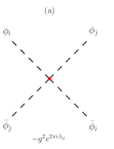
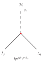
Figure 1: The $\beta$-deformation adds overall phase factors to the original vertex rules of the depicted four-scalar and Yukawa couplings. We denote the three complex scalar field components of the chiral superfields $\Phi_{i}$ by $\phi_{i}$, while $\lambda_{i}$ label their fermionic superpartners. Notice that the ordering of the legs is crucial.

IV.2 Phase structure and effective vertices

Scattering amplitudes in $\mathcal{N}=4$ and $\beta$-deformed super Yang-Mills theories seem closely related when comparing their Feynman rules. Indeed, only three specific four-scalar and Yukawa interactions are modified, and this deformation introduces nothing but prefactors to the vertex rules. Several comments are important in this connection.

The two theories have the same particle content and it is easy to see that many amplitudes are actually identical. For a $\beta$-deformed amplitude to agree with the corresponding $\mathcal{N}=4$ expression, the phases of the $\beta$-dependent vertices should cancel each other, or such vertices should simply be absent in the diagram. Whole classes of amplitudes are insensitive to the phase deformation, the most obvious being all tree-level amplitudes with external gluons and gluinos exclusively.

In general, amplitudes in the deformed theory are $\beta$-dependent. The modifications however turn out to be surprisingly uncomplicated. At first we realize that the original and deformed theories are equivalent at tree-level, up to a multiplicative prefactor. This conclusion follows from the simplicity of the color-ordered Feynman vertices. But it can be shown that the product of phase factors from the individual vertices is independent of the internal structure of the diagram. Suppose the arbitrary color-ordered tree-level amplitude in consideration has any combination of $n$ external fields and label them $\Lambda_{1},\Lambda_{2},\dots,\Lambda_{n}$. Then the $\beta$-dependence of this amplitude is entirely captured by $\operatorname{Tr}\left[\Lambda_{1}\star\Lambda_{2}\star\cdots\star\Lambda_{n}\right]$. Actually this statement applies not only to tree-level amplitudes, but is guaranteed to hold to all orders in perturbation theory in the planar limit. The claim has profound consequences for our applications of $\beta$-deformed super Yang-Mills theory. A proof based on effective vertices of only external legs was provided in Khoze:2005nd . Shortly we report a similar strategy for supervertices.

We end this section by deriving an expression for the phase factor of any given $n$-point amplitude in terms of only the $U(1)_{1}\times U(1)_{2}$ charges of the superfields corresponding to the external legs. Upon invoking the definition of the star product (27) we deduce the generalization to $n$ legs,

$$\mathcal{P}^{\beta_{R}}\left(\Lambda_{1},\Lambda_{2},\dots,\Lambda_{n}\right) \equiv\frac{\operatorname{Tr}\left[\Lambda_{1}\star\Lambda_{2}\star\cdots\star\Lambda_{n}\right]}{\operatorname{Tr}\left[\Lambda_{1}\Lambda_{2}\cdots\Lambda_{n}\right]}$$

$$=\prod_{i=1}^{n-1}\exp\bigg{[}i\pi\beta_{R}\sum_{j=i+1}^{n}\left(Q^{[1]}_{\Lambda_{i}}Q^{[2]}_{\Lambda_{j}}-Q^{[2]}_{\Lambda_{i}}Q^{[1]}_{\Lambda_{j}}\right)\bigg{]}\;,$$ (32)

using the rather selfexplanatory notation with $Q^{1}_{\Lambda_{i}}$ and $Q^{2}_{\Lambda_{i}}$ denoting the symmetry charges of the field $\Lambda_{i}$. Finally (IV.2) may be recast perhaps more conveniently as

$$\mathcal{P}^{\beta_{R}}\left(\Lambda_{1},\Lambda_{2},\dots,\Lambda_{n}\right)=\exp\bigg{[}i\pi\beta_{R}\sum_{i<j}\left(Q^{[1]}_{\Lambda_{i}}Q^{[2]}_{\Lambda_{j}}-Q^{[2]}_{\Lambda_{i}}Q^{[1]}_{\Lambda_{j}}\right)\bigg{]}\;.$$ (33)

This result is essential for the rest of the paper.

V Generating functions from bilocal phase operators

Now that we have gained confidence with the basic structure and interactions of $\beta$-deformed super Yang-Mills theory, it is very natural to attempt to incorporate all scattering amplitudes sectorwise into generating functions instead of relying on traditional Feynman calculations. Thereby established $\mathcal{N}=4$ superspace applications such as intermediate state sums by Grassmann integration become compatible with the $\beta$-deformed amplitudes.

We first identify particles in $\mathcal{N}=4$ on-shell superspace with the components of the $\mathcal{N}=1$ vector and chiral superfields. Recall that the sixteen physical states in the $\mathcal{N}=4$ supermultiplet can be realized as two gluons $g_{+}$ and $g^{abcd}_{-}$, four fermion pairs $f^{a}_{+}$ and $f^{abc}_{-}$, plus six real, self-dual scalars $s^{ab}$, all completely antisymmetric in the displayed fundamental $SU(4)$ indices. The gluons of course belong to the vector multiplet, while the remaining fermions and scalars of the theory can be chosen such that Ananth:2006ac

$$\left\{f_{+}^{a},f_{-}^{abc},s^{i4},{s}^{ij}\right\}\longleftrightarrow\left\{\lambda^{a},\epsilon^{abcd}\bar{\lambda}_{d},\phi^{i},\epsilon^{ijk4}\bar{\phi}_{k}\right\}\;,$$ (34)

for $a,b,c=1,2,3,4$ and $i,j,k=1,2,3$.

V.1 MHV generating functions

We consider the $\mathrm{MHV}$ sector and derive an expression for the $n$-point tree-level $\mathrm{MHV}$ generating function. With that result at hand the $\overline{\mathrm{MHV}}$ superamplitude will follow immediately from the Fourier connection. Clearly, both expressions should reduce to the original $\mathcal{N}=4$ superamplitudes in the limit $\beta_{R}\to 0$.

The upshot of the preceding section was that the $\mathcal{N}=4$ and $\beta$-deformed theories have identical planar sectors up to simple phase factors, which for any given amplitude to all orders in perturbation theory are determined by the configuration of its external legs and their $U(1)_{1}\times U(1)_{2}$ symmetry charges according to (33). The logical solution is therefore to take the $\mathcal{N}=4$ superamplitude and just attach to each component the appropriate phase factor.

We remind ourselves that the $\mathcal{N}=4$ $\mathrm{MHV}$ superamplitude reads

$$\mathcal{A}^{\mathrm{MHV}}_{n}=i\frac{\prod_{a=1}^{4}\sum_{i<j}\langle q_{ia}q_{ja}\rangle}{\prod_{r=1}^{n}\langle r(r+1)\rangle}\;,$$ (35)

and therefore the task concentrates on translating the individual Grassmann signatures to $\beta$-dependent expressions. We circumvent this obstacle by assigning $U(1)_{1}\times U(1)_{2}$ charges to the fermionic coordinates of the $\mathcal{N}=4$ on-shell superspace instead of the superfields such that the on-shell superspace version of the star product imitates the star product defined in $\mathcal{N}=1$ superspace. This solution is closely related to the light cone superspace star product introduced in Ananth:2006ac . We apply the usual charges $Q^{[1]}$ and $Q^{[2]}$, with opposite signs in the Fourier transformed superspace. More precisely $\eta_{ia}$ carries charges $Q^{[1]}_{a}$ and $Q^{[2]}_{a}$.

The trick is now to construct a pair of differential operators to decode the $\eta$-patterns and thereby count symmetry charges. Preferably the $\eta$-strings should be eigenstates of these operators, and the symmetry charges the corresponding eigenvalues. In order to achieve this we introduce the operator

$$\hat{\mathcal{Q}}^{[1,2]}_{i}\equiv\sum_{a=1}^{4}Q^{[1,2]}_{a}\eta_{ia}\partial_{ia}$$ (36)

with the two explicit components

$$\hat{\mathcal{Q}}^{[1]}_{i}\equiv\eta_{i2}\partial_{i2}-\eta_{i3}\partial_{i3}\;,\quad\hat{\mathcal{Q}}^{[2]}_{i}\equiv\eta_{i2}\partial_{i2}-\eta_{i1}\partial_{i1}$$ (37)

such that $\hat{\mathcal{Q}}^{[1]}_{i}$ and $\hat{\mathcal{Q}}^{[2]}_{i}$ measure the symmetry charges $Q_{i}^{[1]}$ and $Q_{i}^{[2]}$ respectively for leg $i$, and are by construction Grassmann even. For instance the action on the Grassmann combination corresponding to the negative helicity fermion of the chiral superfield $\Phi_{3}$ is $\hat{\mathcal{Q}}^{[1]}_{i}(\eta_{i1}\eta_{i2}\eta_{i4})=\eta_{i1}\eta_{i2}\eta_{i4}$ and $\hat{\mathcal{Q}}^{[2]}_{i}(\eta_{i1}\eta_{i2}\eta_{i4})=0$ in agreement with (29). It is easy to see that the mechanism works in general. The vector multiplet in particular has vanishing charges as it should.

Substituting $\hat{\mathcal{Q}}^{[1]}_{i}$ and $\hat{\mathcal{Q}}^{[2]}_{i}$ for the constant symmetry charges in (33) yields the operator version of the phase factor

$$\hat{\mathcal{P}}^{\beta_{R}}_{n}\equiv\exp\bigg{[}i\pi\beta_{R}\sum_{p<q}\left(\hat{\mathcal{Q}}_{p}^{[1]}\hat{\mathcal{Q}}_{q}^{[2]}-\hat{\mathcal{Q}}_{p}^{[2]}\hat{\mathcal{Q}}_{q}^{[1]}\right)\bigg{]}\;,$$ (38)

which enables us to formally write the $\beta$-deformed $\mathrm{MHV}$ superamplitude as

$$\mathcal{A}_{n}^{\beta_{R},\,\mathrm{MHV}} =\exp\bigg{[}i\pi\beta_{R}\sum_{p<q}\left(\hat{\mathcal{Q}}_{p}^{[1]}\hat{\mathcal{Q}}_{q}^{[2]}-\hat{\mathcal{Q}}_{p}^{[2]}\hat{\mathcal{Q}}_{q}^{[1]}\right)\bigg{]}\mathcal{A}_{n}^{\mathrm{MHV}}$$

$$=i\prod_{r=1}^{n}\langle r(r+1)\rangle^{-1}\exp\bigg{[}i\pi\beta_{R}\sum_{p<q}\left(\hat{\mathcal{Q}}_{p}^{[1]}\hat{\mathcal{Q}}_{q}^{[2]}-\hat{\mathcal{Q}}_{p}^{[2]}\hat{\mathcal{Q}}_{q}^{[1]}\right)\bigg{]}\prod_{\ell=1}^{4}\sum_{i<j}\langle ij\rangle\eta_{i\ell}\eta_{j\ell}\;.$$ (39)

The $\beta$-deformed generating function has by construction the desired property $\mathcal{A}_{n}^{\beta_{R},\,\mathrm{MHV}}\to\mathcal{A}_{n}^{\mathrm{MHV}}$ in the limit $\beta_{R}\to 0$.

In order to streamline the notation we first introduce an alternative version of the Kronecker delta function defined by

$$\delta_{i\{I\}}=\left\{\begin{array}[]{ll}1&\quad\mathrm{if}\;i\in I\;,\\ 0&\quad\mathrm{otherwise}\;,\end{array}\right.$$ (42)

where for our purposes the set $I$ should only contain unique elements. Let us then turn to the evaluation of the action of the symmetry charge operators on a generic string of Grassmann variables present in the $\mathrm{MHV}$ superamplitude. The vector multiplet sector commutes right through the differentiation, while numerous Kronecker delta functions are produced when hitting the $\eta$-variables pertinent to the chiral multiplets. Keeping track of all possible combinations we find

$$\left(\hat{\mathcal{Q}}_{p}^{[1]}\hat{\mathcal{Q}}_{q}^{[2]}-\hat{\mathcal{Q}}_{p}^{[2]}\hat{\mathcal{Q}}_{q}^{[1]}\right)\prod_{\ell=1}^{4}\eta_{i_{\ell}\ell}\eta_{j_{\ell}\ell}=$$

$$\left[(\delta_{p\{i_{2},j_{2}\}}-\delta_{p\{i_{3},j_{3}\}})(\delta_{q\{i_{2},j_{2}\}}-\delta_{q\{i_{1},j_{1}\}})-(p\leftrightarrow q)\right]\prod_{\ell=1}^{4}\eta_{i_{\ell}\ell}\eta_{j_{\ell}\ell}\;.$$ (43)

It immediately follows that $\delta_{p\{i_{2},j_{2}\}}\delta_{q\{i_{2},j_{2}\}}-(p\leftrightarrow q)=0$. The phase factor therefore reduces slightly into

$$\mathcal{P}^{\beta_{R},\,\mathrm{MHV}}_{i_{1}j_{1};i_{2}j_{2};i_{3}j_{3}} \equiv\exp\bigg{(}i\pi\beta_{R}\sum_{p<q}\left[\delta_{q\{i_{1},j_{1}\}}\left(\delta_{p\{i_{3},j_{3}\}}-\delta_{p\{i_{2},j_{2}\}}\right)-\delta_{q\{i_{2},j_{2}\}}\delta_{p\{i_{3},j_{3}\}}-(p\leftrightarrow q)\right]\bigg{)}$$ (44)

such that the $\beta$-deformed $\mathrm{MHV}$ superamplitude becomes

$$\mathcal{A}_{n}^{\beta_{R},\,\mathrm{MHV}}={} i\prod_{r=1}^{n}\langle r(r+1)\rangle^{-1}\sum_{\{i\}<\{j\}}\mathcal{P}^{\beta_{R},\,\mathrm{MHV}}_{i_{1}j_{1};i_{2}j_{2};i_{3}j_{3}}\prod_{\ell=1}^{4}\langle q_{i_{\ell}\ell}q_{j_{\ell}\ell}\rangle\;,$$ (45)

with the shorthand notation

$$\sum_{\{i\}<\{j\}}\equiv\sum_{i_{1}<j_{1}}\cdots\sum_{i_{4}<j_{4}}\;.$$ (46)

The form of (45) coincides with our expectations. We see that the three spin factors corresponding to the chiral multiplets are now correlated through a phase matrix $\mathcal{P}^{\beta,\mathrm{MHV}}_{i_{1}j_{1};i_{2}j_{2};i_{3}j_{3}}$ while the original fourth $SU(4)$ factor identified with the vector multiplet is left unchanged and can be separated out. Hence, $\mathcal{N}=1$ supersymmetry is manifest.

The result also reflects that alternatively we could have considered a theory of the three chiral superfields with the appropriate phase dependent interactions and then have coupled the corresponding superspace structure to the bare $\mathcal{N}=1$ $\mathrm{MHV}$ superamplitude addressed in Bern:2009xq ; Elvang:2011fx ; Sogaard:2011pr . However, the approach presented here more efficiently generalizes to superamplitudes beyond the $\mathrm{MHV}$ sector.

V.2 Cyclicity and color reflection identities

Before we continue let us pause for a second and study the phase operator defined on on-shell superamplitudes in phase-deformed on-shell superspace. Formally, it is given in terms of its Taylor series in the bilocal pure phase $\hat{\varphi}$ such that

$$\hat{\mathcal{P}}^{\beta_{R}}=\exp[i\pi\beta_{R}\hat{\varphi}]\;.$$ (47)

The phase generator comes with canonical ordering of the external legs. However, with the $(n-1)!$ different configurations introduced by color decomposition in mind, it is necessary to define the operator for an arbitrary permutation $\sigma$ of $(1,2,\dots,n)$, i.e.

$$\hat{\mathcal{P}}_{\sigma}^{\beta_{R}}=\exp\bigg{[}i\pi\beta_{R}\sum_{p<q}\left(\hat{\mathcal{Q}}_{\sigma(p)}^{[1]}\hat{\mathcal{Q}}_{\sigma(q)}^{[2]}-\hat{\mathcal{Q}}_{\sigma(p)}^{[2]}\hat{\mathcal{Q}}_{\sigma(q)}^{[1]}\right)\bigg{]}\;.$$ (48)

With this formulation the phase generator can be brought to depend only on the positions of the particles in the cyclic chain and is thus universal.

Amplitudes should have cyclic symmetry. We prove the crucial property of cyclicity of phase operator itself. In general, bilocal operators such as the phase generator map cyclic functions to non-cyclic functions. However, depending on the space upon which the operators act, the non-cyclic remainder may be brought to vanish. The most prominent example is the level-one Yangian generators.

It is straightforward to see that

$$\sum_{1\leq p<q\leq n}\left(\hat{\mathcal{Q}}_{p}^{[1]}\hat{\mathcal{Q}}_{q}^{[2]}-\hat{\mathcal{Q}}_{p}^{[2]}\hat{\mathcal{Q}}_{q}^{[1]}\right)-\sum_{2\leq p<q\leq 1}\left(\hat{\mathcal{Q}}_{p}^{[1]}\hat{\mathcal{Q}}_{q}^{[2]}-\hat{\mathcal{Q}}_{p}^{[2]}\hat{\mathcal{Q}}_{q}^{[1]}\right)=2\sum_{p=1}^{n}\bigg{(}\hat{\mathcal{Q}}_{1}^{[1]}\hat{\mathcal{Q}}_{p}^{[2]}-\hat{\mathcal{Q}}_{1}^{[2]}\hat{\mathcal{Q}}_{p}^{[1]}\bigg{)}\;,$$ (49)

where the two indicated configurations $1,2,\dots,n$ and $2,3,\dots,n,1$ differ by a cyclic transformation. The on-shell amplitudes are neutral with respect to the flavor symmetry, which means that

$$\sum_{p=1}^{n}\hat{\mathcal{Q}}_{p}^{[1]}\mathcal{A}_{n}^{\beta_{R}}=\sum_{p=1}^{n}\hat{\mathcal{Q}}_{p}^{[2]}\mathcal{A}_{n}^{\beta_{R}}=0\;.$$ (50)

Therefore the restriction of the phase factor difference (49) to this space vanishes. Moreover, the remainder term at arbitrary order in the deformation parameter is bound to annihilate the amplitudes. We thus conclude that $\hat{\varphi}(1,2,\dots,n)=\hat{\varphi}(2,3,\dots,n,1)$ and

$$\mathcal{A}_{n}^{\beta_{R}}(1,2,\dots,n)=\mathcal{A}_{n}^{\beta_{R}}(2,3,\dots,n,1)\;.$$ (51)

Let us next consider the phase-deformed color reflection identity. It is easy to realize that reversal of the order of the external legs inverts the phase,

$$\hat{\varphi}(1,2,\dots,n)=-\hat{\varphi}(n,n-1,\dots,1)\;.$$ (52)

Remembering that inversion of undeformed amplitudes introduces a factor of $(-1)^{n}$ we thus realize that the phase-deformed analogue has to be phase dressed. Alternatively, we can compensate for the transformation of the phase via the deformation parameter,

$$\mathcal{A}_{n}^{\beta_{R}}(1,2,\dots,n)=(-1)^{n}\mathcal{A}_{n}^{(-\beta_{R})}(n,n-1,\dots,1)\;.$$ (53)

V.3 Components of the MHV sector

We calculate a number of phase factors using (44) to obtain explicitly some of the components of the $\beta$-deformed MHV generating function. Our results agree with the phase structure obtained via usual star product defined for $\mathcal{N}=1$ superfields. The relevant phase matrix indices for the amplitudes written below are $24;14;23$, $13;12;12$, $34;14;13$, $34;13;14$, $16;35;56$ and $16;56;35$ respectively.

$$A_{4}^{\beta_{R},\,\mathrm{MHV}}(1_{s^{24}},2_{s^{13}},3_{s^{34}},4_{s^{12}}) =i\frac{\langle q_{21}q_{41}\rangle\langle q_{12}q_{42}\rangle\langle q_{23}q_{33}\rangle\langle q_{14}q_{34}\rangle}{\prod_{r=1}^{4}\langle r(r+1)\rangle}$$

$$A_{4}^{\beta_{R},\,\mathrm{MHV}}(1^{-}_{g^{1234}},2^{-}_{f^{234}},3^{+}_{f^{1}},4^{+}_{g}) =i\frac{\langle q_{11}q_{31}\rangle\langle q_{12}q_{22}\rangle\langle q_{13}q_{23}\rangle\langle q_{14}q_{24}\rangle}{\prod_{r=1}^{4}\langle r(r+1)\rangle}$$

$$A_{5}^{\beta_{R},\,\mathrm{MHV}}(1^{-}_{f^{234}},2_{g}^{+},3^{-}_{f^{134}},4_{s^{12}},5^{+}_{g}) =ie^{+i\pi\beta_{R}}\frac{\langle q_{31}q_{41}\rangle\langle q_{12}q_{42}\rangle\langle q_{13}q_{33}\rangle\langle q_{14}q_{34}\rangle}{\prod_{r=1}^{5}\langle r(r+1)\rangle}$$

$$A_{5}^{\beta_{R},\,\mathrm{MHV}}(1^{-}_{f^{234}},2_{g}^{+},3^{-}_{f^{124}},4_{s^{13}},5^{+}_{g}) =ie^{-i\pi\beta_{R}}\frac{\langle q_{31}q_{41}\rangle\langle q_{12}q_{32}\rangle\langle q_{13}q_{43}\rangle\langle q_{14}q_{34}\rangle}{\prod_{r=1}^{5}\langle r(r+1)\rangle}$$

$$A_{6}^{\beta_{R},\,\mathrm{MHV}}(1_{s^{14}},2_{g}^{+},3_{s^{24}},4_{g}^{+},5_{s^{23}},6_{s^{13}}) =ie^{+2i\pi\beta_{R}}\frac{\langle q_{11}q_{61}\rangle\langle q_{32}q_{52}\rangle\langle q_{53}q_{63}\rangle\langle q_{14}q_{34}\rangle}{\prod_{r=1}^{6}\langle r(r+1)\rangle}$$

$$A_{6}^{\beta_{R},\,\mathrm{MHV}}(1_{s^{14}},2_{g}^{+},3_{s^{34}},4_{g}^{+},5_{s^{23}},6_{s^{12}}) =ie^{-2i\pi\beta_{R}}\frac{\langle q_{11}q_{61}\rangle\langle q_{52}q_{62}\rangle\langle q_{33}q_{53}\rangle\langle q_{14}q_{34}\rangle}{\prod_{r=1}^{6}\langle r(r+1)\rangle}$$

V.4 All googly-MHV tree amplitudes

The $\beta$-deformed $\mathrm{MHV}$ superamplitude allows an almost trivial continuation to the $\overline{\mathrm{MHV}}$ superspace. It just amounts figuring out an expression for the phase factors. But because the signs of all $U(1)_{1}\times U(1)_{2}$ charges just get flipped, and thus cancel in (33), the phase factors of the two sectors are identical in form,

$$\mathcal{P}^{\beta_{R},\,\overline{\mathrm{MHV}}}_{i_{1}j_{1};i_{2}j_{2};i_{3}j_{3}}=\mathcal{P}^{\beta_{R},\,\mathrm{MHV}}_{i_{1}^{\prime}j_{1}^{\prime};i_{2}^{\prime}j_{2}^{\prime};i_{3}^{\prime}j_{3}^{\prime}}\;.$$ (54)

Completely analogous to (45), implementation of the phase factor matrix $\mathcal{P}^{\beta_{R},\,\overline{\mathrm{MHV}}}_{i_{1}j_{1};i_{2}j_{2};i_{3}j_{3}}$ in the original $\mathcal{N}=4$ $\overline{\mathrm{MHV}}$ superamplitude (14) therefore yields the $\beta$-deformed $\overline{\mathrm{MHV}}$ generating function

$$\mathcal{A}_{n}^{\beta_{R},\,\overline{\mathrm{MHV}}}={} i(-1)^{n}\prod_{r=1}^{n}[r(r+1)]^{-1}\sum_{\{i\}<\{j\}}\mathcal{P}^{\beta_{R},\,\overline{\mathrm{MHV}}}_{i_{1}j_{1};i_{2}j_{2};i_{3}j_{3}}\prod_{\ell=1}^{4}[\tilde{q}_{i_{\ell}}^{\ell}\tilde{q}_{j_{\ell}}^{\ell}]\;,$$ (55)

or, alternatively using the Grassmann Fourier transform, in holomorphic superspace,

$$\mathcal{A}_{n}^{\beta_{R},\,\overline{\mathrm{MHV}}}(\lambda,\tilde{\lambda},\eta)=i(-1)^{n}\prod_{r=1}^{n}[r(r+1)]^{-1}\sum_{\{i\}<\{j\}}\mathcal{P}^{\beta_{R},\,\overline{\mathrm{MHV}}}_{i_{1}j_{1};i_{2}j_{2};i_{3}j_{3}}\prod_{\ell=1}^{4}\mathcal{E}_{n;\ell}(i_{\ell},j_{\ell})[i_{\ell}j_{\ell}]\;,$$ (56)

for $\mathcal{E}_{n;\ell}$ defined by

$$\mathcal{E}_{n;\ell}(i,j)\equiv\frac{1}{(n-2)!}\sum_{k_{1},k_{2},\dots,k_{n-2}}\epsilon^{ijk_{1}k_{2}\cdots k_{n-2}}\eta_{k_{1}\ell}\eta_{k_{2}\ell}\cdots\eta_{k_{n-2}\ell}\;.$$ (57)

VI Vertex expansions, recursion relations and all sectors

Any pattern of Grassmann superspace variables may be mapped to a definite phase factor, allowing easy extension to non-MHV amplitudes. Consider in full generality the $\mathcal{N}=4$ $\mathrm{N}^{K}\mathrm{MHV}$ tree-level superamplitude, denoted $\mathcal{A}_{n}^{\mathrm{N}^{K}\mathrm{MHV}}$ as usual. In this formal development the precise expression for this superamplitude is not important. Upon application of the phase factor operator (38) to $\mathcal{A}_{n}^{\mathrm{N}^{K}\mathrm{MHV}}$ the $\beta$-deformed $\mathrm{N}^{K}\mathrm{MHV}$ superamplitude can be reached in the form

$$\mathcal{A}_{n}^{\beta_{R},\,\mathrm{N}^{K}\mathrm{MHV}}\equiv\hat{\mathcal{P}}^{\beta_{R}}_{n}\mathcal{A}_{n}^{\mathrm{N}^{K}\mathrm{MHV}}=\exp\bigg{[}i\pi\beta_{R}\sum_{p<q}\bigg{(}\hat{\mathcal{Q}}_{p}^{[1]}\hat{\mathcal{Q}}_{q}^{[2]}-\hat{\mathcal{Q}}_{p}^{[2]}\hat{\mathcal{Q}}_{q}^{[1]}\bigg{)}\bigg{]}\mathcal{A}_{n}^{\mathrm{N}^{K}\mathrm{MHV}}\;.$$ (58)

The $\mathrm{N}^{K}\mathrm{MHV}$ superamplitude has Grassmann degree $8+4K$ and each component thus carries a Grassmann string with $(2+K)\times 4$ distinct indices. The general phase matrix therefore has $(2+K)\times 3$ labels, but the form is completely similar to (44). The sets associated with the Kronecker delta functions will just have $2+K$ unique elements each.

VI.1 The CSW superrules

To be more specific we will establish the MHV vertex expansion of Cachazo, Svrcek and Witten (CSW). Our proof is the generating function analogue of Khoze:2005nd , now formulated in terms of bilocal operators. The important point is that neutrality of all vertices implies neutrality of any amplitude.

Let us quickly refresh our memory of the CSW rules for constructing the $\mathrm{N}^{K}\mathrm{MHV}$ generating tree. The procedure is to draw all tree graphs with $(K+1)$ vertices, distribute $n$ color-ordered legs, to each of the vertices associate a $\mathrm{MHV}$ superamplitude and finally connect them by a scalar Feynman propagator and for consistency equate the Grassmann coordinates on both ends of the internal lines between them. It is now rather elementary to extract all contributions within a particular topology using Grassmann integration over the $K$ internal lines. The MHV superrules therefore translate into

$$\mathcal{A}_{n}^{\mathrm{N}^{K}\mathrm{MHV}}=i^{K}\sum_{\mathrm{all}\;\mathrm{graphs}}\int\bigg{[}\prod_{i=1}^{K}\frac{d^{4}\eta_{i}}{P^{2}_{i}}\bigg{]}\mathcal{A}_{(1)}^{\mathrm{MHV}}\mathcal{A}_{(2)}^{\mathrm{MHV}}\cdots\mathcal{A}_{(I)}^{\mathrm{MHV}}\mathcal{A}_{(K+1)}^{\mathrm{MHV}}$$ (59)

where the discrete sum over all graphs incorporates inequivalent topologies. Although suppressed here it is important to realize that $P_{i}$ is an off-shell momentum. However, in order to have a well-defined product of on-shell trees, the momenta that enters the $(K+1)$ superamplitudes must be null-projections constructed from the corresponding off-shell momenta using an arbitrary null reference vector.

It suffices to consider the $\mathrm{NMHV}$ case to exhaust the general factorization pattern. By cyclicity of the $\mathcal{N}=4$ superamplitudes we can without loss of generality arrange their internal legs alternating first and last. Thus the lines of the two supertrees can be labelled $1,2,\dots,k$ and $k,k+1,\dots,n$ respectively. The sum of the associated phases is

$$\hat{\varphi}_{(1)}+\hat{\varphi}_{(2)}=\sum_{p=1}^{k-1}\sum_{q=p+1}^{k}\bigg{(}\hat{\mathcal{Q}}_{p}^{[1]}\hat{\mathcal{Q}}_{q}^{[2]}-\hat{\mathcal{Q}}_{p}^{[2]}\hat{\mathcal{Q}}_{q}^{[1]}\bigg{)}+\sum_{p=k}^{n-1}\sum_{q=p+1}^{n}\bigg{(}\hat{\mathcal{Q}}_{p}^{[1]}\hat{\mathcal{Q}}_{q}^{[2]}-\hat{\mathcal{Q}}_{p}^{[2]}\hat{\mathcal{Q}}_{q}^{[1]}\bigg{)}\;.$$ (60)

We relate this expression to the phase of the full tree, e.g. legs $1,2,\dots,k-1,k+1,\dots,n$, and observe that

$$\hat{\varphi}_{(1)}+\hat{\varphi}_{(2)}=\hat{\varphi}_{(1+2)}-\sum_{p=1}^{k-1}\sum_{q=k+1}^{n}\bigg{(}\hat{\mathcal{Q}}_{p}^{[1]}\hat{\mathcal{Q}}_{q}^{[2]}-\hat{\mathcal{Q}}_{p}^{[2]}\hat{\mathcal{Q}}_{q}^{[1]}\bigg{)}\;.$$ (61)

By flavor charge conservation at each $\mathrm{MHV}$ supertree the displayed double sum annihilates the expanded tree, and it can thus be discarded,

$$\sum_{p=1}^{k-1}\sum_{q=k+1}^{n}\bigg{(}\hat{\mathcal{Q}}_{p}^{[1]}\hat{\mathcal{Q}}_{q}^{[2]}-\hat{\mathcal{Q}}_{p}^{[2]}\hat{\mathcal{Q}}_{q}^{[1]}\bigg{)}\mathcal{A}_{(1)}^{\mathrm{MHV}}\mathcal{A}_{(2)}^{\mathrm{MHV}}=0\;.$$ (62)

The generalization to $K>1$ is straightforward by repetition of the argument. It follows that the phase factor respects the vertex expansion

$$\hat{\mathcal{P}}^{\beta_{R}}=\prod_{\mathrm{supervertices}\;I}\hat{\mathcal{P}}_{(I)}^{\beta_{R}}\;.$$ (63)

We therefore have the $\beta$-deformed MHV vertex expansion

$$\mathcal{A}_{n}^{\beta_{R},\;\mathrm{N}^{K}\mathrm{MHV}}=i^{K}\sum_{\mathrm{all}\;\mathrm{graphs}}\int\bigg{[}\prod_{i=1}^{K}\frac{d^{4}\eta_{i}}{P^{2}_{i}}\bigg{]}\mathcal{A}_{(1)}^{\beta_{R},\,\mathrm{MHV}}\mathcal{A}_{(2)}^{\beta_{R},\,\mathrm{MHV}}\cdots\mathcal{A}_{(K)}^{\beta_{R},\,\mathrm{MHV}}\mathcal{A}_{(K+1)}^{\beta_{R},\,\mathrm{MHV}}\;.$$ (64)

Interestingly, this result allows us to circumvent any non-MHV amplitude deformation calculation by multiplying together simpler MHV phase factors. What is more, a complete set of four distinct Grassmann variables is also chargeless, which potentially reduces the extent of nestedness even further.

Moreover, as a passing remark we note that the derivations presented here also ensure validity of the phase-dressed super BCFW on-shell recursion relations,

$$\mathcal{A}^{\beta_{R}}=\sum_{P_{i}}\int\frac{d^{4}\eta_{P_{i}}}{(2\pi)^{4}}\mathcal{A}_{L}^{\beta_{R}}(z_{P_{i}})\frac{i}{P_{i}^{2}}\mathcal{A}_{R}^{\beta_{R}}(z_{P_{i}})\;.$$ (65)

VI.2 All NMHV tree amplitudes

To expose the general pattern and keep tediousness to a minimal extent, we resort to the simplest case beyond $\mathrm{MHV}$ level, namely the $\mathrm{NMHV}$ sector, calculate the phase factor explicitly and construct the $\beta$-deformed generating function. The $\mathcal{N}=4$ $\mathrm{NMHV}$ superamplitude depends on the Grassmann object $R_{n;st}$ (20) and is given by the compact expression

$$\mathcal{A}_{n}^{\mathrm{NMHV}}=i\prod_{r=1}^{n}\langle r(r+1)\rangle^{-1}\prod_{a=1}^{4}\sum_{i<j}\langle ij\rangle\eta_{ia}\eta_{ja}\sum_{1<s<t<n}R_{n;st}\;.$$ (66)

Combination of the two Grassmann sums that appear in $R_{n;st}$ using $s<t$ yields

$$\mathcal{A}_{n}^{\mathrm{NMHV}}=i\prod_{r=1}^{n}\langle r(r+1)\rangle^{-1}\prod_{a=1}^{4}\sum_{i<j}^{n}\sum_{k=s}^{n-1}\langle ij\rangle\langle n|x_{nt}x_{ts}+\theta(t-s)x_{ns}x_{st}|k\rangle\eta_{ia}\eta_{ja}\eta_{ka}\;,$$ (67)

with $\theta(x)$ denoting the Heaviside step function with the convention $\theta(x=0)=1$. In order to maintain a hygienic labeling scheme we split each of the displayed summation indices into four, indicated by a subscript following the flavor and $R$-symmetry index. The $\mathrm{NMHV}$ phase factor can now either be derived by again acting with the phase operator, or preferably inferred from the result for the $\mathrm{MHV}$ superamplitude. We immediately obtain

$$\mathcal{P}^{\beta_{R},\,\mathrm{NMHV}}_{i_{1}j_{1}k_{1};i_{2}j_{2}k_{2};i_{3}j_{3}k_{3}} \equiv\exp\bigg{(}i\pi\beta_{R}\sum_{p<q}\big{[}\delta_{q\{i_{1},j_{1},k_{1}\}}\left(\delta_{p\{i_{3},j_{3},k_{3}\}}-\delta_{p\{i_{2},j_{2},k_{2}\}}\right)$$

$$\;\hskip 76.82234pt-\delta_{q\{i_{2},j_{2},k_{2}\}}\delta_{p\{i_{3},j_{3},k_{3}\}}-(p\leftrightarrow q)\big{]}\bigg{)}\;.$$ (68)

Before the phase factor is plugged back into the amplitude a slightly compressed notation is prepared. We take $R_{n;st}$ and strip off the Grassmann delta function to get

$$\mathcal{R}_{n;st}=\frac{\langle s(s-1)\rangle\langle t(t-1)\rangle}{x_{st}^{2}\langle n|x_{ns}x_{st}|t\rangle\langle n|x_{ns}x_{st}|t-1\rangle\langle n|x_{nt}x_{ts}|s\rangle\langle n|x_{nt}x_{ts}|s-1\rangle}\;,$$ (69)

such that $R_{n;st}=\mathcal{R}_{n;st}\delta^{(4)}(\Xi_{n;st})$. Furthermore we introduce the chiral spinor

$$\langle\xi_{n;st}|=\langle n|x_{nt}x_{ts}+\theta(t-s)\langle n|x_{ns}x_{st}\;.$$ (70)

Our expression for the $\beta$-deformed $\mathrm{NMHV}$ generating tree is thus

$$\mathcal{A}_{n}^{\beta_{R},\,\mathrm{NMHV}}={} i\prod_{r=1}^{n}\langle r(r+1)\rangle^{-1}\sum_{1<s<t<n}\mathcal{R}_{n;st}$$

$$\sum_{\{i\}<\{j\}}^{n}\sum_{\{k\}=s}^{n-1}\mathcal{P}^{\beta_{R},\,\mathrm{NMHV}}_{i_{1}j_{1}k_{1};i_{2}j_{2}k_{2};i_{3}j_{3}k_{3}}\prod_{\ell=1}^{4}\langle q_{i_{\ell}\ell}q_{j_{\ell}\ell}\rangle\langle\xi_{n;st}k_{\ell}\rangle\eta_{k_{\ell}\ell}\;,$$ (71)

where the sums expand in the obvious ways

$$\sum_{\{i\}<\{j\}}\equiv\sum_{i_{1}<j_{1}}\cdots\sum_{i_{4}<j_{4}}\;,\quad\quad\sum_{\{k\}=s}\equiv\sum_{k_{1}=s}\cdots\sum_{k_{4}=s}\;.$$ (72)

This formula completes our analysis at tree level.

VII Applications to multi-loop unitarity cuts

In the following we will look at the general structure of supersymmetric sums in multi-loop unitarity cuts, which break up phase deformed loop amplitudes into products of tree amplitudes. Such cuts are optimal to work with instead of using lower-loop amplitudes in the construction, because the fully developed tree-level formalism is recycled.

We first specialize to plain $\mathcal{N}=4$ theory. Schematically we are interested in performing the intermediate state sum,

$$\sum_{\mathrm{states}}A_{(1)}^{\mathrm{tree}}A_{(2)}^{\mathrm{tree}}\cdots,A_{(m)}^{\mathrm{tree}}$$ (73)

for each cut leg. Within the superspace setup this summation is rendered very elegantly using Grassmann integration over the $\eta$-variables associated with the internal lines. Let us be a bit more specific and assume that the tree-level amplitudes are represented by the superamplitudes $\mathcal{A}_{(m)}^{\mathrm{tree}}$ which are connected by $k$ on-shell propagators. All possible internal and external particle configurations are then encoded in the supercut

$$\mathcal{C}^{\mathcal{N}=4}=\int\bigg{[}\prod_{i=1}^{k}d^{4}\eta_{i}\bigg{]}\mathcal{A}_{(1)}^{\mathrm{tree}}\mathcal{A}_{(2)}^{\mathrm{tree}}\cdots\mathcal{A}_{(m)}^{\mathrm{tree}}\;.$$ (74)

Without loss of generality the $m$ superamplitudes can be assumed to be either of $\mathrm{MHV}$ or $\overline{\mathrm{MHV}}$ type. This is of course trivially justified if all tree-level amplitudes in the supercut have at most five legs. In more complicated situations where this is not the case, the $\mathrm{MHV}$ vertex expansion applies to reduce non-MHV parts to products of $\mathrm{MHV}$ superamplitudes with additional propagators. Hence, we only have to consider supercuts of the form

$$\mathcal{C}^{\mathcal{N}=4}=\int\bigg{[}\prod_{i=1}^{k}d^{4}\eta_{i}\bigg{]}\mathcal{A}_{(1)}^{\mathrm{MHV}}\cdots\mathcal{A}_{(m^{\prime})}^{\mathrm{MHV}}\hat{\mathcal{A}}_{(m^{\prime}+1)}^{\overline{\mathrm{MHV}}}\cdots\hat{\mathcal{A}}_{(n)}^{\overline{\mathrm{MHV}}}\;,$$ (75)

with $m^{\prime}$ and $n-m^{\prime}$ $\mathrm{MHV}$ and $\overline{\mathrm{MHV}}$ supertrees respectively. Here, $\overline{\mathrm{MHV}}$ superamplitudes have been Fourier transformed from tilded superspace to the $\eta$-coordinates.

Let us now switch on the deformation. All ingredients are at hand. We exploit that we can attach a subphase to each supertree $I$ and derive the deformed supercut

$$\mathcal{C}^{\beta_{R}} =\int\bigg{[}\prod_{i=1}^{k}d^{4}\eta_{i}\bigg{]}\bigg{(}\prod_{I}\hat{\mathcal{P}}_{(I)}^{\beta_{R}}\bigg{)}\mathcal{A}_{(1)}^{\mathrm{MHV}}\cdots\mathcal{A}_{(m^{\prime})}^{\mathrm{MHV}}\mathcal{A}_{(m^{\prime}+1)}^{\overline{\mathrm{MHV}}}\cdots\mathcal{A}_{(n)}^{\overline{\mathrm{MHV}}}$$

$$=\int\bigg{[}\prod_{i=1}^{k}d^{4}\eta_{i}\bigg{]}\mathcal{A}_{(1)}^{\beta_{R},\;\mathrm{MHV}}\cdots\mathcal{A}_{(m^{\prime})}^{\beta_{R},\;\mathrm{MHV}}\mathcal{A}_{(m^{\prime}+1)}^{\beta_{R},\;\overline{\mathrm{MHV}}}\cdots\mathcal{A}_{(n)}^{\beta_{R},\;\overline{\mathrm{MHV}}}\;.$$ (76)

Of course, for planar graphs the phases combine and reproduce the tree-level result determined by the external legs. But the deformed supercut provides rich information about non-planar diagrams which will differ substantially from the large-$N_{c}$ limit. Beautiful algebraic and graphical methods for evaluating such supersums were reported in Bern:2009xq . These techniques rely merely on the Grassmann structure of the amplitudes and are hence directly compatible with our results. The reader is encouraged to also consult Jin:2012mk .

VIII A phase representation of the superconformal algebra

The remarkable properties of amplitudes in conformal deformations of $\mathcal{N}=4$ super Yang-Mills theory with minimal or no supersymmetry suggest that neither the ordinary or dual representations of the superconformal algebras are really natural frameworks for discussing their symmetries. In the following we therefore propose a novel phase representation of the $psu(2,2|4)$ algebra. We draw attention to Drummond:2009fd ; Bargheer:2009qu ; Bargheer:2011mm for thorough treatments of superconformal and Yangian symmetry.

Let $J$ be any standard $\mathcal{N}=4$ superconformal symmetry generator, i.e. take

$$\mathcal{J}\in\{p^{\alpha\dot{\alpha}},q^{\alpha a},\bar{q}^{\dot{\alpha}}_{A},m_{\alpha\beta},\bar{m}_{\dot{\alpha}\dot{\beta}},r^{a}_{\;\;b},d,s^{\alpha}_{a},\bar{s}^{\dot{\alpha}a},k_{\alpha\dot{\alpha}}\}\;.$$ (77)

We can very intuitively apply a similarity transformation to obtain a representation that manifestly annihilates the phase-deformed superamplitudes. Indeed, we can formally remove the phase, apply the ordinary symmetry generator and then reinsert the deformation. On the space of amplitudes the phase generator has a perfectly well-defined and very simple inverse given by

$$(\hat{\mathcal{P}}^{\beta_{R}})^{-1}=\exp\bigg{[}-i\pi\beta_{R}\sum_{p<q}\left(\hat{\mathcal{Q}}_{p}^{[1]}\hat{\mathcal{Q}}_{q}^{[2]}-\hat{\mathcal{Q}}_{p}^{[2]}\hat{\mathcal{Q}}_{q}^{[1]}\right)\bigg{]}\;.$$ (78)

Our phase representation is therefore

$$\mathcal{J}^{\beta_{R}}=\mathcal{P}^{\beta_{R}}\mathcal{J}(\mathcal{P}^{\beta_{R}})^{-1}\;.$$ (79)

The transformed operators trivially satisfy the correct commutator and anti-commutator relations of the $\mathcal{N}=4$ superconformal algebra by construction, irrespective of $[\mathcal{J},\mathcal{P}]$ being nonzero. Moreover, if $\mathcal{J}$ is a symmetry of $\mathcal{A}_{n}$, that is $\mathcal{J}\mathcal{A}_{n}=0$, then

$$\ \mathcal{J}^{\beta_{R}}\mathcal{A}_{n}^{\beta_{R}}=0\;.$$ (80)

In words, the deformed generating trees are manifestly annihilated by all $psu(2,2|4)$ generators in this phase representation. What is more, we can also apply the transformation to level one generators and hence lift the $psu(2,2|4)$ symmetry algebra to a Yangian realized on the deformed amplitudes. Our discussion thus suggests that all intrinsic properties of planar $\mathcal{N}=4$ super Yang-Mills theory are preserved by the phase deformation.

IX Amplitudes in the $\gamma$-deformation

We emphasize that our formalism extends almost effortlessly to the $\gamma$-deformation, of which the $\beta$-deformation is actually a more frequently studied special case. It is also conformally invariant at the quantum level in the planar approximation and can be defined analogously Oz:2007qr ; Ananth:2007px .

Indeed, the $\gamma$-deformation is generated by promoting ordinary products in the $\mathcal{N}=4$ Lagrangian to star products adjusted with phases which now break the $SU(4)_{R}$ $R$-symmetry to its Cartan subgroup, which is a $U(1)_{1}\times U(1)_{2}\times U(1)_{3}$ flavor symmetry of the resulting theory. Customarily the star product between superfields $\Lambda$ and $\Lambda^{\prime}$ is

$$f\star g=\exp\bigg{(}i\pi\gamma_{i}\epsilon^{ijk}q^{f}_{j}q^{g}_{k}\bigg{)}$$ (81)

for some basis $q_{1},q_{2},q_{3}$. More practically to us though, the phases can equivalently be parametrized by four-component charges $\mathcal{U}^{[1]}_{a}$ and $\mathcal{U}^{[2]}_{a}$ subject only to tracelessness conditions assuming that all $\mathcal{N}=1$ multiplets are charged under the flavor symmetry. The number of independent parameters is thus three since the charges enter the star product antisymmetrically. On the other hand, if the vector multiplet is neutral, $\mathcal{U}^{[1]}_{4}=\mathcal{U}^{[2]}_{4}=0$, we recover the one-parameter $\beta$-deformation.

Conservation of charge under each symmetry again implies absense of phase contributions from internal structure to all orders in planar perturbation theory. It is now trivial to write down the appropriate phase generator

$$\hat{\mathcal{P}}^{\gamma}\equiv\exp\bigg{[}i\pi\beta_{R}\sum_{p<q}\bigg{(}\hat{\mathcal{U}}_{p}^{[1]}\hat{\mathcal{U}}_{q}^{[2]}-\hat{\mathcal{U}}_{p}^{[2]}\hat{\mathcal{U}}_{q}^{[1]}\bigg{)}\bigg{]}$$ (82)

with charge counting operators defined in on-shell superspace in the usual way. The extracted parameter $\beta_{R}$ is a reminiscence of the $\beta$-deformation and should just be considered a fixed common constant of proportionality. We can now easily derive all tree-level amplitudes, super vertex expansions, multi-loop unitarity cuts and so forth. In other words, everything we have said about the $\beta$-deformation is compatible with the $\gamma$-deformation.

X Summary and outlook

In this paper we have investigated the perturbative regime of $\beta$-deformed super Yang-Mills theory using on-shell methods. We have explicitly written all MHV and NMHV tree-level scattering amplitudes in terms of new generating functions and proven generalization to arbitrary particle and helicity configurations via the MHV vertex expansion. Our results have been obtained by implementation of a phase matrix in the $\mathcal{N}=4$ superamplitudes, derived from their Grassmann structure using a sector independent operator. Several component amplitudes were given as examples.

All generating trees are manifestly $\mathcal{N}=1$ supersymmetric and reduce to the usual maximally supersymmetric expressions when the deformation is removed. However, we transformed the $\mathcal{N}=4$ superconformal generators in on-shell superspace and uncovered a phase dependent representation that annihilates the deformed amplitudes. In this implementation, all symmetries exhibited by the $\mathcal{N}=4$ amplitudes survive the deformation.

We finally set the stage for automated computation of intermediate state sums in connection with multi-loop unitarity cuts of non-planar amplitudes in both the $\beta$- and $\gamma$-deformation. Applications of generating functions in this direction seem especially promising for providing further novel insight.

References

• (1) Z. Bern, J. J. M. Carrasco, H. Ita, H. Johansson and R. Roiban, Phys. Rev.  D 80, 065029 (2009) [arXiv:0903.5348 [hep-th]].
• (2) M. Bianchi, H. Elvang and D. Z. Freedman, JHEP 0809, 063 (2008) [arXiv:0805.0757 [hep-th]].
• (3) H. Elvang, D. Z. Freedman and M. Kiermaier, JHEP 0904, 009 (2009) [arXiv:0808.1720 [hep-th]].
• (4) N. Arkani-Hamed, F. Cachazo and J. Kaplan, JHEP 1009, 016 (2010) [arXiv:0808.1446 [hep-th]].
• (5) H. Elvang, Y. t. Huang, C. Peng, Y. t. Huang and C. Peng, JHEP 1109, 031 (2011) [arXiv:1102.4843 [hep-th]].
• (6) M. Sogaard, Phys. Rev.  D 84, 065011 (2011) [arXiv:1106.3785 [hep-th]].
• (7) A. Brandhuber, P. Heslop and G. Travaglini, Phys. Rev.  D 78, 125005 (2008) [arXiv:0807.4097 [hep-th]].
• (8) J. M. Drummond, J. Henn, G. P. Korchemsky and E. Sokatchev, arXiv:0808.0491 [hep-th].
• (9) J. M. Drummond, J. Henn, G. P. Korchemsky and E. Sokatchev, Nucl. Phys.  B 828, 317 (2010) [arXiv:0807.1095 [hep-th]].
• (10) J. M. Drummond and J. M. Henn, JHEP 0904, 018 (2009) [arXiv:0808.2475 [hep-th]].
• (11) J. M. Drummond, J. M. Henn and J. Plefka, JHEP 0905, 046 (2009) [arXiv:0902.2987 [hep-th]].
• (12) G. Georgiou, E. W. N. Glover and V. V. Khoze, JHEP 0407, 048 (2004) [arXiv:hep-th/0407027]. Y. t. Huang, Phys. Lett.  B 631, 177 (2005) [arXiv:hep-th/0507117]. H. Feng and Y. t. Huang, JHEP 0904, 047 (2009) [arXiv:hep-th/0611164].
• (13) H. Elvang, D. Z. Freedman and M. Kiermaier, JHEP 0906, 068 (2009) [arXiv:0811.3624 [hep-th]].
• (14) S. Lal and S. Raju, Phys. Rev.  D 81, 105002 (2010) [arXiv:0910.0930 [hep-th]].
• (15) R. Britto, F. Cachazo and B. Feng, Nucl. Phys.  B 715, 499 (2005) [arXiv:hep-th/0412308].
• (16) R. Britto, F. Cachazo, B. Feng and E. Witten, Phys. Rev. Lett.  94, 181602 (2005) [arXiv:hep-th/0501052].
• (17) R. G. Leigh and M. J. Strassler, Nucl. Phys.  B 447, 95 (1995) [arXiv:hep-th/9503121].
• (18) V. V. Khoze, JHEP 0602, 040 (2006) [arXiv:hep-th/0512194].
• (19) T. Mansson and K. Zoubos, JHEP 1010, 043 (2010) [arXiv:0811.3755 [hep-th]].
• (20) A. Mauri, S. Penati, A. Santambrogio and D. Zanon, JHEP 0511, 024 (2005) [arXiv:hep-th/0507282].
• (21) O. Lunin and J. M. Maldacena, JHEP 0505, 033 (2005) [arXiv:hep-th/0502086].
• (22) S. Ananth, S. Kovacs, H. Shimada, JHEP 0701, 046 (2007). [hep-th/0609149].
• (23) S. Ananth, S. Kovacs and H. Shimada, Nucl. Phys. B 783, 227 (2007) [hep-th/0702020 [HEP-TH]].
• (24) F. Elmetti, A. Mauri, S. Penati and A. Santambrogio, JHEP 0701, 026 (2007) [arXiv:hep-th/0606125].
• (25) F. Elmetti, A. Mauri, S. Penati, A. Santambrogio and D. Zanon, JHEP 0710, 102 (2007) [arXiv:0705.1483 [hep-th]].
• (26) D. I. Kazakov and L. V. Bork, JHEP 0708, 071 (2007) [arXiv:0706.4245 [hep-th]].
• (27) J. N. Ihry, JHEP 0804, 051 (2008) [arXiv:0802.3644 [hep-th]].
• (28) L. V. Bork, D. I. Kazakov, G. S. Vartanov and A. V. Zhiboedov, JHEP 0804, 003 (2008) [arXiv:0712.4132 [hep-th]].
• (29) Y. Oz, S. Theisen and S. Yankielowicz, Phys. Lett.  B 662, 297 (2008) [arXiv:0712.3491 [hep-th]].
• (30) F. Fiamberti, A. Santambrogio and C. Sieg, arXiv:1006.3475 [hep-th].
• (31) K. Madhu and S. Govindarajan, JHEP 0705, 038 (2007) [arXiv:hep-th/0703020].
• (32) M. Kulaxizi, arXiv:hep-th/0612160.
• (33) D. Bundzik, JHEP 0704, 035 (2007) [arXiv:hep-th/0608215].
• (34) T. Bargheer, N. Beisert and F. Loebbert, J. Phys. A A 44, 454012 (2011) [arXiv:1104.0700 [hep-th]].
• (35) T. Bargheer, N. Beisert, W. Galleas, F. Loebbert and T. McLoughlin, JHEP 0911, 056 (2009) [arXiv:0905.3738 [hep-th]].
• (36) Q. Jin and R. Roiban, arXiv:1201.5012 [hep-th].
• (37) S. J. Gates, M. T. Grisaru, M. Rocek and W. Siegel, Front. Phys.  58, 1 (1983) [arXiv:hep-th/0108200].