Stellar envelope inflation near the Eddington limit

Abstract

Context. It has been proposed that the envelopes of luminous stars may be subject to substantial radius inflation. The peculiar structure of such inflated envelopes, with an almost void, radiatively dominated region beneath a thin, dense shell could mean that many in reality compact stars are hidden below inflated envelopes, displaying much lower effective temperatures. The inflation effect has been discussed in relation to the radius problem of Wolf-Rayet (WR) stars, but has yet failed to explain the large observed radii of Galactic WR stars.

Aims. We wish to obtain a physical perspective of the inflation effect, and study the consequences for the radii of Wolf-Rayet (WR) stars, and luminous blue variables (LBVs). For WR stars the observed radii are up to an order of magnitude larger than predicted by theory, whilst S Doradus-type LBVs are subject to humongous radius variations, which remain as yet ill-explained.

Methods. We use a dual approach to investigate the envelope inflation, based on numerical models for stars near the Eddington limit, and a new analytic formalism to describe the effect. An additional new aspect is that we take the effect of density inhomogeneities (clumping) within the outer stellar envelopes into account.

Results. Due to the effect of clumping we are able to bring the observed WR radii in agreement with theory. Based on our new formalism, we find that the radial inflation is a function of a dimensionless parameter $W$, which largely depends on the topology of the Fe-opacity peak, i.e., on material properties. For $W>1$, we discover an instability limit, for which the stellar envelope becomes gravitationally unbound, i.e. there no longer exists a static solution. Within this framework we are also able to explain the S Doradus-type instabilities for LBVs like AG Car, with a possible triggering due to changes in stellar rotation.

Conclusions. The stellar effective temperatures in the upper Hertzsprung-Russell (HR) diagram are potentially strongly affected by the inflation effect. This may have particularly strong effects on the evolved massive LBV and WR stars just prior to their final collapse, as the progenitors of supernovae (SNe) Ibc, SNe II, and long-duration gamma-ray bursts (long GRBs).

1 Introduction

In the standard picture for the evolution of the most massive stars (with $M\ga 30\,M_{\odot}$), O stars have been proposed to evolve through successive luminous blue variable (LBV) and Wolf-Rayet (WR) phases before exploding as hydrogen (H) free supernovae (SNe) Ibc (e.g., Langer et al. 1994; Meynet & Maeder 2003; Heger et al. 2003). This evolutionary path is however still open as LBVs have more recently been suggested to be the direct progenitors of some H-rich type II SNe (Kotak & Vink 2006; Smith et al. 2007; Gal-Yam & Leonard 2009). Additional renewed interest in WR stars arises from their connection to long-duration gamma ray bursts (long GRBs, cf. Yoon & Langer 2005; Woosley & Heger 2006).

What LBVs and WR stars have in common is their proximity to the Eddington limit. Not only is this thought to be instrumental for their mass-loss behavior (Vink & de Koter 2002; Gräfener & Hamann 2008; Vink et al. 2011; Gräfener et al. 2011), but it may also have key consequences for their stellar structures. Using modern OPAL opacities, Ishii et al. (1999), Petrovic et al. (2006), and Yungelson et al. (2008) studied the interior structure of massive stars, revealing a “core-halo” configuration that involves a relatively small convective core and an extended radiative envelope. This is referred to as the “inflation” of the outer envelope.

It has been known for many decades that the observed radii of WR stars are almost an order of magnitude larger than canonical WR stellar structure models indicate. This is oftentimes attributed to their so-called pseudo-photospheres, which concern an “effective” photosphere several times larger than the hydrostatic radius, as a result of a dense stellar outflow (e.g., Crowther 2007). Pseudo-photospheres have also been discussed in the context of LBVs, although the issue is still under debate (e.g., Smith et al. 2004).

An alternative explanation for the large radii of WR stars may involve envelope inflation. The issue is particularly relevant in the context of WR stars as GRB progenitors, as there have been several suggestions that the required radii of GRB progenitors are up to an order of magnitude ($\sim$ $1\,R_{\odot}$ vs. $\sim$ $10\,R_{\odot}$) smaller than the radii of observed WR stars (Modjaz et al. 2009; Cui et al. 2010). The WR radius issue is thus highly relevant for GRB modeling.

For LBVs the issue of their radii is equally interesting. The defining property of LBVs concerns their “S Doradus” cycles. On timescales of years to decades LBVs are seen to vary between effective temperatures of $\sim$30 kK (early B spectral type) to $\sim$8 kK (early F). Due to the lack of convincing counter-evidence, these S Dor excursions in the upper Hertzsprung-Russell diagram have generally been assumed to occur at constant bolometric luminosity (Humphreys & Davidson 1994), but recent studies have challenged this behavior for a couple of objects (Groh et al. 2009b; Clark et al. 2009). Either way, the issue of the increased LBV radii during S Dor cycles remains un-questioned, but a satisfying explanation for it has yet to be provided (Vink 2009). Outer envelope inflation may turn out to be an interesting explanation for S Dor variations, as will be detailed in the following.

The paper is organized as follows. In Sect. 2 we present numerical stellar structure models that show the envelope inflation effect. In Sect. 3 we describe the effect analytically, including a new instability limit. We also provide a recipe that can be used to estimate the inflation effect for arbitrary stars with given (observed) parameters. The implications of our results are discussed in Sect. 4, with focus on WR stars and LBVs. The conclusions are summarized in Sect. 5.

2 Model computations

In this section we present stellar structure models for chemically homogeneous stars close to the Eddington limit. To model the conditions in classical WN-stars (i.e., WR stars in the phase of core He-burning that have lost their H-rich envelope), we use pure He-models, while models with hydrogen resemble the conditions in massive WNh stars, and LBVs. At this point we note that we only use the assumption of chemical homogeneity, to keep the models as simple as possible. The occurrence of an envelope inflation is not connected to this assumption, as it only affects the outermost layers of the star.

In Sect. 2.1 we give an overview of our numerical approach for computing the stellar structure, and in Sect. 2.2 we describe the envelope inflation, as it occurs in our models. In Sect. 2.3, we present a model grid to investigate the occurrence of this effect in the HR diagram. Finally, in Sect. 2.4 we discuss the important influence of density inhomogeneities on our models.

2.1 Numerical method

Our models are computed with a code that integrates the stellar structure equations using a shooting method. The numerical methods are described in the textbook by Hansen & Kawaler (1994). The code is based on an example program that is distributed with the book, but is completely re-written, and updated with OPAL opacities (Iglesias & Rogers 1996). As the chemical structure of the stars is fixed, a set of four differential equations needs to be solved. These are the equations of hydrostatic equilibrium

$$\frac{dP}{dm}=-\frac{Gm}{4\pi r^{4}},$$ (1)

mass conservation

$$\frac{dr}{dm}=\frac{1}{4\pi r^{2}\rho},$$ (2)

energy conservation

$$\frac{dL}{dm}=\epsilon,$$ (3)

and energy transport

$$\frac{d\ln T}{d\ln P}=\nabla,$$ (4)

where $\nabla=\nabla_{\rm rad}$ for the case of purely radiative energy transport, and $\nabla_{\rm rad}>\nabla>\nabla_{\rm ad}$ for the convective case. As our models are pure stellar structure models, i.e. they include no time-dependent terms, the energy generation rate $\epsilon$ in Eq. 3 does not take changes in the gravitational energy, due to contraction/expansion of the star into account. This omission has no consequences for the physics of the low-density envelopes discussed in this work, but can potentially affect the L/M ratio of WR stars in late evolutionary stages (see Sect. 3.5.2 for a detailed discussion).

Furthermore, we neglect dynamic terms due to mass loss, i.e., we only concentrate on the hydrostatic case. The dynamic case has been discussed by Petrovic et al. (2006). For the case of WR stars with strong winds, Petrovic et al. found that dynamic effects may inhibit the formation of inflated envelopes. We will address this point in more detail in Sect. 3.5.3.

The choice of the outer boundary condition, particularly the temperature at the outer boundary, turns out to be important for the formation of inflated envelopes. Here, we prescribe $\rho$, and $T$ at the outer boundary of the star in a way, that resembles reasonable values for the sonic points of stars with strong, radiatively driven winds.

An envelope inflation only occurs in our models if we choose outer boundary temperatures below $\sim$ 70 kK, well below the temperature of the hot Fe-opacity peak. Such temperatures are expected at the sonic points of optically thick, radiatively driven winds, such as the late-type WN stars described by Gräfener & Hamann (2008). The density $\rho$ is chosen such that the resulting mass loss rate,

$$\dot{M}=4\pi\,\rho\,a\,R_{\star}^{2},$$ (5)

lies in a realistic range.

We note that our envelope solutions are very robust with respect to the detailed choice of $\rho$, and $T$, as long as the temperature $T$ lies clearly below the regime of the hot Fe-opacity peak, which has its maximum at $\sim 160$ kK. The effect of changes in the outer boundary condition is discussed in more detail in Sect. 3.5.1.

The stellar temperatures $T_{\star}$ given in this work, are effective temperatures related to the outer boundary radius $R_{\star}$ of our models, i.e., $T_{\star}=(L/4\pi\sigma R_{\star}^{2})^{1/4}$. For static atmospheres these values will be almost identical to classical effective temperatures $T_{\rm eff}$. In the presence of dense, extended stellar winds, our $T_{\star}$ values will resemble the “effective core temperatures” $T_{\star}$, that are typically inferred from models for expanding atmospheres (cf. Gräfener et al. 2002).

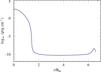
Figure 1: Density vs. radius for our $23\,M_{\odot}$ He model (cf. Table 1).

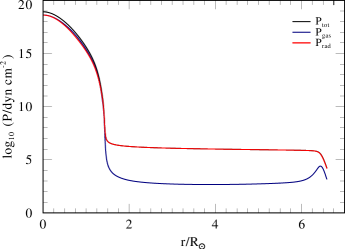
Figure 2: Pressure vs. radius. Gas pressure $P_{\rm gas}$, radiation pressure $P_{\rm rad}$, and total pressure $P_{\rm tot}=P_{\rm gas}+P_{\rm rad}$.

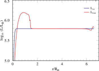
Figure 3: Total stellar luminosity $L(r)$, compared to the Eddington luminosity $L_{\rm Edd}=4\pi cGM/\kappa$.

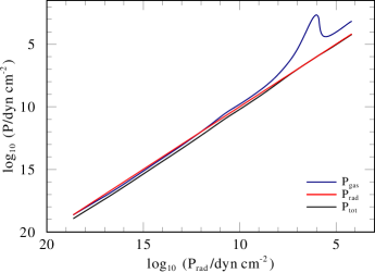
Figure 4: Stellar structure in the $P_{\rm rad}$–$P_{\rm gas}$ plane. Gas pressure $P_{\rm gas}$, radiation pressure $P_{\rm rad}$, and total pressure $P_{\rm tot}=P_{\rm gas}+P_{\rm rad}$ are plotted vs. $P_{\rm rad}$ throughout the whole star.

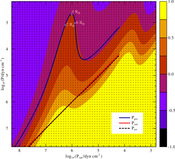
Figure 5: Envelope solution in the $P_{\rm rad}$–$P_{\rm gas}$ plane. The colors indicate the logarithm of the Eddington factor $\Gamma$, for given $P_{\rm rad}$ and $P_{\rm gas}$, according to the OPAL opacity tables (Iglesias & Rogers 1996), for our pure He model with $23\,M_{\odot}$. The envelope solution almost precisely follows a path with $\Gamma=1$. The radii of 2, 4, and $6\,R_{\odot}$ within the inflated envelope are indicated. Arrows indicate the slope of the solution, as expected from Eq. 12.

2.2 Stellar structure models with inflated envelopes

As a typical example for a model with an inflated envelope, we present a homogeneous stellar structure model for a 23 $M_{\odot}$ helium star with solar metallicity ($X=0$, $Y=0.98$, $Z=0.02$). In agreement with previous works by Ishii et al. (1999), and Petrovic et al. (2006), this model develops an extended low-density envelope, with a density inversion close to the surface (cf. Fig. 1). The star thus forms a shell around the actual stellar core, with a radius that is 3–4 times larger than the core radius.

Fig. 2 shows that the inflated region is dominated by radiation pressure. In this model, the gas pressure $P_{\rm gas}$ only accounts for a fraction of $\sim$ $4$$\cdot$$10^{-4}$ of the total pressure $P$. In contrast to this, $P_{\rm gas}$ and $P_{\rm rad}$ are roughly equal in the stellar core. The core is thus only fairly close to the Eddington limit, as reflected by an Eddington parameter of $\Gamma_{\rm e}\approx 0.4$ (cf. Table 1). Here $\Gamma_{\rm e}$ denotes the “classical” Eddington parameter, which is related to the Thomson opacity $\kappa_{\rm e}$ due to free electrons, i.e., $\Gamma_{\rm e}=\kappa_{\rm e}L_{\rm rad}/(4\pi cGM)$. The $\Gamma_{\rm e}$ given in Tables 1 and 2, are computed for a fully ionized plasma with a given hydrogen mass fraction $X$, and $L_{\rm rad}=L$. $\Gamma_{\rm e}$ then simplifies to

$$\log(\Gamma_{\rm e})=-4.813+\log(1+X)+\log(L/L_{\odot})-\log(M/M_{\odot}).$$ (6)

In contrast, the total Eddington factor $\Gamma=\kappa L_{\rm rad}/(4\pi cGM)$, which is related to the total opacity $\kappa$, approaches unity in the inflated zone. This is shown in Fig. 3, where we compare the total luminosity within our model with the Eddington luminosity $L_{\rm Edd}=4\pi cGM/\kappa$ (the condition $L_{\rm rad}=L_{\rm Edd}$ is thus equivalent to $\Gamma=1$). In Fig. 3 we can identify three zones within the star. In the inner, convective core, the total luminosity $L$ is larger than the Eddington luminosity $L_{\rm Edd}$. The main reason for this is that the energy transport is almost entirely convective, and thus $L_{\rm rad}$ is very low. Above this region follows the radiative envelope with $L<L_{\rm Edd}$. On top of this follows the inflated zone, where $L_{\rm Edd}$ almost equals $L$. $\Gamma$ is thus extremely close to one, almost throughout the complete outer envelope of the star. This is surprising, because $\Gamma$ is a function of the opacity $\kappa$, which is a strongly varying function of $\rho$, and $T$. The conditions in the inflated envelope thus demand for a mechanism that adjusts $\Gamma$ very precisely to one.

To achieve a large radial extension it is necessary that the density scale height $H$ is comparable to the stellar core radius $R_{\rm c}$. For our example model we have $R_{\rm c}/H=GM(1-\Gamma)/(a^{2}R_{\rm c})\approx 3$$\cdot$$10^{3}(1-\Gamma)$. From Fig. 2 we can infer that $(1-\Gamma)\approx P_{gas}/P\approx 4$$\cdot$$10^{-4}$ (cf. Eq. 15). Due to the low ratio of gas pressure to radiation pressure, $\Gamma$ is thus just close enough to one, to achieve a large radial extension.

A qualitative idea about the reason for the envelope inflation can be obtained from Fig. 4, where we plot the gas pressure $P_{\rm gas}$, and the total pressure $P$, vs. the radiation pressure $P_{\rm rad}$. This diagram is particularly useful, as for stars close to the Eddington limit, $P$ is of the same order of magnitude as $P_{\rm rad}$, i.e., in a logarithmic diagram the stellar structure just follows a straight line (in accordance with the Eddington standard model (Eddington 1918) for which $P_{\rm rad}/P=const.$ is adopted). For $P_{\rm gas}$ the situation is more complicated. In the stellar core, $P_{\rm gas}$ follows a similar relation as $P$. In the extended envelope, $P_{\rm gas}$ however drops significantly, and rises again after a certain minimum pressure $P_{\rm min}$ is reached. As demonstrated in Fig. 5, the region where $P_{\rm gas}$ drops corresponds precisely to the location of the Fe-opacity peak in the $P_{\rm rad}$–$P_{\rm gas}$ plane.

More explicitly, starting from the stellar core, the solution follows a straight line with $P_{\rm gas}/P_{\rm rad}=const.$ This naturally leads into a region in the $P_{\rm rad}$–$P_{\rm gas}$ plane, where the opacity $\kappa$ increases significantly, due to the presence of the Fe-opacity peak. When $\kappa$ reaches $\kappa_{\rm Edd}$, this leads to $\Gamma\rightarrow 1$. To avoid a super-Eddington situation, with $\Gamma>1$, either $L_{\rm rad}$, or $\kappa$ need to be reduced. $L_{\rm rad}$ could in principle be reduced by convection, however, in our case the involved densities turn out to be too low, i.e., convection is inefficient (cf. Sect. 3.5.4). The only possibility to reduce $\kappa$, is thus to lower the density. For this reason the density has to drop in our model, until the tip of the Fe-peak is reached (cf. Fig. 5). At the same time, however, this leads to a situation where $P_{\rm gas}\ll P_{\rm rad}$, and thus to $\Gamma\rightarrow 1$ (because, as already mentioned above $(1-\Gamma)\approx P_{\rm gas}/P$). This mechanism thus forces the solution to follow a path with $\Gamma=1$, i.e., with $\kappa(\rho,T)=\kappa_{\rm Edd}$.

As $P_{\rm rad}$, and $P_{\rm gas}$ are functions of $\rho$, and $T$, we can express $\kappa$ in the form $\kappa(P_{\rm gas},P_{\rm rad})$. This is actually done in Fig. 5, where the colors indicate $\kappa(P_{\rm gas},P_{\rm rad})/\kappa_{\rm Edd}$ on a logarithmic scale, as obtained from the OPAL opacity tables (Iglesias & Rogers 1996). In this plot we can see that the solution within the low-density zone is completely dominated by the topology of the opacity $\kappa$, i.e., by material properties. As soon as the solution reaches low densities close to the Fe-opacity peak, it just follows a path with $\Gamma=1$, until a minimum density $\rho_{\rm min}$ is reached. This minimum is located at the tip of the Fe-opacity peak, typically at $P_{\rm rad}\approx 10^{6}\,{\rm dyn\,cm}^{-2}$, corresponding to a temperature of $\sim$ 150 kK. After the opacity peak is passed, the solution still follows $\Gamma=1$, but now with increasing $P_{\rm gas}$, leading to a density inversion.

To maintain the described envelope inflation, it is thus necessary that 1) the star is close enough to the Eddington limit, so that $\Gamma\rightarrow 1$, and 2) convection is inefficient. If the envelope inflation occurs, its properties are determined by the topology of the Fe-opacity peak in the $P_{\rm rad}$–$P_{\rm gas}$ plane, i.e., by material properties. In Sect. 3, this will help us to find an analytical description of the inflation effect. It also implies a dependence on material properties like the metallicity $Z$, as discussed by Ishii et al. (1999), and Petrovic et al. (2006). In Sect. 2.4, we will discuss an additional important effect, namely the influence of density inhomogeneities within the inflated zone, which is based on a similar principle.

2.3 A grid of homogeneous stellar structure models with envelope inflation

Table 1: Model parameters for pure helium models.

$M_{\star}$	$L_{\star}$	$\Gamma_{\rm e}$	$\log(T_{\rm c})$	$\log(T_{\star})$	$R_{\rm c}$	$R_{\rm e}$	$R_{\star}$	$\Delta R$	$\Delta R$	$\Delta M$	$\rho_{\rm min}$	$f_{\rho}$	$Q$	$W_{c}$	$W_{e}$	$P_{\rm e}$
$[M_{\odot}]$	$[L_{\odot}]$		$[{\rm K}]$	$[{\rm K}]$	$[R_{\odot}]$	[$R_{\odot}$]	$[R_{\odot}]$	$[R_{\rm c}]$	$[R_{\rm e}]$	$[M_{\odot}]$	$[\frac{\rm g}{{\rm cm}^{3}}]$					$[\frac{\rm dyn}{{\rm cm}^{2}}]$
$X=0.00$, $D=1$
23.7	5.813	0.414	5.11	4.61	1.6	14.6	16.5	7.99	0.89	$1.9$$\cdot$$10^{-6}$	$4.4$$\cdot$$10^{-11}$	2.4	30.50	0.89	7.99	$6.8$$\cdot$$10^{5}$
23.5	5.807	0.412	5.10	4.68	1.7	10.5	11.4	5.35	0.84	$4.6$$\cdot$$10^{-7}$	$4.6$$\cdot$$10^{-11}$	2.1	25.27	0.84	5.35	$6.8$$\cdot$$10^{5}$
23.0	5.792	0.406	5.10	4.80	1.6	6.3	6.6	2.88	0.74	$5.7$$\cdot$$10^{-8}$	$5.4$$\cdot$$10^{-11}$	2.1	21.90	0.74	2.88	$6.9$$\cdot$$10^{5}$
22.0	5.761	0.396	5.11	4.92	1.6	3.6	3.7	1.35	0.57	$6.6$$\cdot$$10^{-9}$	$7.3$$\cdot$$10^{-11}$	2.0	16.61	0.57	1.35	$7.1$$\cdot$$10^{5}$
21.0	5.729	0.385	5.11	4.98	1.5	2.7	2.7	0.79	0.44	$2.0$$\cdot$$10^{-9}$	$9.9$$\cdot$$10^{-11}$	2.0	12.69	0.44	0.79	$7.1$$\cdot$$10^{5}$
20.0	5.694	0.373	5.11	5.01	1.4	2.2	2.2	0.52	0.34	$9.6$$\cdot$$10^{-10}$	$1.4$$\cdot$$10^{-10}$	2.1	10.28	0.34	0.52	$7.4$$\cdot$$10^{5}$
19.0	5.658	0.361	5.11	5.04	1.4	1.9	1.9	0.36	0.26	$5.3$$\cdot$$10^{-10}$	$1.9$$\cdot$$10^{-10}$	2.1	7.80	0.26	0.36	$6.9$$\cdot$$10^{5}$
18.0	5.618	0.348	5.11	5.06	1.3	1.6	1.7	0.25	0.20	$3.6$$\cdot$$10^{-10}$	$2.7$$\cdot$$10^{-10}$	2.1	5.90	0.20	0.25	$6.9$$\cdot$$10^{5}$
17.0	5.576	0.335	5.11	5.07	1.3	1.5	1.5	0.19	0.16	$2.7$$\cdot$$10^{-10}$	$3.9$$\cdot$$10^{-10}$	2.3	4.81	0.16	0.19	$7.0$$\cdot$$10^{5}$
16.0	5.531	0.320	5.10	5.07	1.2	1.4	1.4	0.14	0.12	$2.1$$\cdot$$10^{-10}$	$5.5$$\cdot$$10^{-10}$	2.3	3.76	0.12	0.14	$6.8$$\cdot$$10^{5}$
15.0	5.482	0.305	5.10	5.08	1.2	–	1.3	–	–	–	–	–	3.10	–	–	–
14.0	5.429	0.289	5.10	5.08	1.1	–	1.2	–	–	–	–	–	2.31	–	–	–
12.0	5.307	0.255	5.09	5.07	1.0	–	1.1	–	–	–	–	–	1.27	–	–	–
10.0	5.155	0.216	5.07	5.06	0.9	–	0.9	–	–	–	–	–	0.69	–	–	–
8.0	4.959	0.172	5.05	5.04	0.8	–	0.8	–	–	–	–	–	0.36	–	–	–
$X=0.00$, $D=4$
18.5	5.638	0.355	5.10	4.69	1.4	8.1	9.2	4.82	0.83	$2.0$$\cdot$$10^{-7}$	$5.8$$\cdot$$10^{-11}$	1.9	21.09	0.83	4.82	$6.4$$\cdot$$10^{5}$
18.0	5.618	0.348	5.10	4.81	1.4	4.8	5.1	2.51	0.72	$2.2$$\cdot$$10^{-8}$	$6.9$$\cdot$$10^{-11}$	1.9	18.09	0.72	2.51	$6.3$$\cdot$$10^{5}$
17.0	5.576	0.335	5.10	4.93	1.3	2.8	2.9	1.14	0.53	$2.6$$\cdot$$10^{-9}$	$9.8$$\cdot$$10^{-11}$	1.9	13.21	0.53	1.14	$6.2$$\cdot$$10^{5}$
16.0	5.531	0.320	5.10	4.98	1.2	2.0	2.1	0.65	0.40	$7.7$$\cdot$$10^{-10}$	$1.4$$\cdot$$10^{-10}$	1.9	9.86	0.40	0.65	$5.9$$\cdot$$10^{5}$
15.0	5.482	0.305	5.10	5.02	1.2	1.7	1.7	0.42	0.29	$3.6$$\cdot$$10^{-10}$	$2.0$$\cdot$$10^{-10}$	2.0	7.44	0.29	0.42	$5.6$$\cdot$$10^{5}$
14.0	5.429	0.289	5.09	5.04	1.1	–	1.5	–	–	–	–	–	6.14	–	–	–
13.0	5.371	0.273	5.09	5.05	1.1	–	1.3	–	–	–	–	–	4.45	–	–	–
12.0	5.307	0.255	5.08	5.05	1.0	–	1.2	–	–	–	–	–	3.01	–	–	–
10.0	5.155	0.216	5.07	5.05	0.9	–	1.0	–	–	–	–	–	1.43	–	–	–
8.0	4.959	0.172	5.05	5.04	0.8	–	0.8	–	–	–	–	–	0.69	–	–	–
$X=0.00$, $D=10$
15.5	5.507	0.313	5.10	4.66	1.2	7.3	8.9	5.10	0.84	$1.5$$\cdot$$10^{-7}$	$6.7$$\cdot$$10^{-11}$	2.2	23.29	0.84	5.10	$5.6$$\cdot$$10^{5}$
15.0	5.482	0.305	5.09	4.80	1.2	4.2	4.6	2.52	0.72	$1.3$$\cdot$$10^{-8}$	$8.1$$\cdot$$10^{-11}$	2.0	18.22	0.72	2.52	$5.4$$\cdot$$10^{5}$
14.0	5.429	0.289	5.09	4.92	1.1	–	2.5	–	–	–	–	–	14.52	–	–	–
13.0	5.371	0.273	5.09	4.98	1.1	–	1.8	–	–	–	–	–	10.24	–	–	–
12.0	5.307	0.255	5.08	5.01	1.0	–	1.5	–	–	–	–	–	6.97	–	–	–
10.0	5.155	0.216	5.07	5.03	0.9	–	1.1	–	–	–	–	–	3.07	–	–	–
8.0	4.959	0.172	5.05	5.03	0.8	–	0.9	–	–	–	–	–	1.33	–	–	–
$X=0.00$, $D=16$
14.0	5.429	0.289	5.08	4.65	1.2	5.9	8.5	3.97	0.80	$1.0$$\cdot$$10^{-7}$	$7.4$$\cdot$$10^{-11}$	1.5	14.59	0.80	3.97	$4.7$$\cdot$$10^{5}$
13.5	5.401	0.281	5.08	4.80	1.2	3.5	4.3	1.97	0.66	$8.1$$\cdot$$10^{-8}$	$8.9$$\cdot$$10^{-11}$	1.4	10.99	0.66	1.97	$4.0$$\cdot$$10^{5}$
13.0	5.371	0.273	4.88	4.87	2.8	–	3.0	–	–	–	–	–	0.56	–	–	–
12.0	5.307	0.255	5.08	4.95	1.0	–	1.9	–	–	–	–	–	10.49	–	–	–
10.0	5.155	0.216	5.07	5.01	0.9	–	1.2	–	–	–	–	–	4.75	–	–	–
8.0	4.959	0.172	5.05	5.02	0.8	–	0.9	–	–	–	–	–	2.06	–	–	–

Table 2: Model parameters for chemically-homogeneous stars containing hydrogen.

$M_{\star}$	$L_{\star}$	$\Gamma_{\rm e}$	$\log(T_{\rm c})$	$\log(T_{\star})$	$R_{\rm c}$	$R_{\rm e}$	$R_{\star}$	$\Delta R$	$\Delta R$	$\Delta M$	$\rho_{\rm min}$	$f_{\rho}$	$Q$	$W_{c}$	$W_{e}$	$P_{\rm e}$
$[M_{\odot}]$	$[L_{\odot}]$		$[{\rm K}]$	$[{\rm K}]$	$[R_{\odot}]$	[$R_{\odot}$]	$[R_{\odot}]$	$[R_{\rm c}]$	$[R_{\rm e}]$	$[M_{\odot}]$	$[\frac{\rm g}{{\rm cm}^{3}}]$					$[\frac{\rm dyn}{{\rm cm}^{2}}]$
$X=0.70$, $D=1$
155.0	6.418	0.435	4.70	4.20	21.3	163.3	217.6	6.68	0.87	$7.1$$\cdot$$10^{-3}$	$1.0$$\cdot$$10^{-10}$	2.3	14.27	0.87	6.68	$8.6$$\cdot$$10^{5}$
150.0	6.397	0.427	4.70	4.38	20.7	80.0	90.6	2.86	0.74	$3.2$$\cdot$$10^{-4}$	$1.3$$\cdot$$10^{-10}$	2.2	11.65	0.74	2.86	$8.6$$\cdot$$10^{5}$
145.0	6.375	0.420	4.71	4.47	19.9	53.6	58.0	1.69	0.63	$6.2$$\cdot$$10^{-5}$	$1.5$$\cdot$$10^{-10}$	2.2	10.08	0.63	1.69	$8.6$$\cdot$$10^{5}$
140.0	6.351	0.412	4.71	4.53	19.2	41.1	43.6	1.14	0.53	$2.2$$\cdot$$10^{-5}$	$1.9$$\cdot$$10^{-10}$	2.2	8.62	0.53	1.14	$8.5$$\cdot$$10^{5}$
130.0	6.301	0.396	4.71	4.60	17.9	29.2	30.2	0.63	0.39	$5.5$$\cdot$$10^{-6}$	$2.9$$\cdot$$10^{-10}$	2.3	6.45	0.39	0.63	$8.0$$\cdot$$10^{5}$
120.0	6.247	0.378	4.71	4.63	16.7	–	23.9	–	–	–	–	–	5.46	–	–	–
110.0	6.186	0.359	4.71	4.66	15.7	–	20.2	–	–	–	–	–	3.77	–	–	–
100.0	6.118	0.337	4.71	4.67	14.6	–	17.6	–	–	–	–	–	2.58	–	–	–
90.0	6.041	0.314	4.70	4.67	13.7	–	15.7	–	–	–	–	–	1.76	–	–	–
80.0	5.952	0.288	4.70	4.67	12.7	–	14.1	–	–	–	–	–	1.20	–	–	–
70.0	5.848	0.259	4.69	4.67	11.7	–	12.7	–	–	–	–	–	0.81	–	–	–
60.0	5.724	0.227	4.68	4.66	10.7	–	11.5	–	–	–	–	–	0.55	–	–	–
50.0	5.569	0.191	4.66	4.65	9.6	–	10.2	–	–	–	–	–	0.36	–	–	–
40.0	5.368	0.150	4.63	4.63	8.9	–	8.9	–	–	–	–	–	0.10	–	–	–
30.0	5.087	0.105	4.59	4.59	7.6	–	7.6	–	–	–	–	–	0.09	–	–	–
20.0	4.647	0.057	4.53	4.53	6.0	–	6.1	–	–	–	–	–	0.09	–	–	–
$X=0.40$, $D=1$
80.0	6.179	0.400	4.73	4.29	14.3	86.8	106.6	5.07	0.84	$8.9$$\cdot$$10^{-4}$	$1.6$$\cdot$$10^{-10}$	2.6	12.21	0.84	5.07	$8.1$$\cdot$$10^{5}$
75.0	6.135	0.385	4.73	4.50	13.4	35.7	38.4	1.66	0.62	$2.2$$\cdot$$10^{-5}$	$2.3$$\cdot$$10^{-10}$	2.7	9.46	0.62	1.66	$7.7$$\cdot$$10^{5}$
70.0	6.088	0.370	4.72	4.59	13.1	23.8	24.8	0.82	0.45	$4.3$$\cdot$$10^{-6}$	$3.4$$\cdot$$10^{-10}$	2.3	5.43	0.45	0.82	$7.6$$\cdot$$10^{5}$
65.0	6.036	0.354	4.73	4.63	12.3	–	19.0	–	–	–	–	–	4.73	–	–	–
60.0	5.979	0.336	4.73	4.66	11.5	–	15.7	–	–	–	–	–	3.38	–	–	–
50.0	5.844	0.296	4.72	4.68	10.1	–	12.0	–	–	–	–	–	1.69	–	–	–
40.0	5.671	0.248	4.71	4.68	8.8	–	9.8	–	–	–	–	–	0.83	–	–	–
30.0	5.431	0.190	4.68	4.67	7.4	–	8.0	–	–	–	–	–	0.39	–	–	–
20.0	5.054	0.120	4.63	4.63	6.2	–	6.2	–	–	–	–	–	0.09	–	–	–
15.0	4.756	0.080	4.59	4.59	5.3	–	5.3	–	–	–	–	–	0.09	–	–	–
$X=0.20$, $D=1$
46.0	5.975	0.372	4.74	4.37	10.7	50.9	59.5	3.75	0.79	$1.6$$\cdot$$10^{-4}$	$2.3$$\cdot$$10^{-10}$	2.4	7.97	0.79	3.75	$7.8$$\cdot$$10^{5}$
45.0	5.960	0.367	4.74	4.45	10.7	36.7	40.8	2.43	0.71	$4.1$$\cdot$$10^{-5}$	$2.6$$\cdot$$10^{-10}$	2.2	6.56	0.71	2.43	$7.7$$\cdot$$10^{5}$
44.0	5.944	0.362	4.74	4.50	10.4	29.0	31.5	1.78	0.64	$1.6$$\cdot$$10^{-5}$	$2.9$$\cdot$$10^{-10}$	2.2	6.00	0.64	1.78	$7.7$$\cdot$$10^{5}$
42.0	5.911	0.352	4.74	4.57	10.0	20.9	22.1	1.09	0.52	$4.2$$\cdot$$10^{-6}$	$3.8$$\cdot$$10^{-10}$	2.2	4.86	0.52	1.09	$7.5$$\cdot$$10^{5}$
40.0	5.877	0.341	4.74	4.61	9.6	16.8	17.4	0.75	0.43	$1.7$$\cdot$$10^{-6}$	$4.9$$\cdot$$10^{-10}$	2.3	4.10	0.43	0.75	$7.0$$\cdot$$10^{5}$
35.0	5.780	0.312	4.74	4.67	8.6	–	11.9	–	–	–	–	–	2.73	–	–	–
30.0	5.664	0.279	4.73	4.69	7.7	–	9.4	–	–	–	–	–	1.53	–	–	–
25.0	5.520	0.240	4.72	4.70	6.8	–	7.8	–	–	–	–	–	0.84	–	–	–
20.0	5.334	0.195	4.71	4.69	6.0	–	6.5	–	–	–	–	–	0.45	–	–	–
15.0	5.073	0.143	4.68	4.66	5.1	–	5.4	–	–	–	–	–	0.23	–	–	–
10.0	4.664	0.084	4.61	4.61	4.3	–	4.3	–	–	–	–	–	0.09	–	–	–
$X=0.36$, $D=1$ (AG Car)
73.0	6.149	0.397	4.72	4.23	14.3	104.3	136.8	6.30	0.86	$2.2$$\cdot$$10^{-3}$	$1.6$$\cdot$$10^{-10}$	2.2	9.68	0.86	6.30	$8.0$$\cdot$$10^{5}$
70.0	6.120	0.387	4.72	4.44	13.8	46.1	51.3	2.36	0.70	$6.8$$\cdot$$10^{-5}$	$2.0$$\cdot$$10^{-10}$	2.2	7.69	0.70	2.36	$8.0$$\cdot$$10^{5}$
65.0	6.069	0.371	4.73	4.56	12.7	25.6	26.9	1.02	0.50	$6.3$$\cdot$$10^{-6}$	$3.1$$\cdot$$10^{-10}$	2.3	5.89	0.50	1.02	$7.7$$\cdot$$10^{5}$
60.0	6.013	0.353	4.73	4.62	11.8	–	19.2	–	–	–	–	–	4.90	–	–	–

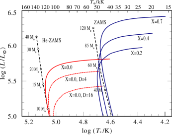
Figure 6: HR diagram for pure helium models (red), and models containing hydrogen (blue).

To assess the effect of the envelope inflation in the HR diagram, we have computed a grid of homogeneous stellar structure models with hydrogen mass fractions $X=0.0$, 0.2, 0.4, and 0.7, that covers a luminosity range between $\log(L/L_{\odot})=5.0$, and 6.5. The results are compiled in Tables 1 and 2. In Fig. 6, we show the position of our models in the HR diagram, together with theoretical zero-age main sequences (ZAMS) that do not take the inflation effect into account.

At low luminosities, our He-burning models (with $X=0.0$) closely resemble the He-ZAMS from Langer (1989b), and our H-burning models ($X=0.2$–0.7) the ZAMS from Schaller et al. (1992). Towards higher luminosities, our models develop inflated envelopes, i.e., they show lower $T_{\star}$. With increasing luminosity, $T_{\star}$ decreases rapidly until, above a certain luminosity, we do not find static solutions anymore. The reason for the occurrence of this important limit will be explained in Sect. 3.2.

In our present models, the envelope inflation sets in for Eddington factors $\Gamma_{\rm e}$ between 0.3 ($X=0.0$), and 0.4 ($X=0.7$), i.e., within a relatively narrow range. The fact that it sets in earlier for H-deficient stars is a consequence of the fact that the $L/M$ ratios of these objects are higher (although $\kappa_{\rm e}$ is lower for lower H abundances). In Sects. 3.2, & 3.3 we will show that this behavior, as well as the described upper luminosity limit, are a consequence of the strength, and shape of the Fe-opacity peak in the $P_{\rm rad}$–$P_{\rm gas}$ plane.

2.4 The influence of density inhomogeneities

For our pure He models in Table 1, the described envelope extension starts at luminosities of $\log(L/L_{\odot})\approx 5.5$, and fully develops for $\log(L/L_{\odot})\approx 5.8$ (cf. Fig. 6). As we will discuss in Sect. 4.1, the largest part of the Galactic H-free Wolf-Rayet stars, however, seems to show inflated envelopes for luminosities just below this value. In the following we will show that the inflation in this parameter range can be explained by density inhomogeneities. Such inhomogeneities are expected to arise in the outer envelopes of WR stars, e.g. due to strange-mode instabilities (Glatzel & Kaltschmidt 2002; Glatzel 2008).

If material is inhomogeneous, or clumped, the density within clumps is larger than the mean density. As a result, the opacity $\kappa$ has to be evaluated for an increased density, instead of the mean density (note that $\kappa$ denotes the mass absorption coefficient in ${\rm cm}^{2}/{\rm g}$). Here we assume a constant clumping factor $D$ within the inflated envelope, and evaluate $\kappa(\rho,T)$ for the enhanced density $D\times\rho$, instead of the mean density $\rho$. This is equivalent to assuming a medium with clumps of a constant density $D\times\rho$, and an inter-clump medium which is void. In this picture the clumps would thus only fill a fraction $f=1/D$ of the total volume. The same definition of clumping factors $D$, and filling factors $f$ is commonly used for the modeling of inhomogeneous stellar winds (e.g. Hamann & Koesterke 1998).

In the clumping approximation used here, it is assumed that no radiative flux gets lost in between clumps, e.g. by shadowing/porosity effects. Such a situation could be achieved by optically thin clumps, or by a clump geometry (such as large shells, or pancakes) that is not sensitive to shadowing effects.

Following our argumentation from the previous section, large envelope extensions, i.e., large scale heights $H$, are reached for Eddington factors $\Gamma$ that are very close to one. We have shown that this is achieved for the low values of $P_{\rm gas}$ at the tip of the Fe-opacity peak, as $P_{\rm gas}/P\approx(1-\Gamma)$. By the assumption of clumping, the opacity peak is shifted towards even lower mean densities, i.e., towards lower (mean) values of $P_{\rm gas}$. In this way, the envelope inflation is further enhanced (a more concise explanation of this effect is given in Sect. 3,  Eqs. 19, 20  29).

In Fig. 6 we show He-ZAMS models that are computed with clumping factors $D=4$, and $D=16$. As expected, the envelope extension occurs much earlier in these models. In Sect. 4.1 we will show that these models cover the observed HR diagram (HRD) positions of the Galactic H-free WR stars, i.e., we can explain the observed temperatures of these objects with moderate clumping factors. The adopted values for $D$ are in notable agreement with spectroscopically determined clumping factors for the winds of WR stars, e.g. by Hamann & Koesterke (1998).

3 Analytical description of the envelope inflation

In the previous section we have shown that the properties of inflated envelopes are chiefly determined by the fact that the solution has to follow a path with $\Gamma=1$ in the $P_{\rm rad}$–$P_{\rm gas}$ plane (cf. Fig. 5). In the following we elaborate on this, and derive an analytical description of this process. As we concentrate on the physics of the inflated envelopes alone, the resulting relations do not depend on the internal structure of the star, i.e., they are generally applicable to stars with given (observed) parameters. In Sect. 3.1, we start with the equations describing the envelope structure. In Sect. 3.2 we derive analytical expressions for the radial extension of the envelope $\Delta R$, and in Sect. 3.3 we present a recipe to estimate $\Delta R$ based on observed/adopted stellar parameters. Furthermore, we derive an estimate for the mass of the surrounding shell, $\Delta M$, in Sect. 3.4. Finally, we discuss in Sect. 3.5, to which extent the inflation effect may be affected by model assumptions.

3.1 Inflated low-density envelopes near the Eddington limit

In this section we concentrate on the physics of the outermost stellar envelope, where $m=M$, and $L=const.$ With these assumptions, we eliminate two equations from the stellar structure equations (Eqs. 1–4), so that only the equation of hydrostatic equilibrium (Eq. 1), and the energy transport equation (Eq. 4) are left.

In Sect. 2.2 we concluded, that two conditions are mandatory to maintain an inflated envelope. 1) the star needs to be close enough to the Eddington limit, so that $\Gamma=1$ can be reached, and 2) convective energy transport needs to be inefficient. Under condition 2) (the validity of this condition is discussed in Sect. 3.5.4), the energy transport equation (Eq. 4) becomes purely radiative, i.e., $L=L_{\rm rad}$, and $\nabla=\nabla_{\rm rad}$, with

$$\nabla_{\rm rad}=\frac{3}{16\pi ac}\frac{P\kappa}{T^{4}}\frac{L}{GM}.$$ (7)

After substituting Eq. 1, and Eq. 2 in Eq. 4, we thus obtain the energy transport equation in the form

$$\frac{\partial T}{\partial r}=-\frac{3}{4aT^{3}}\frac{\kappa\rho L}{4\pi r^{2}c}.$$ (8)

If this relation is written in terms of $P_{\rm rad}=(a/3)T^{4}$ we obtain

$$\frac{\partial P_{\rm rad}}{\partial r}=\frac{4aT^{3}}{3}\frac{\partial T}{\partial r}=-\frac{\kappa\rho L}{4\pi r^{2}c}=-\rho g_{\rm rad},$$ (9)

for the (outward directed) radiative acceleration $g_{\rm rad}$. Together with the equation of hydrostatic equilibrium

$$\frac{\partial P}{\partial r}=\frac{\partial(P_{\rm gas}+P_{\rm rad})}{\partial r}=-\frac{GM\rho}{r^{2}}=-\rho g,$$ (10)

we obtain by division of Eq. 10 and Eq. 9

$$\frac{\partial P}{\partial P_{\rm rad}}=\frac{\partial P_{\rm gas}}{\partial P_{\rm rad}}+1=\frac{g}{g_{\rm rad}}=\frac{1}{\Gamma},$$ (11)

or

$$\frac{\partial P_{\rm gas}}{\partial P_{\rm rad}}=\frac{1}{\Gamma}-1.$$ (12)

Notably, ${\partial P_{\rm gas}}/{\partial P_{\rm rad}}$ depends only on the Eddington factor $\Gamma$, i.e., via $\Gamma/\Gamma_{\rm e}=\kappa/\kappa_{\rm e}$ on $\Gamma_{\rm e}$, and $\kappa$. This is in line with our previous finding that the envelope inflation is fully determined by the classical Eddington factor $\Gamma_{\rm e}$ (as given by Eq. 6), which is a function of stellar parameters, and $\kappa$, which depends on material properties.

In Fig. 5 we compare our numerical solution from Sect. 2.2 (blue line) with the slopes ${\partial P_{\rm rad}}/{\partial P_{\rm gas}}$ (black arrows) following from Eq. 12, in the $P_{\rm rad}$–$P_{\rm gas}$ plane. The background colors indicate the value of $\Gamma=\Gamma_{\rm e}(\kappa/\kappa_{\rm e})$ for our model, where $\kappa$ has been extracted from the OPAL opacity tables (Iglesias & Rogers 1996).

According to Eq. 12, the point at which the envelope solution crosses the Eddington limit, i.e. where $\Gamma=1$, needs to be an extremum in $P_{\rm gas}$. Fig. 5 nicely shows, that our numerical solution indeed approaches the Eddington limit, and crosses it at the point of the lowest possible gas pressure. If the Eddington limit would be crossed earlier, at a higher density, the gas pressure had to increase so fast, that extremely high densities would be required at the outer boundary. The only way to reach reasonably low temperatures, and densities at the outer boundary, thus leads around the Fe-opacity peak, via a low gas pressure, i.e., via low densities. The formation of a low-density envelope with a density inversion is thus a natural consequence of the topology of the Fe opacity peak in the $P_{\rm rad}$–$P_{\rm gas}$ plane, in combination with Eq. 12.

For the example in Fig. 5, we find that $P_{\rm gas}/P_{\rm rad}\approx 4$$\cdot$$10^{-4}$ at the tip of the Fe-opacity peak. In Sect. 2.2 we already discussed that this implies that $\Gamma\rightarrow 1$, as $P_{\rm gas}/P\approx(1-\Gamma)$. This relation follows from Eq. 11, if we assume a slowly changing ratio $P_{\rm rad}/P$. In this case we have $\partial(\ln P_{\rm rad})/\partial(\ln P)\approx 1$ (cf.  Fig. 4). It thus follows that

$$\frac{\partial(\ln P_{\rm rad})}{\partial(\ln P)}=\frac{P}{P_{\rm rad}}\frac{\partial P_{\rm rad}}{\partial P}=\frac{P}{P_{\rm rad}}\,\Gamma\approx 1,$$ (13)

which leads to

$$\frac{P_{\rm rad}}{P}\approx\Gamma,$$ (14)

or

$$\frac{P_{\rm gas}}{P}=\frac{P_{\rm gas}}{P_{\rm gas}+P_{\rm rad}}\approx(1-\Gamma).$$ (15)

As discussed in Sect. 2.2, this small value of $(1-\Gamma)$ leads to a density scale height of the order of the stellar radius, i.e., to an envelope inflation.

The occurrence of an envelope inflation is thus intimately connected to the fact that $P_{\rm gas}\ll P_{\rm rad}$ at the tip of the Fe-opacity peak. As noted earlier, the location of this point in the ${P_{\rm rad}}$–${P_{\rm gas}}$ plane is only determined by the topology of the opacity peak, i.e., by material properties. In the following we will take advantage of this fact, to obtain analytical estimates of the radial envelope extension $\Delta R$.

3.2 Computation of the radial extension $\Delta R$

To compute the radial extension $\Delta R$, we integrate Eq. 9 and Eq. 10 from the outer boundary of the inflated zone, at the “envelope radius” $R_{\rm e}$, to the inner boundary, at the “core radius” $R_{\rm c}$. As this integration is performed within the inflated zone, where $P=P_{\rm rad}$, and $\kappa=\kappa_{\rm Edd}$, Eqs. 9 and 10 degenerate to one equation, that describes the change of $P_{\rm rad}$, and thus also the change of the temperature, in hydrostatic equilibrium.

$$\frac{\partial P_{\rm rad}}{\partial r}=-\frac{\kappa_{\rm Edd}\rho L}{4\pi r^{2}c}=-\frac{GM\rho}{r^{2}},$$ (16)

or

$$\frac{{\rm d}P_{\rm rad}}{\rho}=GM\,{\rm d}\frac{1}{r}.$$ (17)

The integration is performed from $R_{\rm e}$, where $P\equiv P_{\rm e}$, to $R_{\rm c}$, where $P\equiv P_{\rm c}$, leading to

$$\frac{R_{\rm c}}{GM}\int_{P_{\rm e}}^{P_{\rm c}}\frac{{\rm d}P_{\rm rad}}{\rho}=1-\frac{R_{\rm c}}{R_{\rm e}}.$$ (18)

The left hand side of this equation can be written in the form

$$W_{\rm c}\equiv\frac{R_{\rm c}}{GM}\frac{\Delta P}{\bar{\rho}},$$ (19)

where $\Delta P=P_{\rm c}-P_{\rm e}$, and $1/\bar{\rho}$ is the mean of $1/\rho$ with respect to $P_{\rm rad}$. In Sect. 3.3 we will show that $\Delta P$, and $\bar{\rho}$ can be estimated alone on the basis of opacity tables. For given $W_{\rm c}$, the radial envelope extension can then be computed from Eq. 18, which becomes

$$\frac{R_{e}}{R_{c}}=\frac{1}{1-W_{\rm c}}=1+W_{\rm e},$$ (20)

where the latter equality uses a definition of $W$ in terms of the observable, outer-envelope radius $R_{\rm e}$

$$W_{\rm e}\equiv\frac{R_{\rm e}}{GM}\frac{\Delta P}{\bar{\rho}}.$$ (21)

The expression for the radial extension $\Delta R=R_{\rm e}-R_{\rm c}$ for given $W_{\rm c}$, or $W_{\rm e}$ follows directly from Eq. 20

$$\frac{\Delta R}{R_{\rm c}}=\frac{1}{1-W_{\rm c}}-1,$$ (22)

$$\frac{\Delta R}{R_{\rm e}}=1-\frac{1}{1+W_{\rm e}}.$$ (23)

For the $W_{\rm c}$, and $W_{\rm e}$ as determined from our models (Tables 1 and 2) these relations are fulfilled very precisely.

The parameters $W_{\rm c/e}$ are of essential importance for the inflation effect. As $u=3P/\rho$ in a radiation dominated gas (where $u$ denotes the specific energy per volume), $\Delta P/\bar{\rho}$ is related to the specific energy per gram of material within the inflated zone. According to Eq. 18, it denotes the increase of the specific energy, from the outer to the inner edge of the inflated envelope, divided by 3. The parameters $W_{\rm c/e}$ indicate the ratio between this energy increase, and the gravitational energy per gram of material, at $R_{\rm c/e}$.

Notably, Eq. 20 imposes an instability limit for $W_{\rm c}\rightarrow 1$, for which $R_{\rm e}\rightarrow\infty$. This limit coincides with the limit that we have described in Sect. 2.3, where we found that no hydrostatic solutions exist, if certain luminosities are exceeded. Stable solutions only exist for $W_{\rm c}<1$, which is equivalent to

$$\frac{\Delta P}{\bar{\rho}}<\frac{GM}{R_{\rm c}}.$$ (24)

As $\Delta P/\bar{\rho}$ is largely fixed by material properties, Eq. 24 imposes a limit on the gravitational energy at the core radius $R_{\rm c}$. If the gravitational energy becomes too small (i.e., $R_{\rm c}$ becomes too large), the stellar envelope becomes energetically unbound, and there exists no hydrostatic envelope solution. This limit might be of profound importance for the occurrence of instabilities close to the Eddington limit, as observed, e.g. for LBVs (cf. Sec. 4.2).

The occurrence of the envelope inflation is thus mainly due to the fact that the Fe-opacity peak forces the envelope to low densities $\rho$, while the temperature of the opacity peak is fixed, i.e., $u=const$. This leads to a very high specific energy $u/\rho$, i.e., the envelope becomes less gravitationally bound.

3.3 A recipe to compute $\Delta R$

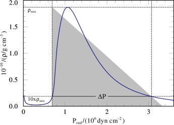
Figure 7: Plot of $1/\rho$ vs. $P_{\rm rad}$. The dashed horizontal lines indicate $1/\rho_{\rm min}$, and $1/(10\,\rho_{\rm min})$. The intersections of the latter with the envelope solution represent boundary pressure $P_{\rm c}$, and $P_{\rm e}$, as indicated by vertical dashed lines. The grey shaded area illustrates that the integral $\int\,\mbox{d}P/\rho\approx\Delta P/(2\rho_{\rm min})$.

The remaining step for the computation of $\Delta R$ is to obtain estimates of the parameter W (Eqs. 19, 21), which depends on the ratio $M/R$ (where $R$ denotes either $R_{\rm c}$, or $R_{\rm e}$), and the ratio $\Delta P/\bar{\rho}$. While $M$, and $R$ are given stellar parameters, $\Delta P/\bar{\rho}$ needs to be determined from opacity tables.

Based on Eqs. 18, 19 we have

$$\frac{\Delta P}{\bar{\rho}}=\int_{P_{\rm e}}^{P_{\rm c}}\frac{{\rm d}P_{\rm rad}}{\rho}.$$ (25)

In Fig. 7 we illustrate that, due to the topology of the Fe-opacity peak, the integral on the right hand side is roughly equal to $\Delta P/(2\rho_{\rm min})$, i.e.,

$$W=\frac{R}{GM}\frac{\Delta P}{\bar{\rho}}=\frac{R}{GM}\frac{\Delta P}{f_{\rho}\rho_{\rm min}},$$ (26)

with $f_{\rho}\approx 2$. Numerically obtained values for $f_{\rho}$ from our model computations confirm this value (cf. Table 1 and 2). $W$ can thus be computed on the basis of $\Delta P=P_{\rm c}-P_{\rm e}$, and $\rho_{\rm min}$.

To extract these values from the opacity tables, we make use the fact that the envelope solution follows almost precisely a path with $\Gamma=1$, i.e., a path with $\kappa=\kappa_{\rm Edd}$ in the $P_{\rm rad}$–$P_{\rm gas}$ plane. From this path we extract the minimum gas pressure $P_{\rm min}$, at the tip of the Fe-opacity peak (cf. Fig. 5). We use the density at this point as our reference density $\rho_{\rm min}$. For given $P_{\rm min}$, we define the boundaries of the inflated envelope as the two adjacent points on the path with $\kappa=\kappa_{\rm Edd}$, where $P_{\rm gas}=f_{P}\cdot P_{\rm min}$ (in this work we use $f_{P}=10$). The radiation pressure at these two points gives us $P_{\rm c}$, and $P_{\rm e}$. Our choice of $f_{P}=10$ has a moderate influence on the resulting values, will however not change the overall results.

The procedure described above thus provides $\rho_{\rm min}$, and $\Delta P=P_{\rm c}-P_{\rm e}$ for given $\kappa_{\rm Edd}$, or $\Gamma_{\rm e}$ (note that $\Gamma_{\rm e}(\kappa_{\rm Edd}/\kappa_{\rm e})=1$), i.e., we can now compute $W$, and $\Delta R$. To determine $\Delta P/\rho_{\rm min}$ over a wide parameter range, we employ a root finding algorithm to extract $\Delta P$, and $\rho_{\rm min}$ from the OPAL tables (Iglesias & Rogers 1996), as described above. The value of $\Delta P/\rho_{\rm min}$ depends on the chemical composition, i.e., $X$ and $Z$, and on $\Gamma_{\rm e}$.

At this point we define a function $Q(X,Z,\Gamma_{\rm e})$, that only depends on $\Delta P/\rho_{\rm min}$

$$Q(X,Z,\Gamma_{\rm e})=\frac{R_{\odot}\Delta P}{GM_{\odot}\rho_{\rm min}}.$$ (27)

Adopting a Galactic metallicity of $Z=0.02$, we determine a fitting relation for $Q(X,\Gamma_{\rm e})$, based on the numerically determined values of $\Delta P/\rho_{\rm min}$. The resulting relation has the form

$$\log(Q)=-2.135-0.617\,X+8.453\,\Gamma_{\rm e}.$$ (28)

The fits are displayed in Fig. 8, where the crosses denote the numerically determined values of $Q$, for the range $X=0$–0.7, and the blue lines denote the fitting relation Eq. 28, for $X=0$, and $X=0.7$.

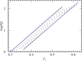
Figure 8: Fitting relation for $Q(X,Z=Z_{\odot},\Gamma_{\rm e})$. Black crosses indicate numerically determined values of $Q$, for $X=0$ – 0.7. Blue lines indicate our fitting relation Eq. 28, for $X=0$ (top), and $X=0.7$ (bottom).

The values of $Q$ determined this way, lie between $Q\sim 1$, and $Q\sim 150$ (cf. Fig. 8), with $\Gamma_{\rm e}=0.3$–0.6. For lower $Q$ (i.e., lower $\Gamma_{\rm e}$), the extension of the Fe-peak becomes so small that it does not cover a factor $f_{P}=10$ in $P_{\rm gas}$. Under these conditions an envelope inflation may still occur, however only of moderate strength. For $Q$ larger than $\sim 150$, $\rho_{\rm min}$ becomes so small that the range of the opacity tables is exceeded. In this case we still expect a very strong envelope inflation, but are just not able to infer $Q$ from the tables.

For given $Q$, $W$ can be determined from Eq. 26. If we additionally allow for clumping with a clumping factor $D$ (cf. Sect. 2.4), we have $\bar{\rho}=(f_{\rho}/D)\rho_{\rm min}$, i.e., we can express $W$ in the form

$$W=\frac{R\,\Delta P}{GM\rho_{\rm min}(f_{\rho}/D)}=\frac{Q(X,Z,\Gamma_{\rm e})}{(f_{\rho}/D)}\frac{(R/R_{\odot})}{(M/M_{\odot})},$$ (29)

with $f_{\rho}\approx 2$.

To compute the envelope extension $\Delta R$ for a star with given parameters $M$, $L$, $X$, and $R$ (where $R$ may denote $R_{\rm c}$ or $R_{\rm e}$), the following steps thus need to be performed.

• For given $M$, $L$, and $X$, $\Gamma_{\rm e}$ can be computed from Eq. 6.

• For given $X$, and $\Gamma_{\rm e}$, $Q$ can be estimated from Eq. 28.

• For given $Q$, $W$ can be determined from Eq. 29, adopting reasonable values for $f_{\rho}$, and $D$. Note that the stability limit Eq. 24 can be expressed in the form $Q/(f_{\rho}/D)<M/R$ (in solar units).

• Finally, for given $W$, the radial extension $\Delta R$ can be computed from Eq. 22, or Eq. 23.

E.g., for our He models in Table 1 (with $X=0$), masses are typically of the order of $15\,M_{\odot}$, and core radii are $\sim 1\,R_{\rm sun}$, i.e., $M/R\sim 15$ in solar units. This means that an unstable situation, with $W=1$, is reached for $Q/(f_{\rho}/D)\sim 15$ (cf. Eq. 29). For $f_{\rho}=2$, and $D=1$, this corresponds to $Q\sim 30$. According to Eq. 28 this value is reached for $\Gamma_{\rm e}\sim 0.4$, in agreement with our models with $D=1$ in Table 2. For a large clumping factor $D=16$, a value of $W=1$ is already reached for $Q\sim 2$, suggesting an instability at $\Gamma_{\rm e}\sim 0.3$, in agreement with our models with $D=16$ in Table 2.

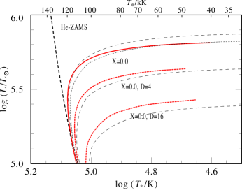
Figure 9: HR diagram for pure He models (red), compared with our analytical relations. Long-dashed lines: analytical relation with $f_{\rho}=2$, short-dashed line: analytical relation with $f_{\rho}=1.5$.

In Fig. 9 we compare our analytical predictions, based on core radii $R_{\rm c}$ from Langer (1989b), with our numerical models. Long-dashed lines indicate predicted HRD positions within our analytical formalism for clumping factors $D=1$, 4, and 16, and an adopted $f_{\rho}=2$. The short-dashed line indicates the results for $f_{\rho}=1.5$, and $D=1$. Note that the use of the He-ZAMS models by Langer introduces inconsistencies. Nevertheless, our formalism describes the envelope inflation very well, in particular its dependence on the clumping factor $D$. Also the uncertainty due to the adopted $f_{\rho}$ turns out to have only moderate influence on the results.

3.4 The mass of the surrounding shell $\Delta M$

The mass $\Delta M$ of the dense shell surrounding the inflated zone (cf. Fig. 1) may be of interest, e.g. in relation to the energy budget, and the timescales of variations in $\Delta R$.

To compute $\Delta M$ we use the following assumptions. 1) The radial extension of the shell is small compared to the total stellar radius, i.e., $r=R_{\rm e}$. 2) The mass of the shell is small compared to the stellar mass, i.e., $m=M$. 3) The pressure $P$ at the stellar surface is small compared to the pressure at the outer boundary of the inflated region $P_{\rm e}$.

Under these assumptions, the equation of hydrostatic equilibrium (Eq. 1) can be integrated directly, and we obtain

$$\Delta M=P_{\rm e}\frac{4\pi R_{\rm e}^{4}}{GM}.$$ (30)

The mass of the shell thus simply follows from the fact that the pressure force $P_{\rm e}4\pi R_{\rm e}^{2}$ at the rim of the low density region needs to be in equilibrium with the gravitational force $GM\Delta M/R_{\rm e}^{2}$ on the shell. Again, $P_{\rm e}$ depends on material properties. Using $P_{\rm e}\approx 0.4...0.9$$\cdot$$10^{6}\,{\rm dyn}/{\rm cm}^{2}$ from our models (cf. Table 1 and 2), we obtain

$$\Delta M/M_{\odot}\approx 0.5...1.0$$\cdot$$10^{-9}\,\frac{(R_{\rm e}/R_{\odot})^{4}}{M/M_{\odot}}.$$ (31)

$\Delta M$ thus mainly depends on the radius of the star. This is in agreement with our model computations (Table 1 and 2) where we find $\Delta M$ as low as $10^{-9}\,M_{\odot}$ for compact WR stars, whereas our larger, LBV-type models reach $\Delta M$ up to $10^{-2}\,M_{\odot}$.

3.5 Dependence on model assumptions

The occurrence of an envelope inflation, involving a density inversion, has been reported in many previous works. Examples are the Wolf-Rayet models by Schaerer (1996), and models for very massive main sequence stars, as well as hydrogen-deficient carbon stars, by Saio et al. (1998). What all these stars have in common, is their proximity to the Eddington limit. Especially the latter work, which discusses the connection of inflated envelopes to the strange-mode instability, demonstrates the universality of the principles discussed here, for stars covering the range of 0.9–110 $M_{\odot}$.

On the other hand, the inflation effect has not been detected in many standard works on stellar evolution. E.g., in the rotating evolutionary models by Meynet & Maeder (2003), the $120\,M_{\odot}$ track enters the H-free WR stage with a mass of $23.2\,M_{\odot}$, and an effective core temperature of $T_{\star}=123$ kK. According to our results in Table 1, we would expect a considerable envelope inflation, with $T_{\star}\sim 60\,$kK, for the same object. In this section we discuss possible sources of such discrepancies, such as the influence of the imposed outer boundary condition (Sect. 3.5.1), dynamical terms on a secular timescale (Sect. 3.5.2), dynamical terms introduced by mass-loss (Sect. 3.5.3), and the treatment of convection and turbulence (Sect. 3.5.4).

3.5.1 The effect of the outer boundary condition

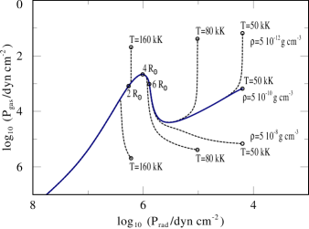
Figure 10: The effect of $\rho$ and $T$ at the outer boundary, on the envelope solution. The solid blue line indicates our standard $23\,M_{\odot}$ He-model in the $P_{\rm rad}$–$P_{\rm gas}$ plane. The dashed lines indicate solutions for which the boundary values for the density $\rho$, and the temperature $T$ have been changed. The inflated zone between 2 and 6 $R_{\odot}$ (as indicated by the radius marks) is mainly affected by the choice of the temperature $T$ at the outer boundary. Temperatures $T\gtrsim 80$ kK, can lead to a cut-off of the inflated zone.

In Fig. 10 we illustrate the influence of the adopted boundary values for $\rho$, and $T$, on the envelope solution. The blue line indicates our standard $23\,M_{\odot}$ He-model, with boundary values $T=50$ kK, and $\rho=5$$\cdot$$10^{-10}{\rm g}\,{\rm cm}^{-2}$. In addition we show six test models (dashed lines), for which we have changed $\rho$ to values of $5$$\cdot$$10^{-8}{\rm g}\,{\rm cm}^{-2}$ and $5$$\cdot$$10^{-12}{\rm g}\,{\rm cm}^{-2}$, for temperatures of $T=50$, 80, and 160 kK.

Firstly, the envelope solution turns out to be very robust with respect to changes of the outer boundary. For increasing $P_{\rm rad}$, i.e., towards the interior of the star, all test models merge into the standard solution. However, boundary temperatures in the region of the Fe-opacity peak, i.e., temperatures that would lie within the inflated zone, lead to a cut-off of the inflated envelope. In Fig. 10, the inflated zone is indicated by radius marks (2–$6\,R_{\odot}$). Models with outer boundary temperatures $T\gtrsim 80$ kK display envelopes where the inflated zone ends close to the respective outer boundary temperature, i.e. the radii are significantly reduced.

Boundary conditions that take the back-warming effect of an optically thick wind into account, as the ones discussed by Schaerer (1996), may thus inhibit an envelope inflation (Schaerer indeed detected a very similar effect in his model computations). In the same way, strong stellar winds with high temperatures at the wind base, as the ones described by Gräfener & Hamann (2005) for early WC subtypes, will prevent the formation of inflated envelopes. This is not surprising, as such winds are initiated by the hot Fe-opacity peak, i.e., the Fe-opacity peak lies within the wind. We thus expect a strong influence of the detailed wind physics on the inflation effect.

3.5.2 Dynamical terms on a secular timescale

The contraction/expansion of a star during its evolution can lead to energy sources/sinks, in addition to the nuclear energy production rate $\epsilon$, which is included in our models (Eq. 3). To estimate the importance of this effect, we compare the gravitational energy $E_{\rm g}$, which is gained, or lost on a timescale $\tau$, with the stellar luminosity $L$, and estimate in this way a limiting timescale

$$\tau=\frac{\Delta E_{\rm g}}{L}=\frac{\Delta M(M-\Delta M)G}{LR}.$$ (32)

Here $\Delta M$ is the mass of the layers involved in the contraction/expansion, and $R$ is a typical radius.

Because Wolf-Rayet stars are very compact, and evolve on relatively short timescales, such gravitational terms may play a role in their evolution. However, as the masses of the inflated envelopes discussed here are very small, these terms play no role for the inflation effect. For our 23.7 $M_{\odot}$ He-model, which represents the most extreme case of an inflated envelope, we estimate $\tau=0.5$ d, based on the parameters from Table 1, and $R=R_{\rm c}$. We thus expect no influence of secular changes on the inflation effect. In Sect. 4.2 we will discuss the case of LBVs, for which gravitational terms indeed seem to play a role on timescales of the observed S Dor-type variability.

For the complete radiative envelope of a typical WR star (here we use the $15\,M_{\odot}$ model from Table 1, with $\Delta M=1.5\,M_{\odot}$, and $R=0.4\,R_{\odot}$) we estimate $\tau=5000$ yr. Particularly in the end phases of the WR evolution, gravitational terms may thus play an important role in determining the $L/M$ ratio of WR stars, which is an important input for our formalism.

3.5.3 Dynamical terms due to mass-loss

Because of the low densities, mass loss may introduce considerable velocity fields within the inflated envelopes, via the equation of continuity $\dot{M}=4\pi\rho\varv r^{2}$. The effect of the resulting dynamical terms on the envelope structure has been investigated by Petrovic et al. (2006). They found that strong mass loss can inhibit the formation of inflated envelopes, if the velocities within the inflated zone exceed the local escape speed, i.e., when $\varv({\rm d}\varv/{\rm d}r)\approx\varv^{2}/r$ has the same order of magnitude as $GM/r^{2}$. This condition imposes an upper limit for the mass-loss rate

$$\dot{M}_{\rm 0}=4\,\pi\rho_{\rm min}R_{\rm m}^{2}\sqrt{\frac{MG}{R_{\rm m}}},$$ (33)

where we have taken into account that the maximum velocity is reached close to $R_{\rm m}=(R_{\rm e}+R_{\rm c})/2$, where $\rho\approx\rho_{\rm min}$. An inspection of the dynamical term that would result from the density structure within our own models, suggests however that this limit should be lowered by $\sim$ 0.4 dex.

In Table 3 we have compiled conservative estimates of $\dot{M}_{\rm 0}$, based on $\rho_{\rm min}=5$$\cdot$$10^{-11}\,{\rm g}/{\rm cm}^{3}$, for a set of WR, and LBV models. For the WR models with the lowest temperatures, which may be subject to an envelope inflation, we find $\log(\dot{M}_{\rm 0}/M_{\odot}{\rm yr}^{-1})=-4.2$…$-3.7$. For comparison, spectroscopically determined mass-loss rates by Hamann et al. (2006) reach values of up to $\log(\dot{M}/M_{\odot}{\rm yr}^{-1})=-4.3$…$-4.1$, dependent on $L$. In view of the involved uncertainties, it is thus not clear whether the envelope inflation of WR stars is affected by dynamical effects.

Table 3: Estimated limiting mass-loss rates $\dot{M}_{\rm 0}$ according to Eq. 33, based on an adopted value of $\rho_{\rm min}=5$$\cdot$$10^{-11}\,{\rm g}/{\rm cm}^{3}$.

$\log(L)$	$X$	$T_{\star}$	$M$	$R_{\rm c}$	$R_{\star}$	$R_{\rm m}$	$\log(\dot{M}_{\rm 0})$
$[L_{\odot}]$		$[{\rm kK}]$	$[M_{\odot}$]	$[R_{\odot}]$	$[R_{\odot}]$	$[R_{\odot}]$	$[M_{\odot}/{\rm yr}]$
5.8	0.0	100	24	1.7	2.6	2.2	-4.3
5.8	0.0	75	24	1.7	4.7	3.2	-4.1
5.8	0.0	50	24	1.7	10.6	6.2	-3.7
5.3	0.0	100	12	1.0	1.5	1.3	-4.8
5.3	0.0	75	12	1.0	2.6	1.8	-4.6
5.3	0.0	50	12	1.0	6.0	3.5	-4.2
6.15	0.36	17	73	14	137	59	-1.9
6.12	0.36	28	70	14	51	30	-2.4

3.5.4 Convection and turbulence

As already noted in Sects. 2.2, and 3.1, the inefficiency of convection is a mandatory condition for the occurrence of an envelope inflation. As the convective efficiency may be affected by details of the numerical implementation, or effects that are not taken into account in the standard mixing-length approach, we give basic physical arguments, why the convective efficiency should be low for the cases discussed in this work.

Generally, the strong increase in opacity near the iron bump will lead to the onset of convection through the usual Schwarzschild stability criterion. But for the models here such convection should be quite inefficient in the sense that it can carry only a small fraction of the local stellar flux $F$. To see this, note that a robust upper limit to the flux carried by convection is set by the free-streaming of internal energy $U$ at the local sound speed $\varv_{\rm s}$, $F_{\rm fs}=\varv_{\rm s}U$. In general, $U=U_{\rm gas}+U_{\rm rad}$, but in the luminous stars here, and particularly in the region around the iron bump, the radiative energy dominates. The associated maximum fraction of stellar flux $F$ that could be carried by convection is thus

$$\frac{F_{\rm fs}}{F}\approx\varv_{\rm s}\frac{U_{\rm rad}}{F}=\frac{4\varv_{\rm s}}{c}\,\left(\frac{T}{T_{\rm c}}\right)^{4}\approx 0.0034\left(\frac{10^{5}\,{\rm K}}{T_{\rm c}}\right)^{4}\,,$$ (34)

where $T_{\rm c}$ is the effective temperature for the (pre-inflated) core radius $R_{\rm c}$. The last equality applies the characteristic iron bump temperature $T\approx 1.5\times 10^{5}$ K, with associated sound speed $\varv_{\rm s}\approx 50$ km/s. This shows directly that for core effective temperatures appropriate for Wolf-Rayet stars, convection can carry only a small fraction of the total stellar flux, viz. 0.3% for $T_{\rm c}=10^{5}$ K, and about 5% for $T_{\rm c}=50,000$ K. This implies that, even when convection sets in, the bulk of the stellar flux is still transported by radiative diffusion, thus justifying this basic simplifying assumption in our analysis of envelope inflation.

We note that, due to the dominance of radiation pressure, and radiation energy in the inflated zone, the contributions from internal gas pressure/energy are generally negligible with respect to $F_{\rm fs}$. The same holds for turbulent pressure/energy, as $P_{\rm turb}=(2/3)u_{\rm turb}=(1/3)\rho a^{2}{\cal M}^{2}$ is of the same order of magnitude as gas pressure/energy (cf., Maeder 2009, p. 105). Here $u_{\rm turb}$ denotes the turbulent energy density, $a$ the sonic speed, and ${\cal M}$ the Mach number, which is expected to be lower than one.

For low convective efficiency, the structure of inflated envelopes is solely determined by Eq. 16, which is (in first order approximation) equivalent to the condition that $\Gamma=1$. The latter only follows from material properties, so that the addition of turbulent pressure has almost no effect on the resulting envelope structure.

4 Implications

Let us next discuss the implications of the predicted envelope inflation for stars close to the Eddington limit, i.e., for WR stars and LBVs. Both types of objects are extremely luminous, and are thought to reside close to the Eddington limit. In Sect. 4.1, we focus on the still unexplained WR locations in the HR diagram. In Sect. 4.2, we discuss the possible connection of the radius inflation to the S Doradus radius changes characteristic of LBVs.

4.1 The radius problem for Wolf-Rayet stars

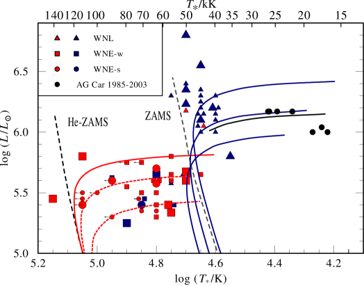
Figure 11: Herzsprung-Russel diagram of the Galactic WN stars, and the LBV AG Car. Red/blue symbols indicate observed HRD positions of WN stars from Hamann et al. (2006) (blue: with hydrogen ($X>0.05$); red: hydrogen-free ($X<0.05$)). Black symbols indicate the HRD positions of AG Car throughout its S Dor Cycle from 1985–2003, according to Groh et al. (2009b). Large symbols refer to stars with known distances from cluster/association membership. The symbol shapes indicate the spectral subtype (see inlet). Arrows indicate lower limits of $T_{\star}$ for stars with strong mass loss. The observations are compared to stellar structure models with/without hydrogen from this work (blue/red lines, cf. Fig. 6), and for AG Car ($X=0.36$, black line).

In Fig. 11, we show an HR diagram for galactic WR stars, as obtained from spectral analyses by Hamann et al. (2006). As already highlighted by these authors there exists a radius problem for H-free WR stars, namely that these objects are not located on the theoretical He-main sequence. According to a population synthesis performed by Hamann et al., almost all WR stars with a hydrogen surface abundance $X<0.05$ are expected to display stellar temperatures $T_{\star}$ in excess of 100 kK. However, in the observed HR diagram they cover a broad temperature range from 40–140 kK, with the majority below 100 kK (red symbols in Fig. 11). The observed WR radii are thus larger than predicted by stellar structure models (e.g., Langer 1989b).

At this point we note that the stellar temperatures $T_{\star}$, as determined by Hamann et al. (2006), are not classical effective temperatures (related to $\tau=2/3$), but effective temperatures, related to the (hydrostatic) surface radius $R_{\star}$, i.e.,

$$T_{\star}=\left(\frac{L}{4\pi\,\sigma_{\rm SB}\,R_{\star}^{2}}\right)^{\frac{1}{4}},$$ (35)

with the Stefan-Boltzmann constant $\sigma_{\rm SB}$. $R_{\star}$ is the inner boundary radius of the employed atmosphere models, and is typically located at a much higher optical depth of $\tau_{\rm max}\approx 20$. As long as $R_{\star}$ is located in the hydrostatic part of the wind, its value does not depend on the detailed choice of $\tau_{\rm max}$ . The $T_{\star}$ determined by Hamann et al. thus reflect actual surface radii, which are not affected by the optical depth of the strong stellar winds of WR stars. The low $T_{\star}$ in Fig. 11 thus display a true inconsistency with respect to the stellar structure models.

This is particularly surprising, as H-free WR stars are very simple objects. Due to their large convective cores, and high mass-loss rates they are expected to be close to chemical homogeneity (Langer 1989a). Even if the material in their He-burning cores is partly processed to carbon and oxygen, the mean molecular weight stays almost constant throughout the star. Moreover, the strong temperature sensitivity of He-burning guarantees an almost fixed temperature in their centers. The main unknown for the determination of the stellar structure is thus the opacity. In fact, with the advent of the OPAL opacity data (Iglesias & Rogers 1996) and their strong Fe-opacity peaks, Ishii et al. (1999) were the first to predict the large envelope inflation that we also describe in this work.

Ishii et al. (1999) could however not explain the HRD positions of these stars. In the galaxy, most H-free WR stars are located at luminosities below $\log(L/L_{\odot})\approx 5.8$, reaching down to $\log(L/L_{\odot})\approx 5.3$ (cf. Fig. 11). Ishii et al. demonstrated that unrealistically high metallicities, up to $Z=0.1$, would be needed to achieve a significant radius inflation in this regime. An important result of the present work is that the same effect can be achieved by the assumption of an inhomogeneous (clumped) structure within the inflated zone (cf. Sect.2.4). For moderate clumping factors, up to $D=16$, our models cover the observed parameter range (red (dashed) lines in Figs. 6 and 11). Notably, similar clumping factors are determined spectroscopically, for the winds of WR stars (e.g., Hamann & Koesterke 1998).

The metallicity dependence, as predicted by Ishii et al. (1999) and Petrovic et al. (2006), may however still play an important role in the determination of the temperatures of WR stars, as their subtype distribution seems to depend on $Z$ (e.g., Crowther 2007). Later spectral subtypes are typically found at higher $Z$, which is in line with a stronger radius inflation due to the stronger Fe-opacity peak at higher $Z$. This effect may however also depend on the increased mass loss at higher $Z$ (see Crowther & Hadfield 2006). We further note that, as discussed in Sect. 3.5.3, the mass-loss limit by Petrovic et al. (2006) may inhibit an envelope inflation for WR stars with strong mass-loss.

4.2 Radius changes of S Doradus-type LBVs

A defining property of LBVs are S Doradus-type radius variations on timescales of months to years. The inflation effect provides a reasonable explanation for radius variations on such timescales, as only small portions of the stellar envelope are affected. The underlying reason for the time dependence may be manifold. E.g., Georgiev et al. (2011) recently proposed that the variability of HD 5980, an LBV-like star that temporarily shows a WR-type spectrum, may be triggered by a transition from a hot, to a cool wind base. This picture fits very nicely into the framework of the inflation effect. As discussed in Sect. 3.5.1, we expect that a hot, optically thick wind would inhibit a radial inflation, i.e., a wind transition as proposed by Georgiev et al. could indeed lead to substantial radius changes.

In the following we discuss the case of AG Car, one of the best-studied galactic S Doradus LBVs (e.g., Leitherer et al. 1994; Stahl et al. 2001; Vink & de Koter 2002). More recently, AG Car has been studied in detail throughout its full S Dor cycle (1985–2003), by Groh et al. (2009b, 2011). During this period the star increased its radius from $58.5\,R_{\odot}$ to $120.4\,R_{\odot}$, corresponding to a change in the stellar temperature from $T_{\star}=26,450$ K to 16,650 K. Such radius and temperature changes are characteristic aspects of the S Dor cycle, but they remain as yet unexplained by stellar structure calculations (see however Stothers & Chin 1993). For AG Car the luminosity was found to decrease from $\log(L/L_{\odot})=6.17$ to 6.0 between the S Dor visual minimum and maximum phase. Furthermore, Groh et al. (2009b) determined a considerable hydrogen deficiency for AG Car, with a hydrogen surface mass fraction of $X=0.36$.

We have computed a series of homogeneous stellar structure models for the relevant parameter range, with a hydrogen mass fraction of $X=0.36$, and masses ranging from 60–$73\,M_{\odot}$ (cf. Table 2). These models display a similar luminosity range as AG Car, and partly show very low $T_{\star}$, down to $\sim$ 17,000 K, due to a substantial radius inflation. A comparison with the observed HRD positions of AG Car is shown in Fig. 11. Notably, during the minimum phases of the S Dor cycle, AG Car (indicated by black symbols) shows a very good agreement with our homogeneous models (black dashed line), i.e., its position in the HR diagram can be explained by a chemically homogeneous star with $M\sim 70\,M_{\odot}$, and a substantial radius inflation.

The core of such a star would be relatively small, with $R_{\rm c}\sim 14\,R_{\odot}$, corresponding to an effective core temperature $T_{\rm c}\sim 53$ kK (cf. Table 2). Due to the envelope inflation, the star would display a core-halo structure, as described in Sect. 2.2. According to Eq. 31, the mass $\Delta M$, of the outer shell around the inflated envelope, is expected to change throughout the S Dor cycle. For the smallest radius ($58.5\,R_{\odot}$), we obtain $\Delta M\sim 10^{-4}M_{\odot}$, while $\Delta M\sim 2$$\cdot$$10^{-3}M_{\odot}$ for the largest extension ($120.4\,R_{\odot}$). The energy to lift this material from the core radius to the stellar surface is $\Delta E_{\rm g}\sim\Delta MMG/{R_{\rm c}}=3.8$$\cdot$$10^{46}\,{\rm erg}$. This value compares well with the ’missing energy’ due to the decrease in luminosity $\Delta E_{\rm lum}=1.83$$\cdot$$10^{39}{\rm erg/s}\times 575{\rm d}=9.1$$\cdot$$10^{46}{\rm erg}$ (cf.  Groh et al. 2009b). We thus find that within the inflated envelope, the S Dor-type variability introduces dynamical effects as the ones discussed in Sect. 3.5.2.

The good agreement with our models suggests that the extension of the envelope of AG Car may be explained by the inflation effect. The mass-loss rate of AG Car ($\log(\dot{M}/M_{\odot}{\rm yr}^{-1})<-4.2$, Groh et al. 2009b) lies well below the upper mass-loss limit discussed in Sect.3.5.3 (cf. Table 3), implying a stable, static configuration that is not affected by dynamical effects due to mass loss. Based on our chemically homogeneous models, AG Car lies close to the Eddington limit, with an Eddington factor of $\Gamma_{\rm e}=0.39$. According to Eq. 28, this results in a $Q$ parameter of $\sim 9$, and with Eq. 29 we obtain $W_{\rm c}\sim(9/f_{\rho})(R_{\rm c}/R_{\odot})/(M/M_{\odot})\sim 0.8$ (where we have adopted $f_{\rho}=2.2$ from Table 2). The star is thus very close to the instability limit ($W_{\rm c}=1$), as discussed in Sect. 3.2.

One possible mechanism that could lead to an unstable situation involving $W_{\rm c}>1$, is the reduction of the effective stellar mass through rotation. Groh et al. (2011) found that the observed rotational velocity of AG Car declines from $\varv_{\rm rot}\sin i=220\,$km/s in the minimum phase, to 90 km/s for the largest extension. For these values the ratio of centrifugal to gravitational acceleration at the stellar surface decreases from $\varv_{\rm rot}^{2}R_{\star}/(GM)=0.21/\sin^{2}i$, to $0.07/\sin^{2}i$. The corresponding reduction of the effective stellar mass by 20% in the minimum phase, could thus just lead to a situation where $W_{\rm c}\approx 1$. In this case the outer stellar envelope would become unstable, and could start expanding. The reduction of the rotational velocity during the expansion would lead to $W_{\rm c}<1$, and a re-stabilization of the envelope.

Groh et al. (2009a, 2011) proposed a somewhat similar scenario for AG Car, where the Eddington limit is exceeded due to rotation. In this work, we have demonstrated that already for moderate Eddington factors of $\Gamma_{\rm e}\sim 0.4$ AG Car may form an inflated stellar envelope that is dominated by radiation. Within this envelope the star adjusts very precisely to the Eddington limit ($\Gamma=1$). In our scenario, the instability that potentially induces the S Dor cycle is due to the fact that the specific internal energy due to radiation exceeds the gravitational potential, with the stellar envelope thus becoming unbound.

We want to point out that the formation of inflated envelopes does not depend on the assumption of chemical homogeneity in our numerical models. The instability follows from our formalism in Sect. 3, and is thus independent of the internal structure of the star. For AG Car, the observed luminosity ($\log(L/L_{\odot})=6.17$), and surface hydrogen mass fraction ($X=0.36$) imply a mass of $74\,M_{\odot}$ for the case of chemical homogeneity (cf. Gräfener et al. 2011). In reality, AG Car is likely more chemically enriched in the core, i.e., its mass is lower, and its core radius larger. This would lead to an even earlier onset of the inflation effect, and its instability. As the evolutionary status of LBVs is not well known, it is however not possible to obtain reliable mass estimates for this type of object.

5 Conclusions

In the present work, we have discussed the possible formation of radially inflated stellar envelopes for stars approaching the Eddington limit, as originally proposed by Ishii et al. (1999), and Petrovic et al. (2006). In addition to numerical models, we could provide an analytic description of this process, leading to the discovery of a new instability limit, and a clumping dependence. Both effects turn out to be of profound importance. While the former may be connected to S Doradus-type instabilities in LBVs, the latter can account for the large observed radii of Galactic WR stars, and thus resolve the long standing WR radius problem.

Within our analytical approach we could describe the inflation effect in terms of a dimensionless parameter $W$ (Eqs. 28, 29) that characterizes the ratio between internal and gravitational energy at the base of the envelope. $W$ can be estimated on the basis of opacity tables and a combination of stellar parameters. The envelope inflation occurs when $W$ approaches one. For $W\geq 1$, we find that the envelope becomes gravitationally unbound, i.e., there exists no static solution. A prerequisite for envelope inflation is the proximity of the star to the Eddington limit, with Eddington factors of $\Gamma_{\rm e}>0.3$–0.35, at solar metallicity. For a given chemical composition and $\Gamma_{\rm e}$, the resulting stellar radius depends on the ratio $M/R$, and on the degree of (in)homogeneity of the material within the envelope (characterized by a clumping factor $D$).

Envelope inflation has a strong impact on the effective temperatures of stars in the upper HR diagram. For Wolf-Rayet stars it can account for the ’radius problem’, i.e., that the observed stellar temperatures of H-free WR stars are much lower than predicted by canonical stellar structure models. To reproduce the observed HRD positions of these objects, it is necessary to assume that the material within the envelope is clumped. The resulting clumping factors lie in the range of $D=1$–16, in notable agreement with typical clumping factors detected in the winds of WR stars (e.g., Hamann & Koesterke 1998). As the envelope inflation is expected to depend on metallicity (Ishii et al. 1999; Petrovic et al. 2006), it may also account for the observed $Z$-dependence of the spectral subtype distribution of WR stars, i.e., that WR stars in high-$Z$ environments show lower effective temperatures (e.g., Crowther 2007).

For the luminous blue variable AG Car we suggest that the observed HRD position of a $\sim$ $70\,M_{\odot}$ star, with a relatively compact core, might be subject to substantial envelope inflation. During its S Dor cycle, AG Car is found to increase its radius by a factor of two, while its luminosity decreases by a factor of 1.5. The luminosity decrease might be explained as a result of the formation of a dense outer shell with a mass of $\sim 2$$\cdot$$10^{-3}\,M_{\odot}$ as predicted by our models. The energy needed to lift this material from the core to the outer radius is of the same order of magnitude as the ’missing energy’ due to the decrease in luminosity. Similar to the mechanism proposed by Groh et al. (2009a, 2011), the S Dor variability of AG Car may be due to the effect of stellar rotation, which reduces the effective stellar mass, and thus leads to an instability with $W>1$, that forces the star to expand.

We conclude that the stellar effective temperatures in the upper HR diagram are potentially strongly affected by the inflation effect. The peculiar structure of the inflated envelopes, with an almost void, radiatively dominated region, beneath a thin and dense shell could mean that many, rather very compact stars, are hidden below inflated envelopes, and thus display much lower effective temperatures to the observer. Also compact, fast rotating stars may be hidden this way. This may particularly affect massive stars just before the final collapse, and the question of whether they form a SN Ibc, or a GRB (for the latter smaller core radii are inferred than the observed WR radii, cf. Cui et al. 2010). The complex envelope structure may also affect the early X-ray afterglow of GRBs (e.g. Li 2007).