Identifying Star Streams in the Milky Way Halo

Abstract

We develop statistical methods for identifying star streams in the halo of the Milky Way galaxy that exploit observed spatial and radial velocity distributions. Within a great circle, departures of the observed spatial distribution from random provide a measure of the likelihood of a potential star stream. Comparisons between the radial velocity distribution within a great circle and the radial velocity distribution of the entire sample also measure the statistical significance of potential streams. The radial velocities enable construction of a more powerful joint statistical test for identifying star streams in the Milky Way halo. Applying our method to halo stars in the Hypervelocity Star (HVS) survey, we detect the Sagittarius stream at high significance. Great circle counts and comparisons with theoretical models suggest that the Sagittarius stream comprises 10% to 17% of the halo stars in the HVS sample. The population of blue stragglers and blue horizontal branch stars varies along the stream and is a potential probe of the distribution of stellar populations in the Sagittarius dwarf galaxy prior to disruption.

1. INTRODUCTION

The timescale for halo stars to exchange their energy and angular momentum is long compared to the age of the Milky Way galaxy. Thus, the stellar halo of the Milky Way provides a unique laboratory for studying hierarchical galaxy formation. Theoretical simulations show that the remnant debris of hierarchical galaxy formation should be visible as star streams in the Milky Way halo (Johnston et al., 1996; Harding et al., 2001; Abadi et al., 2003; Bullock & Johnston, 2005; Font et al., 2006). Indeed, observers have discovered the tidal debris of the Sagittarius dwarf galaxy (Ibata et al., 1994) wrapping around the Milky Way (Majewski et al., 2003) and other stellar overdensities throughout the stellar halo (e.g., Belokurov et al., 2006). The vast majority of these detections come from star counts without radial velocity measurements.

We describe a powerful technique for identifying tidal star streams that exploits the additional information provided by a complete radial velocity survey. With large stellar radial velocity surveys such as RAVE (Steinmetz et al., 2006; Zwitter et al., 2008) and SEGUE (Yanny et al., 2009) now available, approaches including radial velocities enable better constraints on structure in the halo.

To identify statistically significant tidal structures, we examine the surface number distribution and the radial velocity distribution of stars in great circles. Both the surface density and the radial velocity distributions probe the origin of structure in the halo. A radial velocity test for structure applies independently of the underlying spatial distribution. Our technique opens up the possibility of finding tidal star streams based on structure in velocity space. Combining our spatial and radial velocity statistical tests provides a more powerful joint test for identifying star streams.

Previous studies of positions and velocities have focused on known tidal streams, such as Sagittarius (e.g., Yanny et al., 2009; Ruhland et al., 2011), or have analyzed disconnected patches scattered across the sky (Starkenburg et al., 2009; Schlaufman et al., 2009). Known tidal debris, however, is contiguous over areas of hundreds or thousands of square degrees (Johnston et al., 1999; Ibata et al., 2001).

As a first demonstration of our technique, we search for structure in the HVS radial velocity survey, a complete, non-kinematically selected sample of late B-type stars covering a contiguous area of more than 8400 deg² on the sky (Brown et al., 2005, 2006b, 2009a, 2010). The HVS survey targets blue stragglers and blue horizontal branch (BHB) stars within the halo and is distinct in its uniform velocity data for a well-defined sample of potential halo stars.

We detect significant structure in the sample of halo stars within the HVS survey. Most of this structure is attributed to the Sagittarius stream. We compare our detections with the Law & Majewski (2010) N-body model for the Sagittarius dwarf, derive estimates for the fraction of HVS stars within the Sagittarius stream, and assess the relative fractions of blue stragglers and BHB stars along the stream.

In §2, we describe the statistical technique. In §3, we apply this technique to the HVS survey. In §4, we compare the survey stars with the $N$-body model of Law & Majewski (2010) in order to explore the nature and surface density of stars within the Sagittarius stream. We conclude in §5.

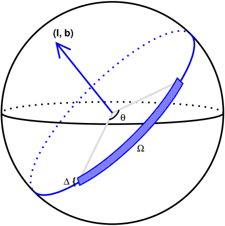
Figure 1.— Solid angle, $\Omega$, subtended by a great circle segment with arc length $\theta$, width $\Delta$, and pole at galactic coordinates $(l,b)$.

2. TECHNIQUE FOR IDENTIFYING STAR STREAMS

Identifying structures in the Galactic halo is a challenging statistical problem. The structures are low contrast and may extend across the entire sky. For most stars in the Galactic halo, we have ready access to only half of phase space. Radial velocity and angular position are the only robust coordinates available for large samples of stars more distant than $\sim 10$ kpc (e.g., Schlaufman et al., 2009).

Methods of identifying star streams and other substructures in the Milky Way halo include pole counts (Lynden-Bell & Lynden-Bell, 1995), great circle counts (Johnston et al., 1996), star count maps (e.g., Ibata et al., 2002; Belokurov et al., 2006), group finding algorithms (Sharma et al., 2011; Xue et al., 2011), and combined analyses of the spatial and radial velocity distributions of halo populations (e.g., Schlaufman et al., 2009). Most of these methods include an assessment of the statistical significance of the structures they detect.

The method we develop contains elements of previous approaches refined for application to radial velocity samples that are complete over some substantial portion of the sky. Our approach has three steps: (1) we analyze great circle counts based on a nearly uniform, dense grid of sampling poles, (2) we compare the great circle radial velocity distribution with the radial velocity distribution for the entire survey, and (3) we combine the great circle counts and velocity distribution comparison into a single statistic. We estimate the significance level, or probability of false positives, among the structures we detect.

2.1. Great Circle Counts

The orbits of tidal debris from disrupted satellite galaxies in the Milky Way halo persist for several Gyr. Because the Galactic halo is approximately spherical, a satellite’s orbit in the sky should approximate a great circle. The “fossil” debris should be distributed along the orbit of the satellite (e.g., Johnston et al., 1996; Bullock & Johnston, 2005).

Johnston et al. (1996) propose using star counts in great circles for detecting tidal debris against background halo stars. They define a great circle by its width and by the position of its pole relative to the Galactic pole. The pole is the unit normal to the plane of the great circle. The latitude and longitude of the pole on the unit sphere then determine the location of its corresponding great circle, as illustrated in Figure 1. Johnston et al. (1996) compare counts of stars observed within a great circle with the number of stars expected from a random distribution of stars on the sky. We generalize this approach for an observational sample that covers only a portion of the sky. For simplicity, we refer to the number of stars in a great circle segment as the great circle count.

For a great circle segment of arc length $\theta$ and width $\Delta$ within the sample region, the solid angle subtended the segment is$\ \Omega=2\theta\sin(\frac{\Delta}{2})\approx\theta\Delta$ for small $\Delta$. The probability, $p$, that a star placed at random in the sample region falls within the great circle segment is the ratio between the area of the segment, $\Omega$, and the area, $\Omega_{sample}$, of the entire sample region (Figure 1)

$$p=\frac{\Omega}{\Omega_{sample}}=\frac{2\theta\sin(\frac{\Delta}{2})}{\Omega_{sample}}\approx\frac{\theta\Delta}{\Omega_{sample}}~{}\text{, for small }\Delta\text{.}$$ (1)

For $n$ stars randomly distributed in the sample region, the number, $k$, of stars in the great circle segment follows a binomial distribution with expected value $E(X)=np$ and variance $Var(X)=np(1-p)$. The cumulative binomial distribution gives the probability, $p_{GC}$, of observing $k$ or more stars in the great circle segment

$$p_{GC}=\Pr(X\geq k)=\sum_{j=k}^{n}\binom{n}{j}p^{j}\left(1-p\right)^{n-j}$$ (2)

We evaluate this expression using the incomplete beta function (Press et al., 1992). This probability measures the statistical significance of each observed great circle count.

We sample the survey region by placing poles on a lattice of Galactic longitude, $l$, and latitude, $b$, derived from a nearly uniform distribution of antipodally symmetric points on the unit sphere using the method of Koay (2011). Note that a pole and its antipode represent the same great circle. We then record observed counts for all segments of great circles corresponding to these poles that lie within the sample boundaries.

To account for multiple statistical tests on the same set of data and to avoid overstating the statistical significance of the findings, we modify the great circle count technique of Johnston et al. (1996). Using the Bonferroni correction (Abdi, 2007), we adjust the probability of each individual test, $p_{GC}$ in equation (2), to account for multiple tests by multiplying the probability by the total number of tests of the data. The Bonferroni correction protects against false positives but at the expense of more false negatives. The Bonferroni correction assumes that the tests are independent and represents a lower bound when they are not. Thus, our estimate of the overall probability of false positives is conservative. In fact, we expect that none of the highest confidence streams we detect in the HVS survey sample are false positives (see §3.2).

2.2. Radial Velocity Distribution

Radial velocities of stars are a potentially important probe for the presence of star streams. The velocity distribution for halo stars is nearly Gaussian with average line-of-sight velocity $v_{rf}=0$ km s^-1 and velocity dispersion $\sigma_{rf}=106$ km s^-1 in the Galactocentric rest frame (Brown et al., 2010). The radial velocity dispersion for stars in a stream should be $\lesssim 10$ km s^-1 (e.g., Harding et al., 2001; Majewski et al., 2004). Relative to the large dispersion of the halo, this small velocity dispersion should enable detection of streams in velocity space.

We search for evidence of streams by comparing the distribution of radial velocities for the stars in a great circle with the observed distribution of radial velocities for the entire sample. If the distribution of radial velocities on the sky is randomly drawn from this underlying distribution, the radial velocities of stars lying in an arbitrary great circle should follow the same distribution. Rather than assuming a Gaussian radial velocity distribution of background halo stars a priori (cf. Harding et al., 2001; Schlaufman et al., 2009), we use the observed radial velocity distribution for the sample. In this approach, the two-sample Kolmogorov-Smirnov test provides a nonparametric estimate of the probability, $p_{V_{rf}}$, that the radial velocity distribution for stars within a great circle is randomly drawn from the same distribution as the HVS survey. We compute $p_{V_{rf}}$ for great circles with poles on the same grid we use for the great circle counts. For each segment of a great circle that lies within the boundaries of the HVS sample, we have $p_{GC}$ and $p_{V_{rf}}$.

We combine the great circle count and radial velocity probabilities to form a joint test under the assumption that spatial position and radial velocity are independent. The probability of observing a group of stars and their radial velocities within a great circle segment of width $\Delta$ is then the product of the individual probabilities for each of these events, $p_{Joint}=p_{GC}\times p_{V_{rf}}$. Although position and radial velocity may not be truly independent, the combined probability gives a measure of the joint departure of the spatial and velocity distributions from those for a set of points randomly distributed on the sphere and randomly drawn from the observed radial velocity distribution.

2.3. Limitations of the Technique

There are several important observational and theoretical limitations to our ability to detect tidal streams. Observational limitations include the limited sky coverage of a sample and the limited depth and density of a sample. Theoretical limitations include departure of the orbit of the stream from a great circle and multiple orbits or wraps of the streams. Harding et al. (2001) review many of the issues involved in detecting tidal debris in the Galactic halo.

Existing radial velocity surveys sample only a fraction of the sky. Consequently, we can only access great circle segments with arc lengths $\theta<360^{\circ}$. The observed magnitude limit of a radial velocity survey defines the volume of the halo and the part of the orbit we sample. We are potentially less sensitive to the apocenter passage than to the pericenter passage of the orbit. More stars are stripped from the progenitor of a star stream near pericenter, probably enhancing our ability to detect streams and possibly leading us to overestimate the density of the stream.

Our sensitivity depends on the width of the great circle that we choose. The overall density of the sample sets a lower limit on the width of great circles we can profitably explore. As we increase the width of the great circles we use to sample the distribution, dilution of potential streams by background stars increases. This problem is particularly serious for the intrinsically narrowest streams.

For computational convenience we approximate orbits as great circles. However, the sun’s offset of approximately 8 kpc from the Galactic center means that orbits do not appear exactly as great circles on the celestial sphere, an effect that diminishes with the size of the orbit and the proximity of the sun to the plane of the orbit. Furthermore, the orbits depart from great circles for a nonspherical Galactic potential.

A nonspherical Galactic potential causes precession of the orbit of the progenitor (Law & Majewski, 2010). Stars stripped during different passes of the progenitor may then appear in the same observed great circle. In our technique, one indication of this phenomenon is the appearance of multiple peaks in the observed radial velocity distribution for the great circle approximating the orbits. Multiple wraps may also increase the great circle count. In addition, intersection with other streams or structures may produce multiple peaks in the radial velocity distribution as well as an increase in the great circle count.

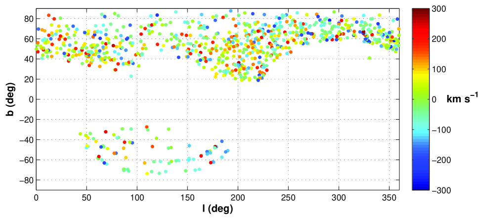
Figure 2.— Galactic coordinates $(l,b)$ of the 881 halo stars in the HVS program survey with $\left|v_{rf}\right|\nolinebreak<\nolinebreak 275$ km s^-1. As indicated in the legend to the right of the main figure, color represents radial velocity in the range $-300$ km s^-1 to $+300$ km s^-1.

3. APPLICATION TO THE HYPERVELOCITY STAR SURVEY

We demonstrate our technique by applying it to the spectroscopic sample of distant halo stars from the HVS survey of Brown et al. (2005, 2006a, 2006b, 2007a, 2007b, 2009a, 2009b). The Brown et al. (2010) catalog of 910 late B-type stars is 93% complete over the magnitude range $17<g_{0}<20.5$ and covers more than $8400$ deg² of the Sloan Digital Sky Survey (SDSS) Data Release 6 (DR6) imaging footprint. These halo stars are a mix of evolved blue stragglers and BHB stars. Because the selection is well understood, this survey and others that cover a large area of the sky uniformly are particularly powerful probes of the halo.

3.1. Data

Brown et al. (2010) measured radial velocities using the Blue Channel Spectrograph on the 6.5m MMT. They derived velocities by constructing appropriate stellar templates and then applying standard cross-correlation routines (Kurtz & Mink 1998). The typical radial velocity uncertainty is $\pm 12$ km s^-1. Brown et al. (2010) transform heliocentric velocities $(v_{helio})$ into Galactocentric rest frame velocities assuming a circular velocity of 220 km s^-1 and a solar motion of $(U,V,W)=(10.0,5.2,7.2)$ km s^-1 (Dehnen & Binney, 1998). For each star, we use this Galactocentric rest frame velocity, $v_{rf}$.

From the 910 stars in HVS survey, we construct a sample of the 881 stars with $\left|v_{rf}\right|<275$ km s^-1. The upper limit on the velocity removes unbound HVSs. The 881 stars in our sample range in heliocentric distance from 12 to 91 kpc. Figure 2 shows the distribution of the sample stars on the sky; the color of the points indicates their radial velocities.

3.2. Great Circle Counts

For the HVS survey, we calculate $p_{GC}$ (equation (2)) for great circles with width $\Delta=5{{}^{\circ}}$. The surface density of stars in the survey constrains $\Delta$. We chose this width by experiment. The survey is too sparse to detect streams with $\Delta<$ 5^∘; adopting $\Delta\geq$ 10^∘ dilutes the signal of streams. Other investigators use $\Delta=5{{}^{\circ}}$ (Majewski et al., 2003), $10{{}^{\circ}}$ (Ibata et al., 2001) and $12{{}^{\circ}}$ (Ibata et al., 2002). We distribute $2.4\times 10^{4}$ antipodally symmetric points nearly uniformly on the unit sphere (Koay, 2011), approximately one pole per $1.7$ square degrees. Since the poles are antipodally symmetric, this represents $1.2\times 10^{4}$ unique great circles. We consider only great circles that intersect the sample region with arc lengths $\theta>25{{}^{\circ}}$. For shorter arcs, small number statistics dominate the results. Our dense grid of sampling poles (§2.1) produces 9884 such great circle segments. Many of these segments overlap.

Figures 3 and 4 show results for the great circle counts derived from the unadjusted $p_{GC}$ without the Bonferroni correction (Figure 3) and the adjusted $p_{GC}$ with the Bonferroni correction (Figure 4). At the position of each pole, we encode $\log_{10}\{1/p_{GC}\}$ in the color scale indicated in the legend. We plot only results with $p$-values of 5% or less ($p_{GC}\leq 0.05$). The plot has an inherent symmetry as poles at antipodes, $(l,b)$ and $(l+180{{}^{\circ}},-b)$, represent the same great circle.

Comparison of these two figures illustrates the effect of accounting for multiple statistical tests applied on the same data set. Applying the Bonferroni correction increases the probabilities that the observed great circle counts result from a random distribution of stars on the sky by a factor of 9884. The values of $p_{GC}^{adjusted}$ in Figure 4 range from $5.0\times 10^{-2}$ to $3.63\times 10^{-9}$.

Using the adjusted $p_{GC}$, the three most significant poles in Figure 4 lie at $(103.1{{}^{\circ}},12.4{{}^{\circ}})$, $(104.5{{}^{\circ}},12.4{{}^{\circ}})$ and $(121.6{{}^{\circ}},20.2{{}^{\circ}})$ with $p_{GC}^{adjusted}=3.63\times 10^{-9}$, $4.99\times 10^{-9}$ and $1.10\times 10^{-8}$, respectively. Features of this significance have much less than a $1\%$ chance of appearing in a random distribution. We list the 25 most significant poles and identify all of them with known structures in Table 1. The two most significant poles coincide with the Sagittarius stream (§3.4 below).

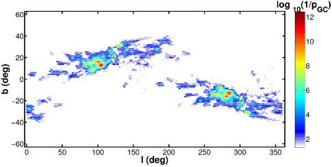
Figure 3.— Significance, $\log_{10}(1/p_{GC})$, of the observed great circle count for pole at $(l,b)$, where $p_{GC}$ represents the unadjusted probability that the observed count results from a random, isotropic distribution of stars, $\theta\geq 25{{}^{\circ}}$ and $\Delta=5{{}^{\circ}}$. As indicated in the legend to the right of the main figure, color denotes significance in the range $\log_{10}(1/p_{GC})$ = 1.5–12.5.

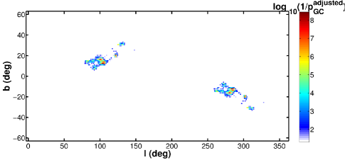
Figure 4.— As in Figure 3 for $\log_{10}(1/p_{GC}^{adjusted})$.

3.3. Using Radial Velocities

Radial velocities provide additional information that aids in identifying star streams, in discriminating among them, and in distinguishing them from other structures. Figure 5 illustrates the power of comparing the velocity distribution for stars in a great circle with the corresponding distribution for the entire HVS survey. The green histogram compares the stellar radial velocity distribution for the great circle with pole at $(89.3{{}^{\circ}},15.0{{}^{\circ}})$ with the velocity distribution for the complete survey (red histogram). For this, the most significant structure in radial velocity in Table 1, the two-sample Kolmogorov-Smirnov test yields a probability of $p_{V_{rf}}=1.47\times 10^{-3}$ that the radial velocities in the great circle were drawn from the same distribution as the entire sample.

The radial velocity distribution within this great circle has two peaks, one at $v_{rf}\approx-80$ km s^-1 and another at $v_{rf}\approx-190$ km s^-1. These peaks do not appear in the distribution for the entire HVS survey sample. The expected radial velocity dispersion within a stream should be $\lesssim 10$ km s^-1; thus, these peaks suggest two distinct physical components in the velocity distribution. In §3.4, we identify this structure in velocity with the Sagitarrius stream.

Using our HVS survey sample, we calculate the probability, $p_{V_{rf}}$, that the radial velocities for stars in the entire sample and for stars within a great circle come from the same distribution for all great circle poles in our grid. Significant poles are located near the significant great circle count pole at $(89{{}^{\circ}},15{{}^{\circ}})$.

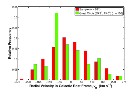
Figure 5.— Distribution of galactocentric radial velocities, $v_{rf}$, for sample stars in the great circle with pole at $(l,b)=(89.3{{}^{\circ}},15.0{{}^{\circ}})$ intersecting Sagittarius stream branch A compared with those of entire sample. The two sample Kolmogorov-Smirnov test yields a probability $p_{V_{rf}}=1.47\times 10^{-3}$ that these two distributions are drawn from the same distribution.

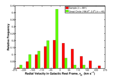
Figure 6.— Distribution of galactocentric radial velocities, $v_{rf}$, for sample stars in the great circle with pole at $(l,b)=(186.6{{}^{\circ}},2.0{{}^{\circ}})$ intersecting the Sagittarius stream and the Virgo overdensity compared with those of entire sample. The two sample Kolmogorov-Smirnov test yields a probability $p_{V_{rf}}=8.31\times 10^{-5}$ that these two distributions are drawn from the same distribution.

The most significant pole based on radial velocity alone has $p_{V_{rf}}=8.31\times 10^{-5}$, appears at $(186.6{{}^{\circ}},2.0{{}^{\circ}})$, and corresponds to a near polar great circle. Figure 6 shows the velocity distribution of the stars in the great circle corresponding to this pole. This detection probably results from two separate substructures, the Sagitarrius stream and the Virgo overdensity (Newberg et al., 2007) as the great circle intersects both. Some stars may belong to the Sagitarrius stream (§4.1). Others may belong to the Virgo overdensity, which has two peaks in its radial velocity distribution at $v_{rf}$ = $-49$ km s^-1 and at $v_{rf}$ = $-171$ km s^-1 (Vivas et al., 2008) that match those of stars in this great circle.

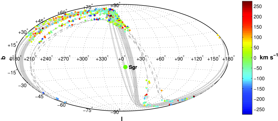
Figure 8.— Great circles in Galactic coordinates $(l,b)$ corresponding to the 25 poles with most significant  $p_{Joint}^{adjusted}=p_{GC}^{adjusted}\times p_{V_{rf}}$. Solid gray lines mark great circles affiliated with the Sagittarius stream. Dashed gray lines denote great circles with superpositions of the Sagittarius stream and other structure. The large green dot labeled Sgr marks the location of the Sagittarius dwarf galaxy. As indicated in the legend to the right of the main figure, color denotes radial velocity in km s^-1.

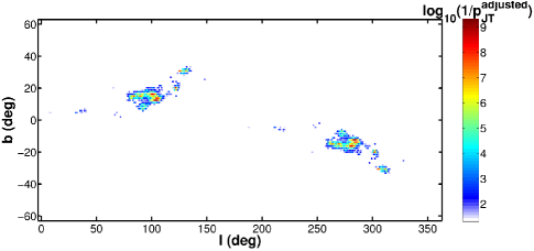
Figure 7.— As in Figure 3 for the adjusted joint probability, $\log(1/p_{Joint}^{adjusted})$, where $p_{Joint}=p_{GC}^{adjusted}\times p_{V_{rf}}$.

Next we combine both spatial and radial velocity information in a joint statistic. Figure 7 shows $p_{Joint}^{adjusted}=p_{GC}^{adjusted}\times p_{V_{rf}}$ at the positions of all of the poles in our grid. We plot $\log_{10}\{1/p_{Joint}^{adjusted}\}$. Many features here are the same as in the map of significant great circle count poles (Figure 4).

We list the 25 most significant poles in $p_{Joint}^{adjusted}$ and their associations with the Sagitarrius stream and other known structure in Table 1. The two most significant poles in Figure 7 and Table 1 correspond to branch A of the Sagittarius stream identified by Belokurov et al. (2006). These poles are also the most significant in $p_{GC}^{adjusted}$ alone and occur at $(103.1{{}^{\circ}},12.4{{}^{\circ}})$ and $(104.5{{}^{\circ}},12.4{{}^{\circ}})$ with $p_{Joint}^{adjusted}=4.63\times 10^{-10}$ and $1.09\times 10^{-9}$, respectively. Although the radial velocity is helpful in selecting other Sagittarius poles, the values for $p_{V_{rf}}$ alone for these two poles are of low significance (Table 1).

3.4. Detection of the Sagittarius Stream

Ibata et al. (2002) analyzed M giant source counts in 26.4% of the sky using the 2MASS Second Incremental Data Release and identified a peak corresponding to a Sagittarius plane with pole at $(95{{}^{\circ}},13{{}^{\circ}})$ for $\Delta$ = $10{{}^{\circ}}$. Using carbon star counts in great circle cells, Ibata et al. (2001) also found a peak at $(90{{}^{\circ}},13{{}^{\circ}})$ identified with Sagittarius. Based on their count analyses of M giants in the 2MASS survey ($\Delta=5{{}^{\circ}})$, Majewski et al. (2003) report poles at $(93{{}^{\circ}},13{{}^{\circ}})$ and $(92{{}^{\circ}},12{{}^{\circ}})$ for the Sagittarius stream. Dividing their data set into northern and southern Galactic hemispheres, they identify poles at $(99{{}^{\circ}},18{{}^{\circ}})$ and $(91.5{{}^{\circ}},11.5{{}^{\circ}})$, respectively.

The choice of width, $\Delta$, affects the resolution of the stream. For the $\Delta=10{{}^{\circ}}$ adopted in other surveys, the highly significant points in Figure 7 coalesce into a single high significance clump. Adopting $\Delta\lesssim 5{{}^{\circ}}$ reveals additional structure in the stream; however, very small $\Delta\approx 1-2{{}^{\circ}}$ results in very noisy structures and more false positives. If the stream were simple, we could use the maximum of the probability $p_{GC}$ as a function of the great circle width to determine its approximate width, but this approach fails because larger widths pick up multiple wraps of Sagittarius.

Figure 8 shows the positions and color-coded radial velocities for sample stars in the great circles corresponding to the 25 poles with the most significant $p_{Joint}^{adjusted}$ (see Table 1). We also show the position of the Sagittarius dwarf galaxy. Most of the highly significant poles are associated with the known Sagittarius stream.

The first set of poles in Table 1 comprises branch A of the Sagittarius stream (Belokurov et al., 2006). In Figure 1 of Belokurov et al. (2006), branch A of Sagittarius is bounded by a quadrilateral with vertices at approximately $(\alpha,\delta)=$ $(125{{}^{\circ}},24{{}^{\circ}})$, $(125{{}^{\circ}},17{{}^{\circ}})$, $(185{{}^{\circ}},16{{}^{\circ}})$ and $(185{{}^{\circ}},7{{}^{\circ}})$. We identify poles corresponding to great circles lying entirely within this region with branch A. Our two most significant poles thus correspond to branch A. The second set of five poles is also associated with Sagittarius branch A. The great circles for these poles substantially overlap the bounding region of branch A.

A third set of five poles corresponds to other parts of the Sagittarius stream. These poles match those found in surveys of carbon stars (Ibata et al., 2001) and M giant stars (Majewski et al., 2003). They are also consistent with streams identified in 2MASS (Ibata et al., 2002). Although each of these poles has a smaller $p_{GC}^{adjusted}$ than the most significant poles in branch A of Sagittarius, the radial velocity data provide a conclusive detection of halo stars associated with the stream.

Despite these successes, we do not detect the Sagittarius branch B from Belokurov et al. (2006) in our 25 most significant poles. This failure probably reflects its lower surface density relative to branch A.

The velocity distributions of stars in the great circles corresponding to the poles in the first three sets in Table 1 are all similar to the velocity distribution shown in Figure 5 with peaks in the velocity interval $v_{rf}\in[-110,-55]$ km s^-1.

The last set of five poles in Table 1 includes great circles that appear to be superpositions of the Sagittarius stream with other structure. Dashed lines in Figure 8 indicate the corresponding great circles. The first four entries intersect the Sagittarius stream and the Virgo overdensity (Newberg et al., 2007). Thus, we suspect that both of these structures contribute to the overdensities of stars in these four great circles. Although the last two great circles in Table 1 appear significant in star counts and radial velocities, their great circle arc lengths are much shorter, $49{{}^{\circ}}$ and $37{{}^{\circ}}$, than those of other great circle segments in Table 1. Thus, we cannot robustly associate either of these great circles with real structures in the halo.

4. Blue Stragglers and BHB Stars in Sagittarius

The HVS survey samples a population of blue stragglers and BHB stars that has not been used extensively to probe the nature of the Sagittarius tidal debris. From §3.4, the most significant structures in the HVS survey result from Sagittarius. We estimate an upper limit on the proportion of stars in the HVS survey sample associated with the Sagitarrius stream directly from the sample. By comparing the sample of stars in our most significant streams with the $N$-body models of Law & Majewski (2010), we can (1) estimate a lower limit on the fraction of stars in the HVS survey sample associated with the Sagittarius stream, (2) explore the variation in stellar populations along the stream, and (3) constrain the surface density of stars within the stream.

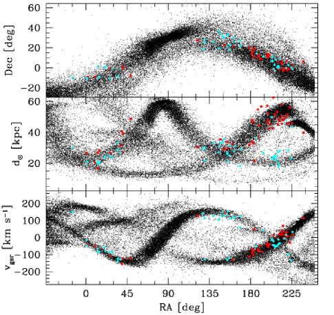
Figure 9.— The position, heliocentric distance, and galactocentric velocity of the Law & Majewski (2010) Sagittarius $N$-body model (black dots) and the blue horizontal branch (red squares) and blue stragglers (cyan diamonds) that match the Sagittarius $N$-body model in position, velocity, and distance.

4.1. Stellar Populations and Sagittarius $N$-body Models

Law & Majewski (2010) construct and analyze a sophisticated $N$-body model of the evolution of Sagittarius in a triaxial Milky Way potential. The model matches all existing observational constraints on the nature of the dwarf galaxy and the streams of debris, providing a benchmark for interpreting the apparent debris streams we detect in the HVS survey.

We test the positions and radial velocities of HVS sample stars in the 25 most significant great circles against the Law & Majewski (2010) model. Figure 9 shows the position, heliocentric distance, and galactocentric velocity for the Law & Majewski (2010) $N$-body model (black dots).

Brown et al. (2010) compute luminosity estimates for each star in the HVS survey by matching observed colors and spectroscopy to stellar evolution tracks for metal-poor main sequence (Girardi et al., 2002, 2004) and post-main sequence (Dotter et al., 2007, 2008) stars. Coupled with the Law & Majewski (2010) model, these luminosities enable us to discriminate between blue stragglers and BHB stars in the HVS survey.

BHB stars in the HVS survey have a mean $M_{g}=1.15\pm 0.35$; blue stragglers have a mean $M_{g}=2.25\pm 0.45$ (Brown et al., 2010). Thus, blue stragglers should sample the nearest regions of the Sagittarius stream; BHB stars should sample the furthest regions. Both types of stars contribute to the stream for distances $20<d<45$ kpc.

Of the 417 stars contained in the 25 most significant great circles, 60 (14%) match the Sagittarius $N$-body model in position, velocity, and distance for a BHB star (red squares in Figure 9); 51 (12%) match the Sagittarius $N$-body model in position, velocity, and distance for a blue stragglers (cyan squares in Figure 9). Seventeen stars are common to both matches. Thus 22.5% of the stars in our 25 most significant great circles, roughly 10% of the total HVS survey sample, probably belong to the Sagittarius stream. Because some stars in the Sagittarius stream might lie in other great circles, this estimate yields a rough lower limit to the fraction of HVS survey stars within the Sagittarius stream.

The HVS survey stars that match the Sagittarius stream $N$-body model in the region $0{{}^{\circ}}<$ $RA$ $<50{{}^{\circ}}$ are an equal mix of blue stragglers and BHB stars. The stars that match the Sagittarius stream in the region $130{{}^{\circ}}<RA<180{{}^{\circ}}$ are a 2:1 mix of blue stragglers and BHB stars (Figure 9). The HVS survey fairly samples both stellar populations within the Sagittarius stream in these regions. The observations thus support the idea that the stellar population varies along the stream.

From color-magnitude diagrams of Sagittarius, Niederste-Ostholt et al. (2010) find equal numbers of blue stragglers and BHB stars in the region $150{{}^{\circ}}<$ $RA<10{{}^{\circ}}$. Detailed star count analyses, however, suggest a variation in the number ratio of BHB stars to main sequence turn-off stars along the stream (e.g., Bell et al., 2010). Our analysis is also consistent with changes in the stellar population along the stream. Bell et al. (2010) propose that Sagittarius once had a BHB-rich core and a BHB-poor halo. Population variations then result from stripping different regions of the progenitor at different times (see also, Martínez-Delgado et al., 2004; Bellazzini et al., 2006; Chou et al., 2007; Peñarrubia et al., 2010; Carlin et al., 2011). Because our analysis yields matches to the position and velocity of two stellar populations, blue stragglers and BHB stars, our results support and extend the conclusion of Bell et al. (2010) that the stellar population in the Sagittarius dwarf varied with radius prior to disruption.

4.2. Density of Blue Stars in the Sagittarius Stream

The Law & Majewski (2010) model sets a rough lower limit on the contribution of Sagittarius to the HVS survey population. From the observed data, we derive an approximate upper limit. To make this estimate, we compute great circle counts for widths, $\Delta$, between 1^∘ and 20^∘. For each $\Delta$, we perform the analysis outlined in §2 and identify the great circle with the smallest $p_{Joint}$. We then compare the number of stars within this great circle, $n_{obs}$, with the number expected, $n_{exp}$, for a random distribution of stars on the sky. The estimated number of stars within the Sagittarius stream is the excess number of stars above random, $n_{Sgr}$ = $n_{obs}-n_{exp}$. A posteriori, we verify that the locations of the poles for this collection of great circles change little as a function of $\Delta$ and that the excess number of stars as a function of $\Delta$ is independent of any small change in the $(l,b)$ of the most significant pole for an adopted $\Delta$.

Figure 10 shows our estimate for the number of survey stars in the Sagittarius stream, $n_{Sgr}$, as a function of $\Delta$. The derived $n_{Sgr}$ rises from $\sim$ 70 for $\Delta=5{{}^{\circ}}$ to $\sim$ 150 for $\Delta$ = 14^∘ and then levels off. Adopting a typical $n_{Sgr}\approx 150$ for $\Delta$ = 14^∘–20^∘, this result implies that roughly 17% (150 stars out of 881) in the HVS survey sample belong to the Sagittarius stream. This estimate is larger than the $\sim$ 10% derived from the comparison of our 25 most significant great circles with the Law & Majewski (2010) model in §4.1. Combining these results shows that Sagittarius contributes about 10% to 17% of the stars in the HVS survey.

Because this approach uses the full HVS survey, it yields a better estimate of the fraction of HVS survey stars within the Sagittarius stream.

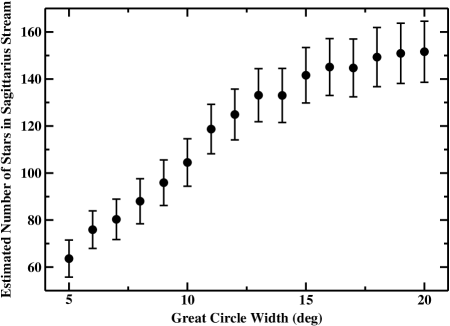
Figure 10.— Estimated number of stars from the HVS survey within Sagittarius as a function of great circle width $\Delta$.

4.3. Stellar Surface Density of the Sagittarius Stream

To conclude this section, we compare the surface density of stars identified in our observations of the Sagittarius stream with the predictions of the Law & Majewski (2010) model. For each iteration in a Monte Carlo simulation, we construct a sample of model stars with the same number of stars observed in the HVS survey. This model sample consists of (i) stars drawn randomly from the Law & Majewski (2010) model and (ii) stars distributed randomly and isotropically in the HVS survey area. Based on our result in §4.2, we select 17% of this sample from the Law & Majewski (2010) model. We then analyze great circle counts using the same procedure as for the HVS survey sample with $\Delta=5{{}^{\circ}}$. Repeating this process $200$ times, we derive the median value of $p_{GC}$ for the most significant pole in the model Sagittarius stream.

Using equation 1, we can express the ratio of the observed surface density to that predicted from the Monte Carlo simulations as $\gamma=\frac{n_{obs}p_{MC}}{n_{MC}p_{obs}}$. Here, $n_{obs}$ is the number of stars in the most significant great circle observed in the HVS survey sample, $n_{MC}$ is the median value of the number of stars in the most significant great circle from the Monte Carlo simulations, and $p_{obs}$ and $p_{MC}$ are, respectively, the probabilities that a star placed randomly in the sample region falls within the observed or simulated great circle.

This analysis shows that the Law & Majewski (2010) model matches our observed surface density for stars in the Sagittarius stream. For simulations with $\Delta$ = 5^∘, we derive $\gamma$ = 1.03, with a 90% confidence interval of 0.82–1.43. Simulations with other $\Delta$’s yield similar results.

5. CONCLUSION

We construct a statistical technique to detect star streams in the Galactic halo based on both the surface number density and the radial velocity distribution within great circles. The addition of radial velocities to the analysis increases our ability to identify star streams and to show that some overdensities in number counts are superpositions of several distinct structures in velocity space. The technique is straightforward yet powerful, can be generalized to diverse sets of data, and quantifies the statistical significance of tidal star streams. Detection is possible even when a structure contributes only a few percent of the stars in a sample.

We apply the method to the HVS survey and detect the Sagittarius stream at high significance. Comparison with theoretical models confirms that blue stragglers and BHB stars are members of the Sagittarius stream. Great circle counts and comparisons with theoretical models suggest that the Sagittarius stream comprises 10% to 17% of the halo stars in the HVS sample. The ratio of blue stragglers to blue horizontal branch stars varies along the length of the stream, with roughly equal numbers of these two stellar types at RA = 0^∘–50^∘ and a 2:1 mix of blue stragglers to blue horizontal branch stars at RA = 130^∘–180^∘. Our conclusions support previous indications of variations in stellar population related to the original structure of the dwarf galaxy.

This technique is easily applied to other large radial velocity surveys including RAVE (Steinmetz et al., 2006; Zwitter et al., 2008) and SEGUE (Yanny et al., 2009). Identifying tidal star streams in these radial velocity surveys will ultimately improve constraints on the Milky Way’s formation history, dark matter halo mass distribution, and the distributions of stellar populations within the progenitors.

Table 1The 25 Most Significant Poles Ranked by $p_{Joint}^{adjusted}$

$l$ (deg)	$b$ (deg)	Rank	$p_{GC}$	$p_{V_{rf}}$	$p_{Joint}$	$p_{GC}^{adjusted}$	$p_{Joint}^{adjusted}$
Sagittarius Stream – Branch A
101.0	16.3	3	$2.29\times 10^{-12}$	$1.11\times 10^{-01}$	$2.56\times 10^{-13}$	$2.27\times 10^{-08}$	$2.53\times 10^{-09}$
101.6	15.0	16	$9.44\times 10^{-11}$	$1.62\times 10^{-01}$	$1.53\times 10^{-11}$	$9.33\times 10^{-07}$	$1.51\times 10^{-07}$
102.4	16.3	11	$6.61\times 10^{-11}$	$4.77\times 10^{-02}$	$3.16\times 10^{-12}$	$6.54\times 10^{-07}$	$3.12\times 10^{-08}$
103.1	12.4	1	$3.67\times 10^{-13}$	$1.28\times 10^{-01}$	$4.69\times 10^{-14}$	$3.63\times 10^{-09}$	$4.63\times 10^{-10}$
103.7	16.3	19	$5.05\times 10^{-10}$	$4.92\times 10^{-02}$	$2.49\times 10^{-11}$	$4.99\times 10^{-06}$	$2.46\times 10^{-07}$
103.9	13.7	9	$1.35\times 10^{-11}$	$1.89\times 10^{-01}$	$2.56\times 10^{-12}$	$1.34\times 10^{-07}$	$2.53\times 10^{-08}$
104.3	15.0	24	$6.05\times 10^{-10}$	$1.17\times 10^{-01}$	$7.08\times 10^{-11}$	$5.98\times 10^{-06}$	$7.00\times 10^{-07}$
104.5	12.4	2	$5.05\times 10^{-13}$	$2.18\times 10^{-01}$	$1.10\times 10^{-13}$	$4.99\times 10^{-09}$	$1.09\times 10^{-09}$
105.3	13.7	6	$1.47\times 10^{-11}$	$1.12\times 10^{-01}$	$1.65\times 10^{-12}$	$1.45\times 10^{-07}$	$1.63\times 10^{-08}$
106.6	13.7	15	$4.69\times 10^{-11}$	$2.85\times 10^{-01}$	$1.34\times 10^{-11}$	$4.63\times 10^{-07}$	$1.32\times 10^{-07}$
Associated with Sagittarius Stream – Branch A
96.9	16.3	21	$2.55\times 10^{-10}$	$1.19\times 10^{-01}$	$3.04\times 10^{-11}$	$2.52\times 10^{-06}$	$3.01\times 10^{-07}$
99.6	16.3	4	$2.18\times 10^{-12}$	$3.17\times 10^{-01}$	$6.91\times 10^{-13}$	$2.15\times 10^{-08}$	$6.83\times 10^{-09}$
100.2	15.0	25	$7.93\times 10^{-10}$	$9.01\times 10^{-02}$	$7.15\times 10^{-11}$	$7.84\times 10^{-06}$	$7.07\times 10^{-07}$
101.8	12.4	8	$3.13\times 10^{-11}$	$7.12\times 10^{-02}$	$2.23\times 10^{-12}$	$3.09\times 10^{-07}$	$2.20\times 10^{-08}$
105.8	12.4	10	$1.02\times 10^{-11}$	$2.70\times 10^{-01}$	$2.76\times 10^{-12}$	$1.01\times 10^{-07}$	$2.73\times 10^{-08}$
Associated with Sagittarius Stream
82.5	15.0	20	$9.98\times 10^{-10}$	$2.61\times 10^{-02}$	$2.60\times 10^{-11}$	$9.86\times 10^{-06}$	$2.57\times 10^{-07}$
83.9	15.0	13	$4.20\times 10^{-10}$	$1.35\times 10^{-02}$	$5.67\times 10^{-12}$	$4.15\times 10^{-06}$	$5.60\times 10^{-08}$
89.3	15.0	12	$2.43\times 10^{-09}$	$1.47\times 10^{-03}$	$3.56\times 10^{-12}$	$2.40\times 10^{-05}$	$3.52\times 10^{-08}$
90.7	15.0	18	$7.70\times 10^{-09}$	$3.08\times 10^{-03}$	$2.37\times 10^{-11}$	$7.61\times 10^{-05}$	$2.34\times 10^{-07}$
91.4	16.3	22	$1.99\times 10^{-08}$	$2.79\times 10^{-03}$	$5.55\times 10^{-11}$	$1.96\times 10^{-04}$	$5.48\times 10^{-07}$
Superpositions with Sagittarius
121.6	20.2	5	$1.12\times 10^{-12}$	$9.97\times 10^{-01}$	$1.11\times 10^{-12}$	$1.10\times 10^{-08}$	$1.10\times 10^{-08}$
122.1	18.9	23	$1.29\times 10^{-10}$	$4.88\times 10^{-01}$	$6.31\times 10^{-11}$	$1.28\times 10^{-06}$	$6.24\times 10^{-07}$
124.9	30.7	7	$2.14\times 10^{-10}$	$1.01\times 10^{-02}$	$2.16\times 10^{-12}$	$2.11\times 10^{-06}$	$2.14\times 10^{-08}$
126.4	30.7	14	$5.21\times 10^{-10}$	$1.75\times 10^{-02}$	$9.12\times 10^{-12}$	$5.15\times 10^{-06}$	$9.01\times 10^{-08}$
131.0	30.7	17	$1.21\times 10^{-09}$	$1.67\times 10^{-02}$	$2.01\times 10^{-11}$	$1.19\times 10^{-05}$	$1.99\times 10^{-07}$

References

- Abadi et al. (2003) Abadi, M. G., Navarro, J. F., Steinmetz, M., & Eke, V. R. 2003, ApJ, 597, 21
- Abdi (2007) Abdi, H. 2007, in Encyclopedia of Measurement and Statistics, ed. N. Salkind (Thousand Oaks, CA: Sage), http://www.utdallas.edu/$∼$herve/Abdi-Bonferroni2007-pretty.pdf
- Bell et al. (2010) Bell, E. F., Xue, X. X., Rix, H.-W., Ruhland, C., & Hogg, D. W. 2010, AJ, 140, 1850
- Bellazzini et al. (2006) Bellazzini, M., Newberg, H. J., Correnti, M., Ferraro, F. R., & Monaco, L. 2006, A&A, 457, L21
- Belokurov et al. (2006) Belokurov, V., et al. 2006, ApJ, 642, L137
- Brown et al. (2009a) Brown, W. R., Geller, M. J., & Kenyon, S. J. 2009a, ApJ, 690, 1639
- Brown et al. (2009b) Brown, W. R., Geller, M. J., Kenyon, S. J., & Bromley, B. C. 2009b, ApJ, 690, L69
- Brown et al. (2010) Brown, W. R., Geller, M. J., Kenyon, S. J., & Diaferio, A. 2010, AJ, 139, 59
- Brown et al. (2005) Brown, W. R., Geller, M. J., Kenyon, S. J., & Kurtz, M. J. 2005, ApJ, 622, L33
- Brown et al. (2006a) —. 2006a, ApJ, 640, L35
- Brown et al. (2006b) —. 2006b, ApJ, 647, 303
- Brown et al. (2007a) Brown, W. R., Geller, M. J., Kenyon, S. J., Kurtz, M. J., & Bromley, B. C. 2007a, ApJ, 660, 311
- Brown et al. (2007b) —. 2007b, ApJ, 671, 1708
- Bullock & Johnston (2005) Bullock, J. S., & Johnston, K. V. 2005, ApJ, 635, 931
- Carlin et al. (2011) Carlin, J. L., Majewski, S. R., Casetti-Dinescu, et al. 2011, ApJ, accepted
- Chou et al. (2007) Chou, M.-Y., Majewski, S. R., Cunha, K., et al. 2007, ApJ, 670, 346
- Dehnen & Binney (1998) Dehnen, W., & Binney, J. J. 1998, MNRAS, 298, 387
- Dotter et al. (2007) Dotter, A., Chaboyer, B., Jevremović, D., et al. 2007, AJ, 134, 376
- Dotter et al. (2008) Dotter, A., Chaboyer, B., Jevremović, D., et al. 2008, ApJS, 178, 89
- Font et al. (2006) Font, A. S., Johnston, K. V., Bullock, J. S., & Robertson, B. E. 2006, ApJ, 638, 585
- Girardi et al. (2002) Girardi, L., Bertelli, G., Bressan, et al. A. 2002, A&A, 391, 195
- Girardi et al. (2004) Girardi, L., Grebel, E. K., Odenkirchen, M., & Chiosi, C. 2004, A&A, 422, 205
- Harding et al. (2001) Harding, P., Morrison, H. L., Olszewski, E. W., et al. 2001, AJ, 122, 1397
- Ibata et al. (2001) Ibata, R., Lewis, G. F., Irwin, M., Totten, E., & Quinn, T. 2001, ApJ, 551, 294
- Ibata et al. (1994) Ibata, R. A., Gilmore, G., & Irwin, M. J. 1994, Nature, 370, 194
- Ibata et al. (2002) Ibata, R. A., Lewis, G. F., Irwin, M. J., & Cambrésy, L. 2002, MNRAS, 332, 921
- Johnston et al. (1996) Johnston, K. V., Hernquist, L., & Bolte, M. 1996, ApJ, 465, 278
- Johnston et al. (1999) Johnston, K. V., Majewski, S. R., Siegel, M. H., Reid, I. N., & Kunkel, W. E. 1999, AJ, 118, 1719
- Koay (2011) Koay, C. G. 2011, Journal of Computational Science, in press
- Law & Majewski (2010) Law, D. R., & Majewski, S. R. 2010, ApJ, 714, 229
- Lynden-Bell & Lynden-Bell (1995) Lynden-Bell, D., & Lynden-Bell, R. M. 1995, MNRAS, 275, 429
- Majewski et al. (2003) Majewski, S. R., Skrutskie, M. F., Weinberg, M. D., & Ostheimer, J. C. 2003, ApJ, 599, 1082
- Majewski et al. (2004) Majewski, S. R., Ostheimer, J. C., Rocha-Pinto, H. J., et al. 2004, AJ, 128, 245
- Martínez-Delgado et al. (2004) Martínez-Delgado, D., Gómez-Flechoso, M. Á., Aparicio, A., & Carrera, R. 2004, ApJ, 601, 242
- Newberg et al. (2007) Newberg, H. J., Yanny, B., Cole, et al. 2007, ApJ, 668, 221
- Niederste-Ostholt et al. (2010) Niederste-Ostholt, M., Belokurov, V., Evans, N. W., & Peñarrubia, J. 2010, ApJ, 712, 516
- Peñarrubia et al. (2010) Peñarrubia, J., Belokurov, V., Evans, N. W., et al. 2010, MNRAS, 408, L26
- Press et al. (1992) Press, W., Teukolsky, S., Vetterling, W., & Flannery, B. 1992, Numerical Recipes in FORTRAN, 2nd edn. (Cambridge, UK: Cambridge University Press)
- Ruhland et al. (2011) Ruhland, C., Bell, E. F., Rix, H., & Xue, X. 2011, ApJ, 731, 119
- Schlaufman et al. (2009) Schlaufman, K. C., Rockosi, C. M., Allende Prieto, C., et al. 2009, ApJ, 703, 2177
- Sharma et al. (2011) Sharma, S., Johnston, K. V., Majewski, S. R., Bullock, J., & Muñoz, R. R. 2011, ApJ, 728, 106
- Starkenburg et al. (2009) Starkenburg, E., Helmi, A., Morrison, H. L., et al. 2009, ApJ, 698, 567
- Steinmetz et al. (2006) Steinmetz, M., Zwitter, T., Siebert, A., et al. 2006, AJ, 132, 1645
- Vivas et al. (2008) Vivas, A. K., Jaffé, Y. L., Zinn, R., et al. 2008, AJ, 136, 1645
- Xue et al. (2011) Xue, X.-X., Rix, H.-W., Yanny, B., et al. 2011, ApJ, 738, 79
- Yanny et al. (2009) Yanny, B., Newberg, H. J., Johnson, J. A., et al. 2009, ApJ, 700, 1282
- Zwitter et al. (2008) Zwitter, T., Siebert, A., Munari, U., et al. 2008, AJ, 136, 421