The Extremely High-Velocity Outflow from the Luminous Young Stellar Object G5.89$-$0.39

Abstract

We have imaged the extremely high-velocity outflowing gas in CO (2$-$1) and (3$-$2) associated with the shell-like ultracompact H II region G5.89$-$0.39 at a resolution of $\sim$3$\arcsec$ (corresponding to $\sim$4000 AU) with the Submillimeter Array. The integrated high-velocity ($\gtrsim$45 km s^-1) CO emission reveals at least three blueshifted lobes and two redshifted lobes. These lobes belong to two outflows, one oriented N-S, the other NW-SE. The NW-SE outflow is likely identical to the previously detected Br$\gamma$ outflow. Furthermore, these outflow lobes all clearly show a Hubble-like kinematic structure. For the first time, we estimate the temperature of the outflowing gas as a function of velocity with the large velocity gradient calculations. Our results reveal a clear increasing trend of temperature with gas velocity. The observational features of the extremely high-velocity gas associated with G5.89$-$0.39 qualitatively favor the jet-driven bow shock model.

1 Introduction

Although molecular outflows have been commonly identified around both low- and high-mass young stellar objects (YSOs) (e.g., Bachiller & Tafalla, 1999; Arce et al., 2007), it is not clear how the bulk of the outflowing gas is accelerated. Past observations show that molecular outflows can often be divided into two components — the “classical” less-collimated component with low-velocity and the highly collimated component with extremely high-velocity (50$-$150 km s^-1, hereafter EHV) (Bachiller & Tafalla, 1999; Hirano et al., 2006; Palau et al., 2006). Exploring the physical conditions of the EHV molecular gas in details will be helpful for clarifying its role in star formation processes.

The massive star forming region G5.89$-$0.39 (hereafter G5.89) is associated with energetic CO outflows with velocities up to $\sim$$\pm$70 km s^-1 from its systemic velocity, among the highest gas velocities that have been detected in molecular outflows (e.g., Choi et al., 1993). G5.89 also harbors a shell-like ultracompact (UC) H II region powered by a young O-type star (hereafter Feldt’s star) visible in the near-IR (Wood & Churchwell, 1989; Feldt et al., 2003). Based on the deduced gas temperature structure, Su et al. (2009) conclude that Feldt’s star supplies the majority of energy for heating the dense gas enshrouding the UC H II region.

The outflowing gas associated with G5.89 was first identified by Harvey & Forveille (1988) in CO (1$-$0) with the IRAM 30-m telescope. Subsequent studies reported outflows with notably different orientations in various tracers. For example, SiO (5$-$4) observations with the Submillimeter Array (SMA) resolved a bipolar structure along a position angle (P.A.) of $\sim$30^∘ (Sollins et al., 2004). On the other hand, sub-arcsecond CO (3$-$2) images made with the SMA (Hunter et al., 2008) detected a well-collimated N-S outflow and tentatively a compact NW-SE outflow associated with the Br$\gamma$ outflow revealed by Puga et al. (2006). Both CO outflows demonstrate EHV gas, with velocities $\gtrsim$50 km s^-1. Furthermore, BIMA observations in CO (1$-$0) and HCO⁺ (1$-$0) identified an outflow along the E-W direction (Watson et al., 2007). These results imply the existence of multiple YSOs toward G5.89. Indeed, five sub-mm dust sources (denoted as SMA1, SMA2, SMA-N, SMA-E, and SMA-S) were located in the close vicinity of the UC H II region G5.89 (Hunter et al., 2008).

Here we present SMA observations of G5.89 in CO (2$-$1) and (3$-$2) at resolutions of $\sim$3$\arcsec$. We perform large velocity gradient (LVG) calculations to explore the physical conditions of the EHV outflowing gas. We then discuss the nature of the EHV components and their connection to the gas accelerating processes.

2 Observations and Data Reduction

The observations were carried out with the SMA on 2008 April 17 and May 2 in the band of 230 GHz, and on 2006 July 27 and September 10 in the band of 345 GHz. The phase center was R.A. = 18^h00^m30.32^s (J2000) and decl. = $-$24°04′00.50$\arcsec$ (J2000). At 230 GHz band, CO (2$-$1) was observed with seven antennas in the compact configuration, which resulted in projected baselines ranging from about 9 m to 120 m (7 to 90 k$\lambda$). For the CO (3$-$2) observations at 345 GHz band with also seven antennas in the compact configuration, the projected baselines ranged from about 9 m to 70 m (10 to 80 k$\lambda$). The half-power width of the SMA primary beam was $\sim$51$\arcsec$ at 230 GHz and $\sim$34$\arcsec$ at 345 GHz. The total available double-sideband bandwidth was 4 GHz. The spectral resolutions of 230 GHz and 345 GHz observations were 0.41 MHz (0.53 km s^-1) and 0.81 MHz (0.71 km s^-1), respectively. See Ho, Moran, & Lo (2004) for more complete specifications of the SMA.

For the 345 GHz band observations, the flux calibrator was Uranus and the bandpass calibrators were Uranus (July 27 and September 10), Callisto (July 27), and 3C279 (September 10). The nearby compact radio sources 1626$-$298 (S $\sim$ 2.2 Jy in July 27 and 1.8 Jy in September 10) and 1924$-$292 (S $\sim$ 3.4 Jy in July 27 and 2.9 Jy in September 10) served as complex gain calibrators. See Su et al. (2009) for the calibration information of the 230 GHz band observations. For both 230 GHz and 345 GHz band observations, the absolute flux density scales were estimated to have an uncertainty of $\sim$20% . We calibrated the data using the MIR software package adapted for the SMA from the software package developed originally for the OVRO MMA (Scoville et al., 1993). We made maps using the MIRIAD package (Sault et al., 1995). With robust weighting, the synthesized beam size was about 3.2$\arcsec$ $\times$ 2.4$\arcsec$ at P.A. of 40.8^∘ for the CO (2$-$1) maps, and about 3.0$\arcsec$ $\times$ 2.0$\arcsec$ at P.A. of 13.5^∘ for the CO (3$-$2) maps. We smoothed our data to 2.0 km s^-1 resolution for the analysis presented below. The rms noise level in a 2.0 km s^-1 velocity bin is $\sim$35 mJy beam^-1 ($\sim$0.10 K) at 230 GHz and $\sim$90 mJy beam^-1 ($\sim$0.15 K) at 345 GHz.

3 CO (2$-$1) & (3$-$2) Emissions

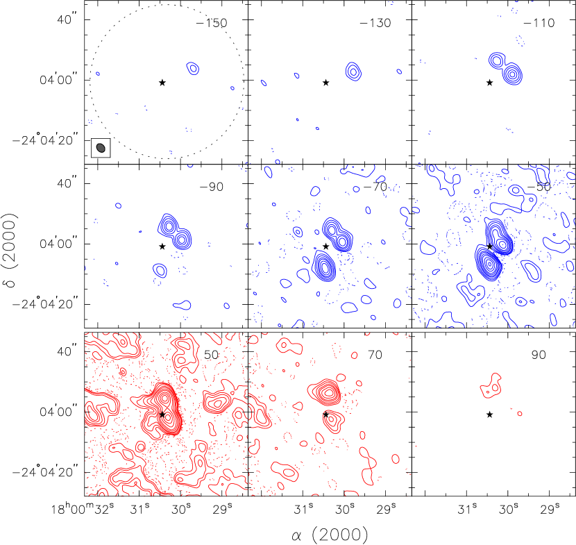
Figure 1: Channel maps of G5.89$-$0.39 in CO (2$-$1) emission at high velocity. The local standard of rest velocity of each channel’s center is indicated in the upper right corner of each panel. The LSR velocity of the system is about $+$9.0 km s^-1. Solid contours are at 4, 10, 20, 40, 60, 100, 150, 250, 350, and 450 $\times$ $\sigma$, and dotted contours indicate $-$4, $-$10, $-$20, $-$40, and $-$60 $\times$ $\sigma$, where $\sigma$ = 11 mJy beam^-1. The dotted circle shown in the first panel represents the primary beam of the SMA observations. The synthesized beam is shown in the lower left corner of the first panel. The asterisk represents the position of the H II region powering star, i.e., Feldt’s star (Feldt et al., 2003).

Figure 1 shows channel maps of the blueshifted and redshifted CO (2$-$1) emissions associated with G5.89. For display purposes, we have smoothed the channel maps to a velocity resolution of 20.0 km s^-1. The spatial distributions of CO (2$-$1) and (3$-$2) agree with each other very well, and the velocity extents of the CO (2$-$1) and (3$-$2) outflows are comparable. Emissions are detected to velocities $v_{flow}$ $\approx$ 80 km s^-1 in the redshifted lobes and $v_{flow}$ $\approx$ 160 km s^-1 in the blueshifted lobes, where $v_{flow}$ $\equiv$ $|V_{flow}-V_{lsr}|$ with $V_{flow}$ being the apparent outflow velocity and $V_{lsr}$ (= $+$9.0 km s^-1) the systemic velocity of G5.89. The EHV line wing detected here is significantly broader than that reported by single-dish observations (e.g., Choi et al., 1993). The difference is due to the relatively poor sensitivities of single-dish observations. The structure of the CO gas with $v_{flow}$ $\lesssim$ 40 km s^-1 is extended and complex. Due to the lack of short-spacing data to recover the extended structure filtered out by our SMA observations, in Figure 1 the low-velocity components are excluded.

The left and right panels of Figure 2 show the integrated blueshifted and redshifted emissions of CO (2$-$1) and (3$-$2), respectively. For both transitions, the emissions are integrated over the line wing, with 50 $\lesssim$ $v_{flow}$ $\lesssim$ 162 km s^-1 for the blueshifted gas and 42 $\lesssim$ $v_{flow}$ $\lesssim$ 80 km s^-1 for the redshifted gas. The outflow morphologies seen in CO (2$-$1) and (3$-$2) are very similar. Although only EHV line wing is integrated, the morphology of the EHV gas is complicated — at least three bluedshifted lobes (denoted as B-N lobe, B-NW lobe, and B-S lobe) and two redshifted lobes (denoted as R-N lobe and R-S lobe) are revealed in the vicinity of the UC H II region G5.89. There appears to be an additional redshifted lobe located $\sim$4″  southeast to Feldt’s star.

Both B-S lobe and R-N lobe have been identified by previous SMA CO (3$-$2) observations at sub-arcsecond resolution, and were proposed to be a pair of the N-S bipolar outflow driven by the sub-mm dust source SMA1 (Hunter et al., 2008). The authors also proposed a second CO outflow along P.A. about $-$55^∘ associated with the Br$\gamma$ outflow reported by Puga et al. (2006). Our observations confirm the existence of this NW-SE outflow, consisting of the B-NW lobe and R-S lobe. The B-N lobe was also identified by Hunter et al. (2008), although its driving source is less clear. The existence of the B-N lobe could be explained by the N-S outflow being close to the plane of the sky, but this is very unlikely from the kinematic viewpoint. After correcting for projection, the N-S outflow, if in the plane of sky, will have molecular gas with velocity up to $>$500 km s^-1, about a factor of 3 higher than the highest gas velocities that ever identified in molecular outflows. Figure 3 shows the position-velocity (P-V) diagrams of the CO (2$-$1) and (3$-$2) along P.A. 175^∘ (left panel) centered on the dust source SMA1 and 130^∘ (right panel) centered on the dust source SMA2. The Hubble-like kinematic feature, i.e., the outflow velocity increasing with the distance from the central YSO, is clearly discerned in both outflows with a velocity gradient about 1000 km s^-1 pc^-1.

Assuming an inclination of 45^∘ and a distance of 1.28 kpc (Motogi et al., 2011), the inferred dynamical timescales range from 400 years to 650 years. Since the axes of these outflows are unlikely close to either the plane of the sky or the line of sight, the derived dynamical timescales should be accurate to within a factor of 3$-$4. The observed outflow lobes therefore represent the most recent outflow activities in this region.

4 Line Ratios & Excitation Conditions of the Outflowing Gas

Given the fairly good signal-to-noise ratio of the CO emission detected toward G5.89 even at EHV line wing, it is feasible to estimate the physical parameters with a relative narrow velocity bin (10 km s^-1) and investigate their velocity-dependence. Table 1 summarizes the observed CO (2$-$1) intensities (in brightness temperature scale) as well as the intensity ratios of CO (3$-2$) and (2$-$1) as a function of gas velocity for all the observed lobes.

For a proper comparison, both CO (2$-$1) and (3$-$2) maps were reconstructed with a clean beam of 3.4$\arcsec$ in order to match the resolutions. For each velocity bin, furthermore, we simply report the value calculated from the CO (2$-$1) peak toward each lobe rather than the value averaged over entire lobe to avoid the difficulty of emission separation from various lobes, in particular, at relatively low-velocity channels. We emphasize that for each outflow lobe, the peak positions of CO (2$-$1) and (3$-$2) in various velocity bins agree very well with each other, with both median and mean offsets of $\sim$0.25$\arcsec$, and no systematic offsets can be discerned. Consequently we do not expect any systematic bias for the physical conditions estimated afterward. As listed in Table 1, most deduced line ratios are in the range of 0.6$-$1.2.

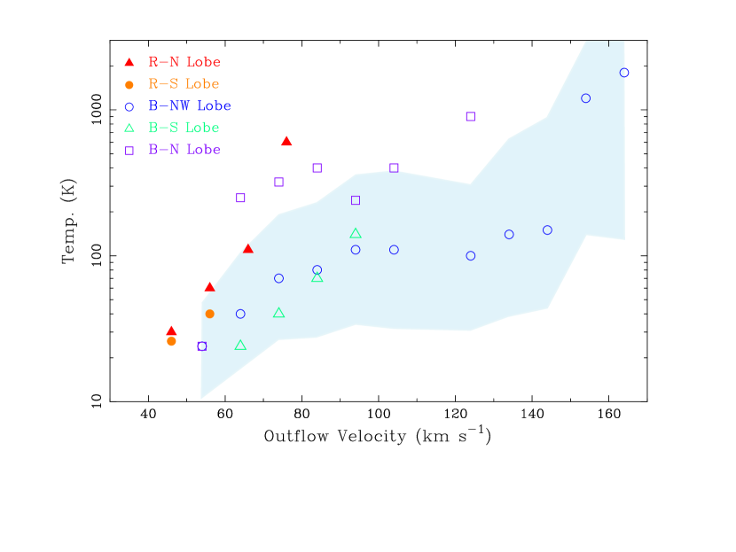
Figure 4: Temperature of the outflowing gas deduced from the LVG calculations versus the corresponding gas velocity. An increasing trend of gas temperature with outflow velocity can be discerned toward all lobes. The blue-shaded area represents the 1-$\sigma$ temperature uncertainty when allowing flux variations up to 20% in the B-NW lobe. Note that the outflow velocity $v_{flow}$ shown here is related to the velocity $V_{flow}$ listed in Table 1 by the relation: $v_{flow}$ = $|V_{flow}-V_{lsr}|$ with $V_{lsr}$ = $+$9.0 km s^-1 the systemic velocity of G5.89$-$0.39. The lobes of N-S and NW-SE outflows are represented by triangles and circles, respectively.

To estimate the physical conditions of the outflowing gas, we performed the LVG analysis with the code written by L. G. Mundy and implemented as part of the MIRIAD package (Sault et al., 1995). We assumed the canonical CO fractional abundance of 10^-4 and a velocity gradient of 1000 km s^-1 pc^-1 as estimated from the Hubble-like kinematic structure (in Figure 3). Figure 4 shows the gas temperature estimated from the LVG calculations versus gas velocity. The plot exhibits a clear increasing trend of gas temperature with outflow velocity. Such a trend can be discerned toward all the lobes, although the trend of the B-N lobe is less clear. In the case of B-NW lobe, there appears to be a temperature jump at outflow velocities of $\sim$150 km s^-1, with gas temperature ranging from 1200$-$1800 K for v_flow $\gtrsim$150 km s^-1 and $\lesssim$150 K for v_flow $\lesssim$150 km s^-1. The estimated temperature of the above highest-velocity bins in the B-NW lobe will be reduced to 400$-$500 K hence eliminating the above-mentioned temperature jump if the assumed CO fractional abundance is lowered by a factor of 2. The occurrence of abundance reduction may be attributed to partial dissociation or even ionization of CO molecules under high-excitation conditions.

A few factors may contribute to the uncertainty of the temperature estimates reported above. Given the flux calibration uncertainty of 20%, the gas temperature obtained with LVG calculations would vary by a factor of 10 or so. In Figure 4, we show with the blue-shaded area the 1-$\sigma$ temperature range when allowing flux variations up to 20% in the B-NW lobe. Although the temperature uncertainty appears fairly large, we emphasize that the general increasing trend of gas temperature with outflow velocity is indeed robust. For a given flux calibration error, the line ratios will be affected in the same way in all channels and render a simple temperature shift across all velocity bins. For the LVG calculations, variations in input parameters also lead to variations in the derived temperature by a similar factor and hence do not change the general increasing trend on temperature with gas velocity. For example, the derived temperature will decrease by about a factor of 3 if the adopted CO fractional abundance is reduced by half or the velocity gradient increases twice. Although variation in velocity gradient or CO abundance across the line wings could mimic the derived temperature trend with velocity, the Hubble-like kinematic feature shown in Figure 3 makes this confusion quite unlikely. A precise gas temperature estimate will need observations with better flux calibration. Alternatively, observations in higher transitions of CO will also help to constrain hot gas temperature.

5 The Origin of the EHV Components and Their Connection to the Gas Accelerating Processes

Observations have shown that the kinetic temperature of high-velocity molecular gas in outflows associated with YSOs can be as high as 100$-$1000 K. For example, the inner SiO knots in HH211 jet have a temperature excess of 300$-$500 K (Hirano et al., 2006). In the case of extremely active molecular jets in L1448-mm, the kinetic temperature of the EHV bullets close to the YSO is estimated to be $\gtrsim$ 500 K (Nisini et al., 2007). Gas temperature estimated from near-IR H₂ observations typically ranges from 1000$-$2500 K (Richer et al., 2000; Dionatos et al., 2010). Both hot H₂ emission and warm SiO bullets are thought to trace shocked molecular gas. The broad velocity dispersions revealed from the kinematic structures of the EHV bullets further indicate their connections to (bow) shocks (Lee et al., 2001; Hirano et al., 2006; Su et al., 2007).

Could the heating of the EHV gas associated with G5.89 be dominated by shocks? Indeed, shock indicators have been detected around the highest velocity gas of the N-S and NW-SE outflows (Hofner & Churchwell, 1996; Kurtz, Hofner, & Álvarez, 2004; Hunter et al., 2008; Puga et al., 2006). For example, as shown in Figure 2 the highest-velocity gas in the R-N lobe is associated with masers of H₂O and Class I CH₃OH as well as H₂ knots (labeled as C1 and C2 by Puga et al. (2006)). Furthermore, the positions of the highest velocity gas detected in the B-NW and B-S lobes coincide with the H₂ knots B and group A, respectively, very well. The highest velocity in the B-NW lobe is also associated with masers of NH₃ and Class I CH₃OH. The hot (about 150-1800 K) molecular gas in the highest-velocity bins of the N-S and NW-SE outflows can be naturally interpreted as shock-heated gas, while the lack of velocity spread in the outflow tips (Figure 3) can be attributed to insufficient sensitivity.

It is expected that the outflow driving process provides energetics to not only accelerate but also heat the (ambient) gas. Estimations made from a simple jet-driven bow shock model predict temperature rising with outflow velocity and distance from the driving source (Hatchell, Fuller & Ladd, 1999), while such trends are different from the predictions of other classes of models (Arce et al., 2007). Hatchell, Fuller & Ladd (1999) further argued that comparing with the molecular cooling mechanisms, the heating (as a consequence of acceleration) is sufficient to maintain outflowing gas temperature a few times higher than that of ambient materials. Since the Hubble-like kinematic structure can also be reproduced by the jet-driven bow shock model (Lee et al., 2001; Arce et al., 2007), all above-mentioned features of the EHV gas associated with G5.89 can be qualitatively interpreted by the jet-driven bow shock model. We note that most, if not all, available bow shock models have parameters typical of low-mass outflows. Models with physical conditions more similar to outflows from high-mass young stars will be desired to have quantitative comparisons between observational results and model predictions. Observations with better sensitivities and spatial resolutions are also essential to search for the bow shock signatures in both morphology and kinematics.

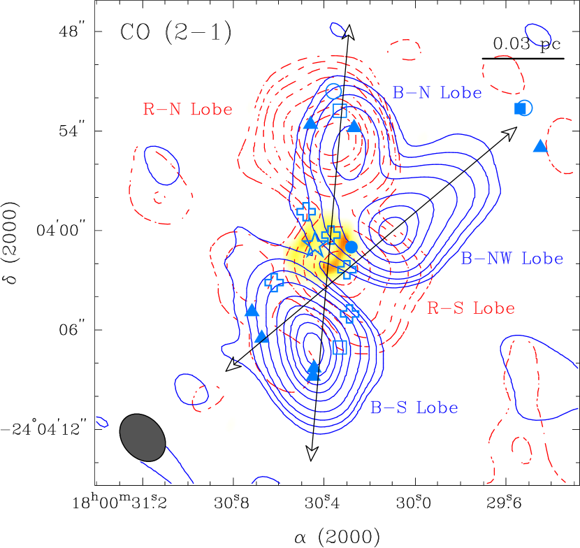
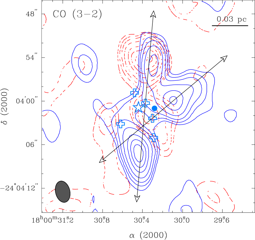
Figure 2: Extremely high-velocity molecular outflows of G5.89$-$0.39 in CO (2$-$1) (left) and (3$-$2) (right) imaged with the SMA. For both transitions, the blueshifted and redshifted lobes are integrated over the line wing, with 50 $\lesssim$ $v_{flow}$ $\lesssim$ 162 km s^-1 for the blueshifted gas and 42 $\lesssim$ $v_{flow}$ $\lesssim$ 80 km s^-1 for the redshifted gas. In the left panel, the overlaid color scales represent the free-free emission at 2 cm (Tang et al., 2009), filled triangles are the near-IR H₂ knots from Puga et al. (2006), filled square is the NH₃ maser from Hunter et al. (2008), open circles are Class I methanol maser positions (components 1 and 2 from Kurtz, Hofner, & Álvarez (2004)) and open squares are positions of water masers (components 1 and 3 from Hofner & Churchwell (1996)). In each panel, the crosses mark the position of the sub-mm dust components reported by Hunter et al. (2008), the asterisk marks the position of Feldt’s star (Feldt et al., 2003), and the filled circle labels the Br$\gamma$ outflow center (Puga et al., 2006). The synthesized beam is shown in the lower left corner. The two black lines represent the axes of the position-velocity diagrams plotted in Figure 3. In the left panel, contours are 4, 10, 20, 40, 80, 120, 160, 200, and 240 $\times$ $\sigma$, where $\sigma$ = 0.53 and 0.31 Jy beam^-1 km s^-1, respectively, for the blue- and redshifted components. In the right panel, contours are 4, 10, 20, 40, 80, 120, 160, and 200 $\times$ $\sigma$, where $\sigma$ = 1.36 and 0.80 Jy beam^-1 km s^-1, respectively, for the blueshifted and redshifted components.

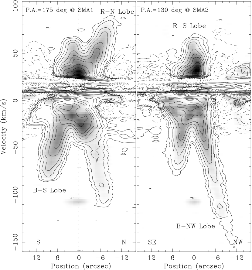
Figure 3: Position-velocity diagram of G5.89$-$0.39 in CO (2$-$1) (contours) and (3$-2$) (grayscales) along the P.A. of 175^∘ centered at SMA1 (left) and P.A. of 130^∘ centered at SMA2 (right). In each panel, the horizontal line marks the LSR velocity of the system (i.e., $+$9.0 km s^-1), and the vertical line indicates the position of SMA1 (left) and SMA2 (right).

Table 1: Observed CO (2$-$1) Intensities and CO (3$-$2)/(2$-$1) Line Ratios of the Five Outflow Lobes

BLUESHIFTED COMPONENTS							REDSHIFTED COMPONENTS
LSR Outflow	B-NW Lobe		B-N Lobe		B-S Lobe		LSR Outflow	R-N Lobe		R-S Lobe
Velocity Ranges	2$-$1a	ratiob	2$-$1a	ratiob	2$-$1a	ratiob	Velocity Ranges	2$-$1a	ratiob	2$-$1a	ratiob
(km s-1)	(K)		(K)		(K)		(km s-1)	(K)		(K)
$-$160 to $-$150	0.21	0.62	—	—	—	—	40 to 50	20.08f	0.87f	20.08f	0.87f
$-$150 to $-$140	0.41	0.73	—	—	—	—	50 to 60	13.16	1.01	8.51	0.83
$-$140 to $-$130	0.40	0.50	—	—	—	—	60 to 70	6.75	1.10	2.23	0.56
$-$130 to $-$120	0.80	0.59	0.10	1.50	—	—	70 to 80	3.73	1.05	—	—
$-$120 to $-$110	1.89	0.72	0.28	0.61	—	—	80 to 90	0.72	0.80	—	—
$-$110 to $-$100	1.49	—c	1.21	—c	—	—
$-$100 to $-$90	1.78	0.73	1.78	1.10	—	—
$-$90 to $-$80	2.04	0.78	2.29	1.07	0.81	0.60
$-$80 to $-$70	2.84	0.82	1.92	1.15	3.70	0.92
$-$70 to $-$60	3.99	0.94	2.14	1.13	6.61	0.91
$-$60 to $-$50	6.35	0.94	2.61	1.19	10.54	0.87
$-$50 to $-$40	11.08d	0.87d	11.08d	0.87d	14.41	0.84
$-$40 to $-$30	18.92e	0.84e	18.92e	0.84e	18.92e	0.84e

References

- Arce et al. (2007) Arce, H. G., Shepherd, D., Gueth, F., Lee, C.-F., Bachiller, R., Rosen, A., & Beuther, H. 2007, in Protostars and Planets V, ed. Reipurth, B., Jewitt, D. & Keil, K., (Tucson: University of Arizona Press), 245
- Bachiller & Tafalla (1999) Bachiller, R. & Tafalla M. 1999, in The Origin of Stars and Planetary Systems, ed. C. J. Lada & N. D. Kylafis (NATO ASI Ser. C, 540 Dordrecht: Kluwer), 227
- Choi et al. (1993) Choi, M., Evans, N. J., II, & Jaffe, D. T. 1993, ApJ, 417, 624
- Dionatos et al. (2010) Dionatos, O., Nisini, B., Cabrit, S., Kristensen, L., & Pineau Des Forets, G. 2010, A&A, 521, 7
- Feldt et al. (2003) Feldt, M., Puga, E., Lenzen, R. et al. 2003, ApJ, 599, L91
- Harvey & Forveille (1988) Harvey, P. M., & Forveille, T. 1988, A&A, 197, L19
- Hatchell, Fuller & Ladd (1999) Hatchell, J., Fuller, G. A., & Ladd, E. F. 1999, A&A, 344, 687
- Hirano et al. (2006) Hirano, N., Liu, S.-Y., Shang, H., Ho, P. T. P., Huang, H.-C., Kuan, Y.-J., McCaughrean, M. J., & Zhang, Q. 2006, ApJ, 636, L141
- Ho, Moran, & Lo (2004) Ho, P. T. P., Moran, J., Lo, K. Y. 2004, ApJ, 616, L1
- Hofner & Churchwell (1996) Hofner, P., & Churchwell, E. 1996, A&AS, 120, 283
- Hunter et al. (2008) Hunter, T. R., Brogan, C. L., Indebetouw, R., & Cyganowski, C. J. 2008, ApJ, 680, 1271
- Kurtz, Hofner, & Álvarez (2004) Kurtz, S., Hofner, P., & Álvarez, C. V. 2004, ApJS, 155, 149
- Lee et al. (2001) Lee, C.-F., Stone, J. M., Ostriker, E. C., & Mundy, L. G. 2001, ApJ, 557, 429
- Motogi et al. (2011) Motogi, K., Sorai, K., Habe, A., Honma, M., Kobayashi, H., & Sato, K. 2011, PASJ, 63, 31
- Nisini et al. (2007) Nisini, B., Codella, C., Giannini, T., Santiago Garcia, J., Richer, J. S., Bachiller, R., & Tafalla, M. 2007, A&A, 462, 16
- Palau et al. (2006) Palau, A., Ho, P. T. P., Zhang, Q., Estalella, R., Hirano, N., Shang, H., Lee, C.-F., Bourke, T. L., Beuther, H., & Kuan, Y.-J. 2006, ApJ, 636, 137
- Puga et al. (2006) Puga, E., Feldt, M., Alvarez, C., Henning, Th., Apai, D., Le Coarer, E., Chalabaev, A., & Stecklum, B. 2006, ApJ, 641, 373
- Richer et al. (2000) Richer, J. S., Shepherd, D. S., Cabrit, S., Bachiller, R., & Churchwell, E. 2000, Protostars and Planets IV, ed. V. Mannings, A. P. Boss, & S. S Russell (Tucson, AZ: Univ. Arizona), 867
- Sault et al. (1995) Sault, R. J., Teuben, P. J., & Wright, M. C. H. 1995, in ASP Conf. Ser. 77, Astronomical Data Analysis Software and Systems IV, ed. R. Shaw, H. E. Payne, & J. J. E. Hayes (San Francisco: ASP), 433
- Scoville et al. (1993) Scoville, N. Z., Carlstrom, J. E., Chandler, C. J., Phillips, J. A., Scott, S. L., Tilanus, R. P. J., & Wang, Z. 1993, PASP, 105, 1482
- Sollins et al. (2004) Sollins, P. K., Hunter, T. R., Battat, J. et al. 2004, ApJ, 616, L35
- Su et al. (2007) Su, Y.-N., Liu, S.-Y., Chen, H.-R., Zhang, Q. and Cesaroni, R. 2007, ApJ, 671, 571
- Su et al. (2009) Su, Y.-N., Liu, S.-Y., Wang, K.-S., Chen, Y.-H., and Chen, H.-R. 2009, ApJ, 704, L5
- Tang et al. (2009) Tang, Y.-W., Ho, P. T. P., Girart, J. M., Rao, R., Koch, P., & Lai, S.-P. 2009, ApJ, 695, 1399
- Watson et al. (2007) Watson, C., Churchwell, E., Zweibel, E. G., & Crutcher, R. M. 2007, ApJ, 657, 318
- Wood & Churchwell (1989) Wood, D. O. S., & Churchwell, E. 1989, ApJS, 69, 831