Markovian evolution of classical and quantum correlations in transverse-field $XY$ model

Abstract

The transverse-field $XY$ model in one dimension is a well-known spin model for which the ground state properties and excitation spectrum are known exactly. The model has an interesting phase diagram describing quantum phase transitions (QPTs) belonging to two different universality classes. These are the transverse-field Ising model and the $XX$ model universality classes with both the models being special cases of the transverse-field $XY$ model. In recent years, quantities related to quantum information theoretic measures like entanglement, quantum discord (QD) and fidelity have been shown to provide signatures of QPTs. Another interesting issue is that of decoherence to which a quantum system is subjected due to its interaction, represented by a quantum channel, with an environment. In this paper, we determine the dynamics of different types of correlations present in a quantum system, namely, the mutual information $I\left(\rho_{AB}\right)$, the classical correlations $C\left(\rho_{AB}\right)$ and the quantum correlations $Q\left(\rho_{AB}\right)$, as measured by the quantum discord, in a two-qubit state. The density matrix of this state is given by the nearest-neighbour reduced density matrix obtained from the ground state of the transverse-field $XY$ model in $1d$. We assume Markovian dynamics for the time-evolution due to system-environment interactions. The quantum channels considered include the bit-flip, bit-phase-flip and phase-flip channels. Two different types of dynamics are identified for the channels in one of which the quantum correlations are greater in magnitude than the classical correlations in a finite time interval. The origins of the different types of dynamics are further explained. For the different channels, appropriate quantities associated with the dynamics of the correlations are identified which provide signatures of QPTs. We also report results for further-neighbour two-qubit states and finite temperatures.

I Introduction

The fully anisotropic transverse-field $XY$ model in one dimension (1d) describes an interacting spin system for which many exact results on ground and excited state properties including spin correlations are known mattis ; mccoy ; pfeuty . The Hamiltonian describing the model is given by

$$H_{XY} = -\frac{\lambda}{2}\sum_{i=1}^{L}\left\{(1+\gamma)\sigma_{i}^{x}\sigma_{i+1}^{x}+(1-\gamma)\sigma_{i}^{y}\sigma_{i+1}^{y}\right\}$$ (1)

$$-\sum_{i=1}^{L}\sigma_{i}^{z}$$

where $L$ denotes the number of sites in the 1d lattice, $\sigma_{i}^{x,y,z}$ are the Pauli spin operators defined at the lattice site $i$, $\gamma$ is the degree of anisotropy ($-1\leq\gamma\leq 1$) and $\lambda$ the inverse of the strength of the transverse magnetic field in the $z$ direction ($\lambda>0$). The Hamiltonian is translation invariant and satisfies periodic boundary conditions. Two specific cases of the $XY$ model are the transverse field Ising model corresponding to $\gamma=\pm 1$ and the isotropic $XX$ model ($\gamma=0$) in the transverse magnetic field. For all values of the anisotropy parameter, the Hamiltonian can be diagonalized exactly in the thermodynamic limit $L\rightarrow\infty$ mattis ; mccoy ; pfeuty through the successive applications of the Jordan-Wigner and Bogoliubov transformations. For non-zero values of $\gamma$, the model exhibits a second-order quantum phase transition (QPT) at the critical point $\lambda_{c}=1$ separating a ferromagnetic ordered phase from a quantum paramagnetic phase. The order parameter for the transition is $\langle\sigma^{x}\rangle$, the magnetization in the $x$ direction, which has a non-zero expectation value for $\lambda>1$. The magnetization in the $z$ direction, $\langle\sigma^{z}\rangle$, is non-zero for all values of $\lambda$ with its first derivative exhibiting a singularity at the critical point $\lambda_{c}=1$. In the interval $0<|\gamma|\leq 1$, the critical point transition at $\lambda_{c}=1$ belongs to the Ising universality class. For $\lambda\in[0,1]$, there is another QPT, termed the anisotropy transition, at the critical point $\gamma=0$. The transition belongs to a different universality class and separates two ferromagnetic phases with orderings in the $x$ and $y$ directions respectively mattis ; mccoy ; pfeuty ; zhong ; dutta . Figure 1 shows the phase diagram of the transverse-field $XY$ chain in the $(\lambda,\gamma)$ parameter space.

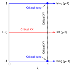
Figure 1: (Color online) Criticality of the transverse-field $XY$ model in the $(\lambda,\gamma)$ parameter space. The transverse-field Ising model $(\gamma=\pm 1)$ has a QCP at $\lambda_{c}=1$. The line $\lambda=1$ represents criticality of the $XY$ model with universality class the same as that of the transverse-field Ising model. The $\gamma=0$ line ($XX$ model) represents the anisotropy transition line for $\lambda\in[0,1]$ with the transition belonging to a new universality class.

The transverse-field $XY$ model and its special case, the transverse-field Ising model (TIM), are well-known statistical mechanical models which illustrate QPTs. A QPT occurs at $T=0$ and is brought about by tuning a non-thermal parameter, e.g., exchange interaction strength, external magnetic field etc. In recent years, quantum information-related measures like entanglement osborne ; osterloh ; amico ; lewenstein , discord sarandy ; werlang and fidelity zanardi have been used as indicators of QPTs. A first-order QPT is characterized by a discontinuity in the first derivative of the ground state energy with respect to the tuning parameter. Similarly in a second-order QPT, termed a critical point QPT, the second derivative of the ground state energy becomes discontinuous or divergent at the critical point. Entanglement and quantum discord (QD) provide different measures of quantum correlations in the mixed state of an interacting many-body system. The QD has so far been defined in the case of a bipartite quantum system. At a first-order QPT point, appropriate entanglement measures and the QD are known to become discontinuous bose ; wu whereas a critical-point QPT is signaled by the discontinuity or divergence of the first derivative of the quantum correlation measures with respect to the tuning parameter wu . The correlations between the different constituents of an interacting quantum system have two distinct components: classical and quantum. While entanglement provides the most well-known example of quantum correlations, the QD captures quantum correlations which are more general than those measured by entanglement ollivier ; henderson . In fact, there are separable mixed states which by definition are unentangled but have non-zero QD.

Quantum systems, in general, are open systems because of the inevitable interaction of a system with its environment. This results in decoherence accompanied by a decay of the quantum correlations in composite systems. A number of recent studies maziero ; almeida ; boas ; vedral ; mazzola ; pal_clust ; pal_ising explore the dynamics of entanglement and QD when the system-environment interactions are taken into account. An interesting result yielded by such studies is that the QD is more robust than entanglement in the case of Markovian (memoryless) dynamics. The QD decays in time vanishing only asymptotically boas ; mazzola ; pal_clust ; pal_ising ; ferraro whereas entanglement undergoes a ‘sudden death’maziero ; almeida , i.e., a complete disappearance at a finite time. The classical correlations, $C\left(\rho_{AB}\right)$, and the QD, $Q\left(\rho_{AB}\right)$, have mostly been computed only for two-qubit systems described by the density matrix $\rho_{AB}$ with $A$ and $B$ denoting the subsystems. Three general types of Markovian time evolution have been observed vedral : (i) $C\left(\rho_{AB}\right)$ is constant as a function of time and $Q\left(\rho_{AB}\right)$ decays monotonically, (ii) $C\left(\rho_{AB}\right)$ decays monotonically over time till a parametrized time $p_{sc}$ is reached and remains constant thereafter. $Q\left(\rho_{AB}\right)$ has an abrupt change in the decay rate at $p_{sc}$, and has magnitude greater than that of $C\left(\rho_{AB}\right)$ in a parametrized time interval, and (iii) both $C\left(\rho_{AB}\right)$ and $Q\left(\rho_{AB}\right)$ decay monotonically. Mazzola et al. mazzola have obtained a significant result that under Markovian dynamics and for a class of initial states the QD remains constant in a finite time interval $0<t<\tilde{t}$. In this time interval, the classical correlations $C\left(\rho_{AB}\right)$ decay monotonically. Beyond $t=\tilde{t}$, $C\left(\rho_{AB}\right)$ becomes constant whereas the QD decreases monotonically as a function of time. The sudden changes in the decay rates of correlations and their constancy in certain time intervals have been demonstrated in actual experiments xu ; auccaise .

In this paper, we consider a two-qubit system each qubit of which interact with an independent reservoir. The density matrix of the two-qubit system is described by the reduced density matrix derived from the ground state of the transverse-field $XY$ model in 1d. A similar study has earlier been carried out for the TIM in 1d pal_ising . We investigate the dynamics of the QD as well as the classical correlations under Markovian time evolution and identify new features close to the quantum critical points of the model. The study is further extended to the cases of further-neighbour two-qubit states and finite temperatures. In Sec. II, the calculational scheme for computing $C\left(\rho_{AB}\right)$ and $Q\left(\rho_{AB}\right)$ is described. We further discuss the methodology for studying the dynamics of the classical and quantum correlations for different quantum channels representing the system-environment interactions. Sec. III presents the major results obtained and the discussions thereof. Sec. IV contains some concluding remarks.

II Classical and quantum correlations: Definition and dynamics

In classical information theory, the total correlation between two random variables $A$ and $B$ is quantified by their mutual information $I(A,B)=H(A)+H(B)-H(A,B)$. The random variables $A$ and $B$ take on the values ‘$a$’  and ‘$b$’  respectively with probabilities given by the sets $\left\{p_{a}\right\}$ and $\left\{p_{b}\right\}$. $H(A)=-\sum_{a}p_{a}\log_{2}p_{a}$ and $H(B)=-\sum_{b}p_{b}\log_{2}p_{b}$ are the Shannon entropies for the variables $A$ and $B$. $H(A,B)=-\sum_{a,b}p_{a,b}\log_{2}p_{a,b}$ is the joint Shannon entropy for the variables $A$ and $B$ with $p_{a,b}$ being the joint probability that the variables $A$ and $B$ have the respective values $a$ and $b$. Generalization to the quantum case is straightforward with the density matrix $\rho$ replacing the classical probability distribution and the von Neumann entropy $S(\rho)=-\mbox{Tr}\left(\rho\log_{2}\rho\right)$ replacing the Shannon entropy. The expression for the quantum mutual information is given by

$$I\left(\rho_{AB}\right)=S\left(\rho_{A}\right)+S\left(\rho_{B}\right)-S\left(\rho_{AB}\right)$$ (2)

An equivalent expression for the classical mutual information is $J(A,B)=H(A)-H(A|B)$ where the conditional entropy $H(A|B)$ is a measure of our ignorance about the state of $A$ when that of $B$ is known. The equivalence with the earlier expression for the classical mutual information can be shown via the Bayes’ rule. The quantum versions of $J(A,B)$ and $I(A,B)$ are not, however, equivalent because the magnitude of the quantum conditional entropy is determined by the type of measurement performed on the subsystem $B$ to gain knowledge of its state. Different measurement choices yield different values for the conditional entropy. We consider von Neumann-type measurements on $B$ represented by a complete set of orthogonal projectors, $\left\{\Pi_{k}^{B}\right\}$, corresponding to the set of possible outcomes $k$. The final state of the composite quantum system after measurement on $B$ is given by $\rho_{k}=\left(I\otimes\Pi_{k}^{B}\right)\rho_{AB}\left(I\otimes\Pi_{k}^{B}\right)/p_{k}$ with $p_{k}=\mbox{Tr}\left(\left(I\otimes\Pi_{k}^{B}\right)\rho_{AB}\left(I\otimes\Pi_{k}^{B}\right)\right)$. $I$ denotes the identity operator for the subsystem $A$ and $p_{k}$ is the probability for obtaining the outcome $k$. The quantum conditional entropy is given by

$$S\left(\rho_{AB}\left|\left\{\Pi_{k}^{B}\right\}\right.\right)=\sum_{k}p_{k}S\left(\rho_{k}\right)$$ (3)

leading to the following quantum extension of the classical mutual information

$$J\left(\rho_{AB},\left\{\Pi_{k}^{B}\right\}\right)=S\left(\rho_{A}\right)-S\left(\rho_{AB}\left|\left\{\Pi_{k}^{B}\right\}\right.\right)$$ (4)

The projective measurements on the subsystem $B$ removes all the non-classical correlations between the subsystems $A$ and $B$. Henderson and Vedral henderson have quantified the total classical correlations $C\left(\rho_{AB}\right)$ by maximizing $J\left(\rho_{AB},\left\{\Pi_{k}^{B}\right\}\right)$ w.r.t. $\left\{\Pi_{k}^{B}\right\}$, i.e.,

$$C\left(\rho_{AB}\right)=\underset{\left\{\Pi_{k}^{B}\right\}}{\max}\left(J\left(\rho_{AB},\left\{\Pi_{k}^{B}\right\}\right)\right)$$ (5)

The difference between the total correlations $I\left(\rho_{AB}\right)$ (Eq. (2)) and the classical correlations $C\left(\rho_{AB}\right)$ (Eq. (5)) defines the QD, $Q\left(\rho_{AB}\right)$,

$$Q\left(\rho_{AB}\right)=I\left(\rho_{AB}\right)-C\left(\rho_{AB}\right)$$ (6)

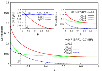
Figure 2: (Color online) Bit-phase-flip channel: Decay of mutual information $I\left(\rho_{AB}\right)$ (solid line), classical correlations $C\left(\rho_{AB}\right)$ (dashed line) and the QD $Q\left(\rho_{AB}\right)$ (dot-dashed line) as a function of the parametrized time $p=1-e^{-\theta t}$ for $\lambda=0.7,\gamma=0.7$. Also, $p_{sc}=0.114$. (inset) (i)The variations of $\left|c_{1}(p)\right|$ (solid line) and $\left|c_{2}(p)\right|$ (dashed line) as functions of $p$. The crossing of $\left|c_{1}(p)\right|$ with $\left|c_{2}(p)\right|$ sets the parametrized time point $p_{sc}$. (ii)Decay of mutual information $I\left(\rho_{AB}\right)$ (solid line), classical correlations $C\left(\rho_{AB}\right)$ (dashed line) and quantum discord $Q\left(\rho_{AB}\right)$ (dot-dashed line) as a function of the parametrized time $p=1-e^{-\theta t}$ for $\lambda=0.7,\gamma=-0.7$.

Though the concept of the QD is well-established, its computation is restricted to mostly two-qubit states. For the two-qubit $X$ states, analytic expressions for the QD can be derived when the density matrix, defined in the computational basis $\left\{|11\rangle,|10\rangle,|01\rangle,|00\rangle\right\}$, has the following structure

$$\rho_{AB}=\left(\begin{array}[]{cccc}a&0&0&f\\ 0&b&z&0\\ 0&z&b&0\\ f&0&0&d\end{array}\right)$$ (11)

where $A$ and $B$ correspond to the two individual qubits and $z$ and $f$ are real numbers. The eigenvalues of $\rho_{AB}$ are sarandy

$$\lambda_{0} = \frac{1}{4}\left\{\left(1+c_{3}\right)+\sqrt{4c_{4}^{2}+\left(c_{1}-c_{2}\right)^{2}}\right\}$$

$$\lambda_{1} = \frac{1}{4}\left\{\left(1+c_{3}\right)-\sqrt{4c_{4}^{2}+\left(c_{1}-c_{2}\right)^{2}}\right\}$$

$$\lambda_{2} = \frac{1}{4}\left(1-c_{3}+c_{1}+c_{2}\right)$$

$$\lambda_{3} = \frac{1}{4}\left(1-c_{3}-c_{1}-c_{2}\right)$$ (12)

with

$$c_{1} = 2z+2f$$

$$c_{2} = 2z-2f$$

$$c_{3} = a+d-2b$$

$$c_{4} = a-d$$ (13)

The mutual information $I\left(\rho_{AB}\right)$ can be written as sarandy

$$I\left(\rho_{AB}\right)=S\left(\rho_{A}\right)+S\left(\rho_{B}\right)+\sum_{\alpha=0}^{3}\lambda_{\alpha}\log_{2}\lambda_{\alpha}$$ (14)

where

$$S\left(\rho_{A}\right)=S\left(\rho_{B}\right) = -\frac{1+c_{4}}{2}\log_{2}\frac{1+c_{4}}{2}$$ (15)

$$-\frac{1-c_{4}}{2}\log_{2}\frac{1-c_{4}}{2}$$

With expressions for $I\left(\rho_{AB}\right)$ and $C\left(\rho_{AB}\right)$ given in Eqs. (14), (15) and (5), the QD, $Q\left(\rho_{AB}\right)$, (Eq. (6)) can in principle be computed. The difficulty lies in carrying out the maximization procedure needed for the computation of $C\left(\rho_{AB}\right)$. It is possible to do so analytically when $\rho_{AB}$ is of the form given in (11) resulting in the following expressions for the QD fanchini :

$$Q\left(\rho_{AB}\right)=\mbox{min}\left\{Q_{1},Q_{2}\right\}$$ (16)

where

$$Q_{1} = S\left(\rho_{B}\right)-S\left(\rho_{AB}\right)-a\log_{2}\frac{a}{a+b}$$ (17)

$$-b\log_{2}\frac{b}{a+b}-d\log_{2}\frac{d}{d+b}-b\log_{2}\frac{b}{d+b}$$

and

$$Q_{2} = S\left(\rho_{B}\right)-S\left(\rho_{AB}\right)-\Delta_{+}\log_{2}\Delta_{+}$$ (18)

$$-\Delta_{-}\log_{2}\Delta_{-}$$

with $\Delta_{\pm}=\frac{1}{2}\left(1\pm\Gamma\right)$ and $\Gamma^{2}=\left(a-d\right)^{2}+4\left(|z|+|f|\right)^{2}$

For spin Hamiltonians with certain symmetries, the two-spin reduced density matrix $\rho_{ij}$ has a form similar to that given in Eq. (11) (the qubits $A$ and $B$ now represent the spins at sites $i$ and $j$ respectively) where the matrix elements of $\rho_{ij}$ can be written in terms of single-site magnetization and two-site spin correlation functions. In the case of the $XY$ model in a transverse-field, the matrix elements of the two-site reduced density matrix are dutta ; osborne ; dillenschneider

$$a = \frac{1}{4}+\frac{\langle\sigma^{z}\rangle}{2}+\frac{\langle\sigma_{i}^{z}\sigma_{j}^{z}\rangle}{4}$$

$$d = \frac{1}{4}-\frac{\langle\sigma^{z}\rangle}{2}+\frac{\langle\sigma_{i}^{z}\sigma_{j}^{z}\rangle}{4}$$

$$b = \frac{1}{4}\left(1-\langle\sigma_{i}^{z}\sigma_{j}^{z}\rangle\right)$$

$$z = \frac{1}{4}\left(\langle\sigma_{i}^{x}\sigma_{j}^{x}\rangle+\langle\sigma_{i}^{y}\sigma_{j}^{y}\rangle\right)$$

$$f = \frac{1}{4}\left(\langle\sigma_{i}^{x}\sigma_{j}^{x}\rangle-\langle\sigma_{i}^{y}\sigma_{j}^{y}\rangle\right)$$ (19)

The finite temperature single-site magnetization $\langle\sigma^{z}\rangle$ in the case of the transverse-field $XY$ model is given by dutta ; dillenschneider

$$\langle\sigma^{z}\rangle=-\frac{1}{\pi}\int_{0}^{\pi}d\phi\tanh{\left(\frac{\beta\omega_{\phi}}{2}\right)}\frac{\left(1+\lambda\cos{\phi}\right)}{\omega_{\phi}}$$ (20)

where

$$\omega_{\phi}=\sqrt{\left(\gamma\lambda\sin{\phi}\right)^{2}+\left(1+\lambda\cos{\phi}\right)^{2}}$$ (21)

describes the energy spectrum and $\beta=\frac{1}{kT}$ with $k$ being the Boltzman constant and $T$ the absolute temperature. The spin-spin correlation functions are obtained from the determinants of Toeplitz matrices dillenschneider ; mccoy ; pfeuty as

$$\left\langle\sigma_{i}^{x}\sigma_{i+r}^{x}\right\rangle = \left|\begin{array}[]{cccc}G_{-1}&G_{-2}&\cdots&G_{-r}\\ G_{0}&G_{-1}&\cdots&G_{-r+1}\\ \vdots&\vdots&\ddots&\vdots\\ G_{r-2}&G_{r-3}&\cdots&G_{-1}\\ \end{array}\right|$$ (26)

$$\left\langle\sigma_{i}^{y}\sigma_{i+r}^{y}\right\rangle = \left|\begin{array}[]{cccc}G_{1}&G_{0}&\cdots&G_{-r+2}\\ G_{2}&G_{1}&\cdots&G_{-r+3}\\ \vdots&\vdots&\ddots&\vdots\\ G_{r}&G_{r-1}&\cdots&G_{1}\\ \end{array}\right|$$ (31)

$$\left\langle\sigma_{i}^{z}\sigma_{i+r}^{z}\right\rangle = \left\langle\sigma^{z}\right\rangle^{2}-G_{r}G_{-r}$$ (32)

where

$$G_{r} = \frac{1}{\pi}\int_{0}^{\pi}d\phi\tanh{\left(\frac{\beta\omega_{\phi}}{2}\right)}\cos(r\phi)\frac{\left(1+\lambda\cos\phi\right)}{\omega_{\phi}}$$ (33)

$$-\frac{\gamma\lambda}{\pi}\int_{0}^{\pi}d\phi\tanh{\left(\frac{\beta\omega_{\phi}}{2}\right)}\sin(r\phi)\frac{\sin\phi}{\omega_{\phi}}$$

with $r=|i-j|$ being the distance between the two spins at the sites $i$ and $j$ (for the nearest-neighbour (n.n.) case, $r=1$).

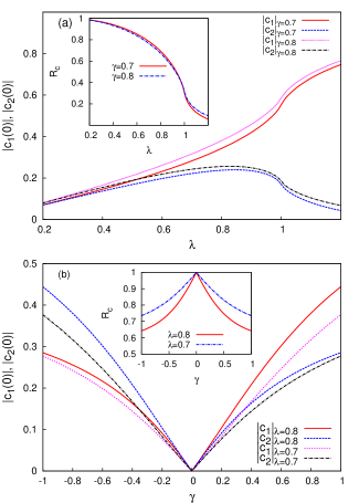
Figure 3: (Color online) (a) Variations of $\left|c_{1}(0)\right|$ and $\left|c_{2}(0)\right|$ with $\lambda$ for $\gamma=0.7$ ($\left|c_{1}(0)\right|$ solid line and $\left|c_{2}(0)\right|$ dashed line) and $\gamma=0.8$ ($\left|c_{1}(0)\right|$ dotted line and $\left|c_{2}(0)\right|$ dot-dashed line). (inset) Variation of $R_{c}$ $\left(=\left|c_{2}(0)\right|/\left|c_{1}(0)\right|\right)$ with $\lambda$ for $\gamma=0.7$ (solid line) and $\gamma=0.8$ (dot-dashed line). (b)Variations of $\left|c_{1}(0)\right|$ and $\left|c_{2}(0)\right|$ with $\gamma$ for $\lambda=0.7$ ($\left|c_{1}(0)\right|$ dotted line and $\left|c_{2}(0)\right|$ dot-dashed line) and $\lambda=0.8$ ($\left|c_{1}(0)\right|$ solid line and $\left|c_{2}(0)\right|$ dashed line). (inset) Variation of $R_{c}$ with $\gamma$ for $\lambda=0.7$ (dot-dashed line) and $\lambda=0.8$ (solid line). $R_{c}=\left|c_{2}(0)\right|/\left|c_{1}(0)\right|$ for $\gamma>0$ (BPF channel) and $R_{c}=\left|c_{1}(0)\right|/\left|c_{2}(0)\right|$ for $\gamma<0$ (BF channel).

We next consider the interaction of the chain of qubits, each qubit representing a $S=\frac{1}{2}$ spin in transverse-field $XY$ model, with an environment. We choose the initial state (time $t=0$) of the whole system at time $t=0$ to be of the product form, i.e.,

$$\rho(0)=\rho_{s}(0)\otimes\rho_{e}(0)$$ (34)

where the density matrices $\rho_{s}$ and $\rho_{e}$ correspond to the system and environment respectively. We assume that the environment is represented by $L$ independent reservoirs each of which interacts locally with a qubit constituting the $XY$ chain. The reduced density matrix obtained from Eq. (34) can be written as

$$\rho_{r}(0)=\rho_{rs}(0)\otimes\rho_{re}(0)$$ (35)

where $\rho_{rs}$ and $\rho_{re}$ represent the two-qubit reduced density matrix of the transverse-field $XY$ chain and the corresponding reduced density matrix of the two-reservoir environment respectively. The quantum channel describing the interaction between a qubit and its environment can be of various types maziero ; nielsenchuang . We first assume the two qubits to represent nearest-neighbour spins in the $XY$ chain. In this paper, we investigate the dynamics of the two-qubit classical and quantum correlations (in the form of the QD) under the influence of the bit-flip (BF), bit-phase-flip (BPF) and phase-flip (PF) channels. In the Kraus operator representation, an initial state, $\rho_{rs}(0)$, of the qubits evolves as boas ; nielsenchuang

$$\rho_{rs}(t)=\sum_{\mu,\nu}E_{\mu,\nu}\rho_{rs}(0)E_{\mu,\nu}^{\dagger}$$ (36)

where the Kraus operators $E_{\mu,\nu}=E_{\mu}\otimes E_{\nu}$ satisfy the completeness relation $\sum_{\mu,\nu}E_{\mu,\nu}E_{\mu,\nu}^{\dagger}=I$ for all $t$. The BF, BPF and PF channels destroy the information contained in the phase relations without involving an exchange of energy. The Kraus operators for these channels are

$$E_{0}=\sqrt{q^{\prime}}\left(\begin{array}[]{cc}1&0\\ 0&1\end{array}\right);\;\;E_{1}=\sqrt{p/2}\sigma_{i}$$ (39)

where $i=x$ for the BF, $i=y$ for the BPF and $i=z$ for the PF channel with $q^{\prime}=1-p/2$. In the case of Markovian time evolution, $p$ is given by $p=1-e^{-\theta t}$ with $\theta$ denoting the decay rate. A fuller description of the channels and the corresponding dynamics can be obtained from Refs. boas ; pal_ising ; nielsenchuang . Using the two-spin reduced density matrix described by Eqs. (11) and (19)-(33) as the initial state $\rho_{rs}(0)$, one can calculate the time-evolved state $\rho_{rs}(t)$ for a specific quantum channel using the Eqs. (36) and (39). Since $\rho_{rs}(t)$ has the same form as Eq. (11), the mutual information, $I(\rho_{AB})$, the QD $Q(\rho_{AB})$ and the classical correlations $C(\rho_{AB})$ can be computed at any time $t$ with the help of the formulae in Eqs. (12)-(18). The main results of our calculations for the various quantum channels are described in the following section.

III Results

III.1 Nearest-neighbour quantum correlations at zero temperature

III.1.1 Bit-flip and bit-phase-flip channels

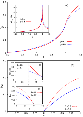
Figure 4: (Color online)(a) Variation of $p_{sc}$ as a function of $\lambda$ with $\gamma=0.7$ (solid line) and $\gamma=0.8$ (dot-dashed line). (inset) The first derivative of $p_{sc}$ w.r.t. $\lambda$ diverges as the QCP $\lambda_{c}=1$ is approached. (b) Variation of $p_{sc}$ as a function of $\gamma$ with $\lambda=0.7$ (solid line) and $\lambda=0.8$ (dot-dashed line) for the BPF channel. (inset) (i) The first derivative of $p_{sc}$ w.r.t. $\gamma$ exists when $\gamma_{c}>0$ for the BPF channel. (ii) Variation of $p_{sc}$ as functions of $\gamma$ with $\lambda=0.7$ (solid line) and $\lambda=0.8$ (dot-dashed line) for the BF channel.

We first consider the case of $T=0$ so that the $XY$ spin chain is in its ground state. In the case of the BPF channel, the dynamical evolutions of the mutual information $I\left(\rho_{AB}\right)$, the classical correlations $C\left(\rho_{AB}\right)$, the QD $Q\left(\rho_{AB}\right)$ and the absolute values of the coefficients $c_{1}$ and $c_{2}$ as a function of the parametrized time $p$ $(p=1-e^{-\theta t})$ are shown in Fig. 2 for $\lambda=\gamma=0.7$. The dynamics are similar to type (ii) where sudden changes in the decay rates of the classical correlations and the QD occur at a parametrized time instant $p_{sc}$. Inset (a) shows the variations of $\left|c_{1}(p)\right|$ and $\left|c_{2}(p)\right|$ versus $p$. The crossing point is given by $p_{sc}$. Inset (b) shows the time-evolutions of the mutual information, the classical correlations and the QD for $\lambda=0.7$, $\gamma=-0.7$ which are described by type (iii) dynamics, i.e., both $C\left(\rho_{AB}\right)$ and $Q\left(\rho_{AB}\right)$ decay monotonically. The dynamics in the case of the BF channel have an interesting correspondence with the dynamics of the BPF channel. Type (ii) and Type (iii) dynamics are obtained in the case of the BPF (BF) channel for +ve (-ve) and -ve (+ve) values of $\gamma$ respectively. The following analysis provides us with an understanding of this result. The rules of evolution for the coefficients $c_{1}$ and $c_{2}$ are obtained from Eqs. (11), (13), (36) and (39) in the cases of the BPF and BF channels. These are given by

BPF Channel:

$$c_{1}(p) = c_{1}(0)(1-p)^{2}$$

$$c_{2}(p) = c_{2}(0)$$

$$c_{3}(p) = c_{3}(0)(1-p)^{2}$$

$$c_{4}(p) = c_{4}(0)(1-p)$$ (40)

BF Channel:

$$c_{1}(p) = c_{1}(0)$$

$$c_{2}(p) = c_{2}(0)(1-p)^{2}$$

$$c_{3}(p) = c_{3}(0)(1-p)^{2}$$

$$c_{4}(p) = c_{4}(0)(1-p)$$ (41)

From Eqs. (13) and (19), the coefficients $c_{1}(0)$ and $c_{2}(0)$ are identified as the two-spin correlation functions $\langle\sigma_{i}^{x}\sigma_{j}^{x}\rangle$ and $\langle\sigma_{i}^{y}\sigma_{j}^{y}\rangle$ respectively (in the present study, $r=|i-j|=1$). Fig. 3(a) shows the variation of the absolute values of the coefficients $c_{1}(0)$ and $c_{2}(0)$ with $\lambda$ for $\gamma>0$. The general observation is that for $\gamma>0$, $\left|c_{1}(0)\right|\geq\left|c_{2}(0)\right|$ for $\lambda\in[0,1]$. Fig. 3(b) shows the plots of $\left|c_{1}(0)\right|$ and $\left|c_{2}(0)\right|$ versus $\gamma$ for fixed $\lambda$ values. One finds that when $\gamma$ is $<0$, $\left|c_{1}(0)\right|\leq\left|c_{2}(0)\right|$ for $\lambda\in[0,1]$. Since $\left|c_{1}(0)\right|\geq\left|c_{2}(0)\right|$ for $\gamma>0$, Eq. (40), describing the rules of evolution for the BPF channel, indicates that in this case there is a certain parametrized time instant at which $\left|c_{1}(p)\right|$ crosses $\left|c_{2}(p)\right|\left(=\left|c_{2}(0)\right|\right)$. This specific value turns out to be the same as $p_{sc}$ at which a sudden change in the decay rates of the classical and quantum correlations occur (Fig. 2). From the condition $\left|c_{1}(p)\right|=\left|c_{2}(p)\right|$ and Eq. (40), one obtains the following expression for $p_{sc}$ in the case of the BPF channel:

$$p_{sc}=1-\sqrt{R_{c}}$$ (42)

where $R_{c}=\left|c_{2}(0)\right|/\left|c_{1}(0)\right|$. The QD (BPF channel, $\gamma>0$) is given by $Q_{2}$ in Eq. (18) for $p\in[0,1]$. At $p=p_{sc}$, $\left(c_{1}(p)-c_{2}(p)\right)$ or $\left(c_{1}(p)+c_{2}(p)\right)$ changes sign depending on whether $c_{1}(0)$ and $c_{2}(0)$ have the same or different signs respectively. Noticing that $z(p)=\left(c_{1}(p)+c_{2}(p)\right)/4$ and $f(p)=\left(c_{1}(p)-c_{2}(p)\right)/4$ (Eq. (13)), the magnitude of $\Gamma$ which involves $|z|$ and $|f|$ (Eq. (18)) changes at the point $p=p_{sc}$, while $S\left(\rho_{B}\right)$ and $S\left(\rho_{AB}\right)$ remain unchanged, thus bringing about the sudden change in the decay rates of the quantum correlations. With $\gamma<0$, $\left|c_{1}(0)\right|$ is $\leq\left|c_{2}(0)\right|$ so that $c_{1}(p)$ never crosses $c_{2}(p)$ and one obtains type (iii) dynamics. We next compare the rules of evolution for the BF channel (Eq. (41)) with those of the BPF channel (Eq. (40)). One finds that the rules of evolution for $c_{3}(p)$ and $c_{4}(p)$ remain identical while those for $c_{1}(p)$ and $c_{2}(p)$ are interchanged. This explains the interchange of dynamics type mentioned earlier: for $\gamma>0$, since $\left|c_{1}(0)\right|$ is $\geq\left|c_{2}(0)\right|$, $c_{1}(p)$ never crosses $c_{2}(p)$ for the BF channel so that type (iii) dynamics hold true whereas for $\gamma<0$, the crossing point is given by $R_{c}=\left|c_{1}(0)\right|/\left|c_{2}(0)\right|$. The effective interchange in the identities of $c_{1}(0)$ and $c_{2}(0)$ across the $\gamma=0$ (critical $XX$) line is understood by remembering that $c_{1}(0)=\langle\sigma_{i}^{x}\sigma_{i+1}^{x}\rangle$ and $c_{2}(0)=\langle\sigma_{i}^{y}\sigma_{i+1}^{y}\rangle$. The correlation function $\langle\sigma_{i}^{x}\sigma_{i+1}^{x}\rangle$ is interchanged with $\langle\sigma_{i}^{y}\sigma_{i+1}^{y}\rangle$ under the transformation $\gamma\rightarrow-\gamma$ (see Eqs. (32) and (33)). The variations of $R_{c}$ with $\lambda$ and $\gamma$ are shown in the insets of Fig. 3.

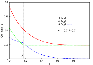
Figure 5: (Color online) Phase-flip channel: Decay of mutual information $I\left(\rho_{AB}\right)$ (solid line), classical correlations $C\left(\rho_{AB}\right)$ (dashed line) and quantum discord $Q\left(\rho_{AB}\right)$ (dot-dashed line) as a function of the parametrized time $p=1-e^{-\theta t}$ for $\lambda=0.7,\gamma=\pm 0.7$. In this case, $p_{sc}=0.173$.

Fig. 4(a) shows the plots of $p_{sc}$ and the first derivative of $p_{sc}$ w.r.t. $\lambda$, $\left(\frac{dp_{sc}}{d\lambda}\right)_{\gamma}$ (inset), as functions of $\lambda$ for the BPF channel $(\gamma>0)$. The first derivative of $p_{sc}$ w.r.t. $\lambda$ diverges as the quantum critical point (QCP) $\lambda_{c}=1$ is approached. Fig. 4(b) shows the variation of $p_{sc}$ with the anisotropy parameter $\gamma$ for the BPF channel. As expected, $p_{sc}\neq 0$ for $\gamma>0$. Both $\left|c_{1}\right|$ and $\left|c_{2}\right|$ individually tend to zero as $\gamma\rightarrow 0$ for $\lambda\in[0,1]$ and the ratio $R_{c}\left(=\left|c_{2}(0)\right|/\left|c_{1}(0)\right|\right)\rightarrow 1$ as $\gamma\rightarrow 0$ (Fig. 3). The inset (i) shows the variation of the first derivative of $p_{sc}$ w.r.t. $\gamma$, $\left(\frac{dp_{sc}}{d\gamma}\right)_{\lambda}$, as a function of $\gamma$ for fixed values of $\lambda$. The first derivative of $p_{sc}$ w.r.t. $\gamma$ shows a discontinuity at the anisotropy transition point, $\gamma=0$, indicating a QPT. Inset (ii) shows the variation of $p_{sc}$ as a function of $\gamma$ for the BF channel ($p_{sc}\neq 0$ for $\gamma<0$). In a recent study pal_ising , we have investigated the Markovian evolution of the classical and quantum correlations for a number of quantum channels in the case of the transverse-field Ising model, a special case ($\gamma=1$) of the transverse-field $XY$ model considered in this paper. For the BPF channel, we have pointed out that the first derivative of the parametrized time instant at which the sudden changes in the decay rates of classical and quantum correlations occur w.r.t. $\lambda$ diverges as the Ising model critical point $\lambda_{c}=1$ is approached. We have further shown that the BPF (BF) channel exhibits only type (ii) (type (iii)) dynamics. In the case of the $XY$ model, positive and negative values of the anisotropy parameter $\gamma$ allow for both type (ii) ($\gamma<0$) and (iii) ($\gamma>0$) dynamics for the BF channel. Similarly, unlike in the case of the transverse-field Ising model, type (iii) dynamics are possible for the BPF channel ($\gamma<0$).

III.1.2 Phase-flip channel

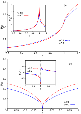
Figure 6: (Color online)(a) Variation of $p_{sc}$ as functions of $\lambda$ with $\gamma=0.7$ (solid line) and $\gamma=0.8$ (dot-dashed line) in the case of the PF channel. (inset) The first derivative of $p_{sc}$ w.r.t. $\lambda$ diverges as the QCP $\lambda_{c}=1$ is approached. (b) Variation of $p_{sc}$ as functions of $\gamma$ with $\lambda=0.7$ (solid line) and $\lambda=0.8$ (dashed line) for the PF channel. (inset) The first derivative of $p_{sc}$ as a function of $\gamma$ becomes discontinuous at the anisotropy transition point $\gamma_{c}=0$.

The variations of the mutual information $I\left(\rho_{AB}\right)$, classical correlations $C\left(\rho_{AB}\right)$ and QD $Q\left(\rho_{AB}\right)$ versus the parametrized time $p$ for $(\lambda=0.7,\gamma=\pm 0.7)$ have been plotted in Fig. 5 in the case of the PF channel. The dynamics is of type (ii) and there is a specific time interval during which the QD is greater in magnitude than that of the classical correlations. The classical correlations remain constant at a value $I\left(\rho_{AB}\right)_{p=1}$, the mutual information of the fully decohered state, in the parametrized time interval $p_{sc}<p<1$. In the interval $0<p<p_{sc}$, the classical correlations decay with time. On the other hand, the quantum correlations, as measured by the QD, undergoes a sudden change in its decay rate at $p=p_{sc}$ and goes to zero in the asymptotic limit $p\rightarrow 1$. One must note that the type of the dynamics in the case of the PF channel is unchanged under a change in sign of the anisotropy parameter $\gamma$, the reason of which can be easily understood by examining the evolution rules for the coefficients $c_{i}$’s from Eq. (11), (13), (36) and (39):

$$c_{1}(p) = c_{1}(0)(1-p)^{2}$$

$$c_{2}(p) = c_{2}(0)(1-p)^{2}$$

$$c_{3}(p) = c_{3}(0)$$

$$c_{4}(p) = c_{4}(0)$$ (43)

Both the coefficients $c_{1}$ and $c_{2}$ decay with time identically in the case of the PF channel whereas the other coefficients remain independent of time. Since the change in sign of the anisotropy parameter $\gamma$ only interchanges the values of $c_{1}$ and $c_{2}$, it can not affect the dynamics that the classical and quantum correlations undergo in the PF channel. In this case, the sudden change in the decay rates of $Q\left(\rho_{AB}\right)$ and $C\left(\rho_{AB}\right)$ at $p=p_{sc}$ is understood by noting that in the interval $0<p<p_{sc}$, the QD is determined by $Q\left(\rho_{AB}\right)=Q_{2}$ (Eq. (18)) and for $p_{sc}<p<1$, $Q\left(\rho_{AB}\right)=Q_{1}$ (Eq. (17)). In the regime $p_{sc}<p<1$, $C\left(\rho_{AB}\right)$ is given by

$$C\left(\rho_{AB}\right) = S\left(\rho_{A}\right)+a\log_{2}\frac{a}{a+b}+b\log_{2}\frac{b}{a+b}$$ (44)

$$+d\log_{2}\frac{d}{d+b}+b\log_{2}\frac{b}{d+b}$$

The matrix elements $a$, $b$ and $d$ are functions of only $c_{3}$ and $c_{4}$ which are independent of time (Eq. (43)). From Eq. (15), $S\left(\rho_{A}\right)$, being a function of $c_{4}$ only, is also independent of $p$, thereby ensuring the constancy of the classical correlations $C\left(\rho_{AB}\right)$. The time instant $p_{sc}$ can be determined as a solution of the equation $Q_{1}=Q_{2}$. Fig. 6(a) shows the variation of $p_{sc}$ as a function of the inverse of the strength of the transverse field, $\lambda$. The first derivative of $p_{sc}$ w.r.t. $\lambda$ for a fixed value of the anisotropy parameter $\gamma$ diverges as the QPT point $\lambda_{c}=1$ is approached (although the results for positive $\gamma$ values only have been shown, identical result can be obtained for negative $\gamma$ values as well). Fig. 6(b) demonstrates the variation of $p_{sc}$ versus $\gamma$ for fixed $\lambda$ values. The behaviour of $p_{sc}$ is symmetric across the anisotropy transition point $\gamma=0$. On approaching $\gamma=0$, $p_{sc}$ goes to zero. The inset of Fig. 6(b) shows the variation of the first derivative of $p_{sc}$ w.r.t. $\gamma$ at the QCP $\gamma=0$. The landscapes of $p_{sc}$ versus the inverse of the transverse-field strength $\lambda$ and the anisotropy parameter $\gamma$ are shown in Fig. 7.

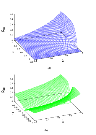
Figure 7: (Color online) (a) Variation of $p_{sc}$ as a function of the system parameters $\lambda$ and $\gamma$ for the BPF channel (b) Variation of $p_{sc}$ as a function of the system parameters $\lambda$ and $\gamma$ for the PF channel.

III.2 Further-neighbour quantum correlations at zero temperature

We have so far considered the spins in a pair to be n.n.s. The dynamics of the QD when the spins are separated by further neighbour distances can be investigated following the procedure outlined in Sec. II. The two qubit reduced density matrix $\rho_{sc}(0)$ (Eq. (36)) now involves further-neighbour spin-spin correlation functions (Eqs. (32) and (33) with $r>1$). Fig. 8 shows the decay of the mutual information $I\left(\rho_{AB}\right)$ (solid line), the classical correlations $C\left(\rho_{AB}\right)$ (dashed line) and the QD $Q\left(\rho_{AB}\right)$ (dot-dashed line) as a function of the parametrized time $p=1-e^{-\theta t}$ for $\lambda=0.7,\;\gamma=0.7$ in the cases of the BPF ($r=2$ (a) and $r=3$ (b)) and the PF ($r=2$ (c) and $r=3$ (d)) channels with $r=2$ and $3$ corresponding respectively to second and third neighbour distances between the spins in a pair. Comparing Fig. 8 with Figs. 2 and 5 one finds that the magnitude of $p_{sc}$ in the case of the PF channel is larger than that in the case of the BPF channel. Our computation shows that this feature is obtained when $r=1$ irrespective of whether $\lambda$ is less or greater than the QCP $\lambda_{c}=1$. For $r>1$, however, the magnitude of $p_{sc}$ in the case of the BPF channel is less than that in the case of the PF channel only for $\lambda<\lambda_{c}$. At $\lambda>\lambda_{c}$, the reverse trend is observed. Also, for the same type of channel, BPF or PF, the magnitude of $p_{sc}$ shifts towards larger values as $r$, the separation between the two qubits (spins) increases. Fig. 9 shows the divergence of $\frac{dp_{sc}}{d\lambda}$ at the QCP $\lambda_{c}=1$ for $r=2$ and $3$ and the BPF (a) and the PF(b) channels with $\gamma=0.7$. Maziero et. al. mazieroxy ; mazieroxy2 have shown that in the case of the transverse-field $XY$ chain, the QD for spin-pairs with $r>1$ is able to signal a QPT whereas pairwise entanglement is non-existent for such distances. They have further demonstrated a noticeable change in the decay rate of the QD as a function of $r$ as the system crosses the critical point $\lambda=1$. The decay rate is slower for $\lambda>1$, i.e., in the ferromagnetic phase. In the presence of system-environment interactions, the QD evolves as a function of time. We select three time points (three different $p$ values) at which we compute the QD for $r=1,2,3$ and $4$. Figs. 10 (a) and (c) show the results for the BPF and PF channels respectively for $\gamma=0.7$ and $\lambda=0.7$, i.e., $\lambda<\lambda_{c}=1$. Figs. 10 (b) and (d) show the corresponding plots when $\lambda$ is $>\lambda_{c}$ with $\lambda=1.1$. We find that the decay of the QD as a function of $r$ becomes considerably slower as the QCP $\lambda_{c}=1$ is crossed in the case of both the BPF and PF channels.

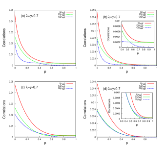
Figure 8: (Color online) Decay of the mutual information $I\left(\rho_{AB}\right)$ (solid line), the classical correlations $C\left(\rho_{AB}\right)$ (dashed line) and the QD $Q\left(\rho_{AB}\right)$ (dot-dashed line) as a function of the parametrized time $p=1-e^{-\theta t}$ for $\lambda=0.7,\;\gamma=0.7$ in the cases of the BPF ($r=2$ (a) and $r=3$ (b)) and the PF ($r=2$ (c) and $r=3$ (d)) channels. Insets of (b) and (d) show on a magnified scale the sudden changes in the decay rates of the correlations

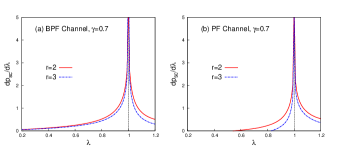
Figure 9: (Color online) The divergence of $\frac{dp_{sc}}{d\lambda}$ at the QCP $\lambda_{c}=1$ in the cases of $r=2$ and $r=3$ and for the BPF (a) and PF (b) channels with the anisotropy parameter $\gamma=0.7$

III.3 Quantum correlations at finite temperatures

The dynamics of the QD at finite temperatures ($T\neq 0$) and for different values of $r$ are investigated using the procedure described in Sec. II. For infinite chain spin models like the $XXZ$ chain (in the presence and absence of magnetic field) and the transverse-field $XY$ chain, the thermal quantum discord (TQD) has been shown to detect the critical points of QPTs at finite temperatures werlang ; werlang2 ; werlang3 . In fact, the TQD is a better indicator of QPTs than thermodynamic quantities and different entanglement measures. Fig. 11 displays our results when system-environment interactions, which give rise to the dynamics of quantum correlations, are taken into account. The first (second) column in the figure pertains to the BPF (PF) channel. The finite temperature calculations are carried out for different two-qubit distances, e.g., $r=1,2$ and $3$. An examination of Fig. 11 shows that at finite temperature, the first derivative $\frac{dp_{sc}}{d\lambda}$ no longer diverges at the QCP $\lambda_{c}=1$ but exhibits a maximum which is shifted from the QCP. With increasing $T$ and $r$, the shift is greater in magnitude and the maximum becomes more broadened. The last row of Fig. 11 shows the estimated QCP at $T\neq 0$ and for $r=1,2,3$, given by the $\lambda$ value at which the maximum of the $\frac{dp_{sc}}{d\lambda}$ versus $\lambda$ plot occurs. In the case of the BPF channel, the estimated QCP is always lower than $\lambda_{c}=1$ for all values of $r$ whereas in the case of the PF channel, the estimated QCP lies above the $\lambda_{c}=1$ value for $r\geq 2$.

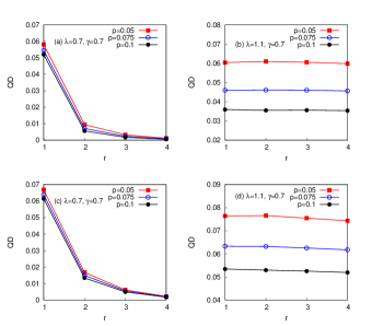
Figure 10: (Color online) Decay of the QD as a function of $r$ at three parametrized time points $\left(p=1-e^{-\theta t}\right)$ for the (a),(b) BPF and (c),(d) PF channels. For each channel, the decay slows down considerably as the QCP $\lambda_{c}=1$ is crossed. The $p$ values considered are $p=0.05$ (solid squares), $p=0.075$ (empty circle) and $p=0.1$ (solid circle). Also $\lambda=0.7$ ((a),(c)), $1.1$ ((b),(d)) and $\gamma=0.7$

IV Concluding remarks

The transverse-field $XY$ model in 1d and its derivative model, the transverse-field Ising model, are well-known spin models which exhibit QPTs. The models have been extensively studied in recent years from the perspective of quantum information theory to quantify the different types of quantum correlations like bipartite/multipartite entanglement and quantum discord (QD), present in the ground and thermal states of the system, as a function of different model parameters. One significant fact which emerges from these studies is that the quantum correlation measures can provide signatures of QPTs. Another interesting line of study involves probing the dynamics of different type of correlations, both classical and quantum, due to the inevitable interaction of a quantum system with its environment resulting in decoherence. In this paper, we study the Markovian time evolution of two-qubit states in the Kraus operator formalism due to the local interactions of the qubits with independent environments. The two-qubit state is described by the nearest-neighbour reduced density matrix of the transverse-field $XY$ model ground state in 1d. The quantum channels, representing system-environment interactions, are of three types: bit-flip, bit-phase-flip and phase-flip. We investigate the dynamics of the mutual information $I\left(\rho_{AB}\right)$, a measure of the total correlations in the system, the classical correlations $C\left(\rho_{AB}\right)$ and the QD, $Q\left(\rho_{AB}\right)$ as a function of the parametrized time $p$. An earlier study vedral identified three different types of dynamics for a different set of initial states of which only the type (ii) and (iii) dynamics are observed in the present study. A significant result of our study is to identify quantities, $\frac{dp_{sc}}{d\lambda}$ and $\frac{dp_{sc}}{d\gamma}$, associated with the type (ii) dynamics which diverges and becomes discontinuous, respectively, as a quantum critical point is approached. The discontinuity occurs as the critical point $\gamma=0\;(\lambda\in[0,1])$ of the anisotropy transition is approached and the divergence is obtained as the quantum critical point $\lambda=1$ is approached.

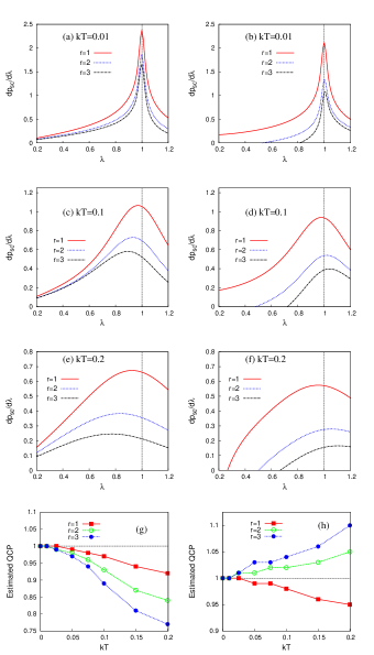
Figure 11: (Color online) The variation of $\frac{dp_{sc}}{d\lambda}$ versus $\lambda$ for $r=1$ (solid line), $r=2$ (dotted line) and $r=3$ (dashed line) at temperatures $kT=0.01,0.1$ and $0.2$. The first (second) column refers to the BPF (PF) channel. In (g) and (h) the estimated QCPs are plotted against $kT$ for the BPF (g) and PF (h) channels respectively and for $r=1$ (solid squares), $r=2$ (empty circles) and $r=3$ (solid circles) with $\gamma=1$.

The two different types of critical point transitions belong to two different universality classes. We find an interesting correspondence between the dynamics of bit-flip and bit-phase-flip channels, namely, the dynamics type is interchanged across the $\gamma=0$ line. We provide an explanation for this feature and obtain an analytic expression for $p_{sc}$, the parametrized time point at which a sudden change in the decay rates of the classical and quantum correlations occur. The transverse-field $XY$ model has a phase diagram richer than that of the transverse-field Ising model. This is reflected in the varied dynamics possible for a single quantum channel in the first case. The BPF and BF channels in the case of the transverse-field Ising model are characterized by their specific type of dynamics pal_ising whereas in the case of the $XY$ model, the dynamics type changes across the $\gamma=0$ line. We have further extended our study to finite temperatures and to $r$ (the distance of separation between the two qubits described by the reduced density matrix) beyond the n.n. distance. In the latter case for $T=0$, one finds that the derivatives $\frac{dp_{sc}}{d\lambda}$ diverges at the QCP $\lambda_{c}=1$ as in the case of $r=1$. We have further demonstrated that at a specific time point, the decay of the QD as a function of $r$ becomes significantly slower as the QCP $\lambda_{c}=1$ is crossed. We have obtained the results for the BPF and the PF channels but the same feature holds true for other channels like the amplitude damping channel. We have checked that the decay rate decreases continuously as the QCP is approached. At finite temperatures, the TQD is able to provide estimates of critical points associated with QPTs, this is true for both n.n. as well as further-neighbour qubits though higher temperatures and larger values of $r$ smear out the signatures. The general trends obtained are similar to those derived in the case of isolated systems, i.e., when system-environment interactions are ignored. In all our computations, we have not, however, obtained any evidence of the type (i) dynamics mentioned in Sec. I. In the present study, we have considered the time evolution of the quantum correlations to be Markovian in nature, an issue of significant interest would be to look for signatures of QPTs in the case of non-Markovian time evolution.

References

- (1) E. Lieb, T. Schultz and D. Mattis, Ann. Phys. 60, 407 (1961)
- (2) E. Barouch and B. McCoy, Phys. Rev. A 3, 786 (1971)
- (3) P. Pfeuty, Ann. Phys. 57, 79 (1970)
- (4) M. Zhong and P. Tong, J. Phys. A: Math. Theor. 43, 505302 (2010)
- (5) A. Dutta, U. Divakaran, B. K. Chakrabarti, T. F. Rosenbaum and G. Aeppli, arXiv:1012.0653v1 [cond-mat.stat-mech]
- (6) J. Osborne and M. A. Nielsen, Phys. Rev. A 66, 032110 (2002)
- (7) A. Osterloh, L. Amico, G. Falci and R. Fazio, Nature 416, 608 (2002)
- (8) L. Amico, R. Fazio, A. Osterloh and V. Vedral, Rev. Mod. Phys. 80, 517 (2008)
- (9) M. Lewenstein, A. Sanpera, V. Ahufinger, B. Damski, A. Sen and U. Sen, Adv. Phys. 56, 243 (2007)
- (10) M. S. Sarandy, Phys. Rev. A 80, 022108 (2009)
- (11) R. Dillenschneider, Phys. Rev. B 78, 224413 (2008)
- (12) T. Werlang, G. A. P. Ribeiro and G. Rigolin, Phys. Rev. A 83, 062334 (2011)
- (13) P. Zanardi and N. Paunković, Phys. Rev. E 74, 031123 (2006)
- (14) I. Bose and E. Chattopadhyay, Phys. Rev. A 66, 062320 (2002)
- (15) L. -A. Wu. M. S. Sarandy and D. A. Lidar, Phys. Rev. Lett. 93, 250403 (2004)
- (16) H. Ollivier and W. H. Zurek, Phys. Rev. Lett. 88, 017901 (2001)
- (17) L. Henderson and V. Vedral, J. Phys. A: Math. Gen. 34, 6899 (2001)
- (18) J. Maziero, T. Werlang, F. F. Fanchini, L. C. Céleri and R. M. Serra, Phys. Rev. A 81, 022116 (2010)
- (19) M. P. Almeida et al., Science 316, 579 (2007)
- (20) T. Werlang, S. Souza, F. F. Fanchini and C. Villas Boas, Phys. Rev. A 80, 024103 (2009)
- (21) J. Maziero, L. C. Céleri, R. M. Serra and V. Vedral, Phys. Rev. A 80, 044102 (2009)
- (22) L. Mazzola, J. Piilo and S. Maniscalco, Phys. Rev. Lett. 104, 200401 (2001)
- (23) A. K. Pal and I. Bose, J. Phys. B: At. Mol. Opt. Phys. 44, 045101 (2011)
- (24) A. K. Pal and I. Bose, Eur. Phys. J. B 85:36 (2012)
- (25) A. Ferraro, L. Aolita, D. Cavalcanti, F. M. Cucchietti and A. Acin, Phys. Rev. A 81, 052318 (2010)
- (26) J. -S. Xu, X. -Y. Xu, C. -F. Li, C. -J. Zhong, X. -B. Zoa and G. -C. Guo, Nat. Commun. 1, 7 (2010)
- (27) R. Auccaise et al., Phys. Rev. Lett. 107, 140403 (2011)
- (28) F. F. Fanchini, T. Werlang, C. A. Brasil, L. G. E. Arruda and A. O. Caldeira, Phys. Rev. A 81 052107 (2010)
- (29) M. A. Nielsen and I. L. Chuang, Quantum Computation and Quantum Information (Cambridge University Press, Cambridge, England, 2000)
- (30) J. Maziero, H. C. Guzman, L. C. Céleri, M. S. Sarandy and R. M. Serra, Phys. Rev. A 82, 012106 (2010)
- (31) J. Maziero, L. C. Céleri, R. M. Serra and M. S. Sarandy, Phys. Lett. A 376, 1540 (2012)
- (32) T. Werlang, C. Trippe, G. A. P. Ribeiro and G. Rigolin, Phys. Rev. Lett. 105, 095702 (2010)
- (33) T. Werlang, G. A. P. Ribeiro and G. Rigolin, Int. J. Mod. Phys. B 27, 1345032 (2013)