Google in a Quantum Network

Abstract

We introduce the characterization of a class of quantum PageRank algorithms in a scenario in which some kind of quantum network is realizable out of the current classical internet web, but no quantum computer is yet available. This class represents a quantization of the PageRank protocol currently employed to list web pages according to their importance. We have found an instance of this class of quantum protocols that outperforms its classical counterpart and may break the classical hierarchy of web pages depending on the topology of the web.

I Introduction

The possibility of establishing a quantum network of practical use is currently under active investigation. Some early versions of them, modest as they may be, have been designed and realized in real world in the recent years darpa ; SECOQC ; UQCC ; SwissQuantum ; vicente1 ; ETSI , or in some instances they are under way. In fact, building a quantum network has been targeted as a fundamental goal in quantum information NC ; rmp an even a more feasible goal to accomplish than the first scalable quantum computer. There are other more advanced proposals for quantum networks quantum_internet1 ; quantum_internet2 based on entanglement connections that need quantum repeaters qrepeaters98 ; qrepeaters99 ; rmprepaters in order to function properly and being stable telecomunications11 ; qap10 ; telecomunications10 . Related to this, some physical quantum models exhibit very remarkable long-distance entanglement properties mps03 ; le04 ; korepin ; graph_states . Another alternative to build different types of quantum networks makes use of quantum percolation protocols percolation07 ; distribution10 ; calsamiglia09 ; calsamiglia11 .

Thus, it is interesting to study how different possibilities of quantum networks would behave regarding what we know about the world wide web. In particular, an essential ingredient in the classical network that we enjoy today is the ability to search web pages in the immense changing world that the web has come to be known. The key tool for performing those searches is the notion of the PageRank algorithm BrinPage98 ; BrinPage98a ; BrinPage98b ; LangvilleMeyer04 ; Meyer00 ; HaveliwalaKamvar03 ; marijuan11 ; shepelyansky ; vitanyi .

We envision a similar tool to perform the task of ranking quantum webpages. A quantum webpage is a node of the quantum network realized by means of a quantum storage device, like a quantum memory. What is crucially important is that a fully fledged quantum computer is not required. Thus, the quantum webpages have limited capabilities: storing and reading in/out quantum states.

Since the notion of a quantum PageRank is by no means unique, it is convenient to introduce a class or category of possible quantum PageRanks. They must satisfy a set of properties that define an admissible class:

Quantum Computer PageRank Class:

Q1

The classical PageRank must be embedded into the quantum class in such a way that the directed graph structure is preserved at the quantum level.

Q2

The sum of all quantum PageRanks must add to 1 i.e. $\sum_{i}I_{q}(P_{i})=1$.

Q3

The Q-PageRank admits a quantized Markov Chain (MC) description.

Q4

The classical algorithm to compute the quantum computer PageRank belongs to the computational complexity class BQP.

However, as we have noticed that working with a real quantum computer seems not realistic in the near future and prospects for realizing quantum networks based on nodes made up of quantum storing devices, like quantum memories, are high as shown by experimental progress, we find also very convenient to introduce a more realistic class of quantum PageRanks as follows:

Quantum PageRank Class:

P1

The classical PageRank must be embedded into the quantum class in such a way that the directed graph structure is preserved at the quantum level.

P2

The sum of all quantum PageRanks must add to 1 i.e. $\sum_{i}I_{q}(P_{i})=1$.

P3

The Q-PageRank admits a quantized Markov Chain (MC) description.

P4

The classical algorithm to compute the quantum PageRank belongs to the computational complexity class P.

The crucial difference is the substitution of property Q4 that deals with the feasibility of calculations with a quantum computer in polynomial time by property P4 which is more demanding since it means that even a classical computer can simulate the process and find the importance of webpages in polynomial time.

Property P1 reflects the fact that originally we would have an internet that is a classical network represented by a directed graph and then shall apply some kind of quantization procedure in order to turn it into a quantum network. The latter must be compatible with the classical one, particularly preserving the directed structure which is crucial to measure a page’s authority. This is non-trivial and some quantization methods may fail to produce a unitary quantum PageRank importance for the quantum case, as shown in Sect.III.

With property P2 we guarantee that we have a globally well-defined notion of the importance of a web page at the quantum level. This allows us to have the probabilistic interpretation of the surfer’s position (see Sect.III).

Property P3 is the key to a wide class of natural quantization methods for the classical PageRank based in the equivalence of this one with a classical Markov chain process (see Sect.III). Thus, it is natural that the equivalent property holds true in the quantum version of the PageRank, and consequently, its description in terms of a quantized surfer’s motion.

The reason for property P4 relies on the assumption that we envisage a near-future scenario when a certain class of quantum network will be operative but not yet a scalable quantum computer. Therefore, we demand that the computation of the quantum PageRank $I_{q}$ be efficiently carried out on a classical computer.

In this paper we have constructed a valid quantum PageRank that fulfills all these requirements. We remark that there may be other solutions to the quantum version of the PageRank within the class defined above, but nevertheless we shall show that finding one instance of this quantum PageRank class is a non-trivial task.

The definition of Class of Quantum PageRank given here is very general and it can accommodate very diverse situations, ranging from quantum channels (including entangled states) between nodes in the network to simpler situations where network nodes are quantum levels of a multilevel quantum system where information is stored in the same way as in the Grover algorithm. In the particular instance of Quantum PageRank algorithm that we have found in subsection Results: A Quantization of Google PageRank , we are concerned with the latter case of a multilevel quantum systems where the quantum state is attached to a link of the network of nodes. This instance does not exhaust all possibilities represented in our generic Class of Quantum PageRanks by all means, but it is the first non-trivial instance in which sharp deviations from the classical PageRank algorithm can be found, as explained later on in our paper.

The explicit step-by-step description of our quantum PageRank algorithm is presented in Sect.IV. A key distinctive feature of this quantum algorithm is that the importance of the quantum pages exhibit quantum fluctuations unlike its classical counterpart. These quantum fluctuations, as shown in the simulations in Sect.V, show up in the form of time dependent importances $I_{q}(P_{i},t)$, which causes in turn that sometimes one certain pair of pages satisfy $I_{q}(P_{i},t_{1})>I_{q}(P_{j},t_{1})$, and some other times the relative importance is reversed $I_{q}(P_{i},t_{2})<I_{q}(P_{j},t_{2})$, for time-steps such that $t_{1}<t_{2}$. We may use an analogy to understand this situation: the classical PageRank gives us a snapshot or photo with a fixed hierarchy of web pages according to their calculated importance. On the contrary, the quantum PageRank is more like a movie since the quantum importance of the pages vary with time. In order to produce a fixed output made of a list with the quantum pages sorted according to their importance, a natural choice we make is to compute the temporal average of the quantum PageRanks and their standard mean deviation.

There are additional features that a certain quantum PageRank may have as a consequence of the definition of the class above. We provide hereby several useful definitions:

Strong Hierarchical Preserving PageRank: when the classical hierarchical structure of a PageRank is preserved upon quantization.

This notion is too strong when the PageRank varies with time as it is the case at the quantum level.

Weak Hierarchical Preserving PageRank: when the node with highest classical PageRank is preserved after quantization, but not so for the rest of pages.

Outperforming: when the highest classical PageRank of a page is overcome by the quantum PageRank of that page.

Outperforming may occur at one given instant or on average thereby leading to the natural extended concepts of instantaneously outperforming or average outperforming, respectively.

In section VI we provide a list of main results that we have obtained with our quantized version of the quantum PageRank algorithm. Remarkably, quantum fluctuations may change the classical hierarchy of web pages both instantaneously and in terms of mean values.

This paper is organized as follows: in Sect.II we give an introduction to the classical notion of PageRank needed to present in Sect.III the quantum version of it. In Sect.IV we present our proposal for a quantum version of Google PageRank algorithm. In Sect.V we perform numerical simulations of the quantum algorithm to representative directed graphs representing either an intranet or a general web with no special symmetry. Sect.VI is devoted to conclusions.

II Classical PageRank

Brin and Page introduced Google in 1998 BrinPage98 ; BrinPage98a ; BrinPage98b , a time when the pace at which the web was growing began to outstrip the ability of current search engines to yield useable results. A major distinction between their algorithm, called PageRank (PR), and previous approaches is the fact that PR has an objective character, while other searchers were based up on the subjective criterium of the contents of the pages , because they were built as a collection of links that people in companies stored on a regular basis. In order words, PR is dynamical while the other approaches were static and subjective w.r.t. contents of the pages.

The way most search engines, including Google, work is to continually retrieve pages from the web, index the words in each document, and store this information. Each time a user asks for a web search using a search phrase, such as ”search engine”, the search engine determines outputs all pages on the web that contain the words in the searched phrase or are semantically related to it.

Then, a problem arises naturally: Google now claims to index 50 billion pages. Roughly 95 % of the text in web pages is composed from a mere 10,000 words. This means that, for most searches, there will be a huge number of pages containing the words in the search phrase. What is needed is a mean of ranking the importance of the pages that fit the search criteria so that the pages can be sorted with the most important pages at the top of the list. Their success is largely due to PageRank’s ability to rank the importance of pages in the WWW.

II.1 Google PageRank

The key idea of Google’s PageRank algorithm is that the importance of a page is given by how many pages link to it. If we define $I(P_{i})$ as the importance of a page $P_{i}$ and $B_{i}$ as the set of pages linking to it, then we might think to put in equations the key idea put forward above as follows:

$$I(P_{i}):=\sum_{j\in B_{i}}\frac{I(P_{j})}{\rm{outdeg}(P_{j})},$$ (1)

where outdeg($P_{j}$) is the outdegree (i.e. the number of outgoing links) of the page $P_{j}$. Let us define a matrix, called the hyperlink matrix, in which the entry in the ith row and jth column is:

$$H_{ij}:=\begin{cases}\;1/\rm{outdeg}(P_{j})&\mbox{if }P_{j}\in B_{i}\\ \;0&\mbox{otherwise }\end{cases}$$ (2)

We will also form a vector $I$ whose components are the PageRanks $I(P_{i})$. The condition above defining the PageRank can be expressed in matrix form as:

$$I=HI$$ (3)

Thus, we have recast the problem of finding the PageRanks as the problem of finding the eigenvalues of a matrix LangvilleMeyer04 . We are in for a special challenge since the matrix H is a square matrix with one column for each web page indexed by Google. This means that H has about $n=50$ billion columns and rows. However $H$ is a sparse matrix, i.e. most of the entries in H are zero; in fact, studies show that web pages have an average of about 10 links, meaning that, on average, all but 10 entries in every column are zero.

We will choose a method known as the power method for finding the stationary vector I of the matrix H. How does the power method work? We begin by choosing a vector $I_{0}$ as a candidate for $I$ and then producing a sequence of vectors $I_{k}$ by:

$$I^{k+1}=HI^{k}$$ (4)

However, as it is formulated the PageRank algorithm will not output a meaningful vector. We will need to patch the procedure in various ways.

II.2 Patching the Algorithm

It can be seen that if there are dangling nodes, pages that have no outlinks, then the power method will output the null vector. If we consider the following example:

whose hyperlink matrix is:

$$H=\left(\begin{array}[]{cc}\;0&0\\ \;1&0\\ \end{array}\right),$$

and start from $I_{0}=(1,0)^{t}$ one ends up with $I=(0,0)^{t}$.

The first patch in the tinkering of the PageRank algorithm will be replacing the column corresponding to a dangling node with a column of all $1/n$ with n the number of nodes. This means that virtually every dangling node is linking to every single node in the web, including itself. This prevents the power method from giving the null vector. This way, the disconnected graph becomes effectively connected at the price of giving a very low weight to the artificial bonds (added links).

The graph, with the addition of the extra links would look like:

with a modified hyperlink matrix, $E$:

$$E=\left(\begin{array}[]{cc}0&1/2\\ 1&1/2\\ \end{array}\right)$$

The matrix E that we obtain is, in general, (column) stochastic, i.e. its columns all sum up to one. From the theory of stochastic matrices one knows that $1$ is always an eigenvalue. Furthermore, the convergence of $I^{k}=EI^{k-1}$ to $I$ depends on the second eigenvalue of $E$, $\lambda_{2}$. If it is smaller than $1$, then the power method will converge. In addition, it is more rapid if $|\lambda_{2}|$ is as close to $0$ as possible.

Let us consider the graph in fig. 1, with $E$ matrix:

Figure 1: (Color online) A graph whose matrix $E$’s second eigenvalue, $\lambda_{2}$, is one (see text in section II).

$$E=\left(\begin{array}[]{cccc}0&\;0&\;0&\;1\\ 1&0&0&0\\ 0&1&0&0\\ 0&0&1&0\\ \end{array}\right)$$

One can see that the second eigenvalue of $E$, $|\lambda_{2}|$ is equal to one in this case, and actually all the eigenvalues are on the circle of radius $1$ in the complex plane. If we compute $I$ with the power method starting from, say, $I_{0}=(1,0,0,0)^{t}$ it will fail to converge.

We will need to patch the algorithm again to ensure that $|\lambda_{2}|<1$. In order to guarantee it, we will require $E$ to be primitive, i.e. that there is an integer $m$ such that $E^{m}$ contains all positive entries. The meaning of this assumption is that the graph is such that any page is connected by a path of at least $m$ links to any other.

Anticipating the interpretation of a diffusion phenomenon associated to searching the web, we can interpret the requirement of $E$ to be primitive as the requirement of finding the walker with nonzero probability on any site after a minimum time $m$. Let us now consider the graph in fig. 2.

Figure 2: (Color online) A graph that is not strongly connected, or equivalently, whose matrix $E$’s is reducible (see text in section II).

One can divide the graph in two subgraphs $\mathcal{G}_{1}$ and $\mathcal{G}_{2}$ . There are no links pointing from the subgraph $\mathcal{G}_{2}$, made of the nodes $3$ and $4$ to the first subgraph $\mathcal{G}_{1}$, made of nodes $1$ and $2$. If we write down the matrix $E$:

$$E=\left(\begin{array}[]{cccc}0&\;\;1/2&\;\bf{0}&\;\bf{0}\\ 1/3&0&\bf{0}&\bf{0}\\ 1/3&0&0&1\\ 1/3&1/2&1&0\\ \end{array}\right),$$

we can see that there is a block that is zero, precisely the one that carries the information of the edges linking the nodes of $\mathcal{G}_{2}$ to the nodes of $\mathcal{G}_{1}$.

If we calculate $I$ with the power method starting from $I_{0}=(1,0,0,0)^{t}$ we find: $I=(0,0,3/5,2/5)^{t}$. Yet, one is not satisfied from giving an interpretation to the vector $I$ because the nodes from the first subgraph $\mathcal{G}_{1}$ have zero importance albeit being linked by other nodes. This is caused by the reducibility of $E$ that causes a drain of importance from $\mathcal{G}_{1}$ to $\mathcal{G}_{2}$. In order to have a meaningful vector $I$, one that has all nonzero entries, one should demand that the matrix be irreducible. A necessary and sufficient condition for it is that the graph is strongly connected, i.e. that given two pages there is always a path connecting one to the other (see Meyer00 ) chap. 8).

II.2.1 The Patched Algorithm

In order to implement all these patches, let us imagine a walk on the graph. With probability $\alpha$ the walker, which is equivalent to the surfer mentioned earlier, will follow the web with stochastic matrix $E$ and with probability $1-\alpha$, it will jump to any page at random. The matrix of this process would be:

$$G:=\alpha E+\frac{(1-\alpha)}{N}\mathbf{1},$$ (5)

where $\mathbf{1}$ is a matrix with entries all set to $1$ and $N$ is the number of nodes. This matrix is known as the Google Matrix. Now, the matrix $G$ is irreducible because the matrix $\mathbf{1}$ is irreducible. Furthermore, it is also primitive since it has all positive entries. We have thus obtained a matrix that is both primitive and irreducible. This means it has a unique stationary vector that may be calculated with the power method. Furthermore, the result does not depend on the initial value $I_{0}$ because the underlying graph is strongly connected, which is equivalent to the irreducibility of G, see Meyer00 .

The parameter $\alpha$ is free and needs to be tuned. It is known HaveliwalaKamvar03 that the second eigenvalue of $G$ , $\lambda_{2}$, is such that $|\lambda_{2}|\leq\alpha$ , so one would choose $\alpha$ as close to zero as possible but in this way the structure of the web, described by $E$ would not be taken into account at all. Brin and page chose $\alpha=0.85$ to optimize the calculation.

II.2.2 Formulation as a Random Walk

It is very appealing and useful to rethink the problem of assigning the importance of a page as the task of calculating the fraction of time a walker diffusing on the graph according to the stochastic process given by the Google matrix $G$. In fact we, can reformulate the Google PageRank as the algorithm that computes the fraction of the time the walker spends on each node by defining the fraction on the $j^{th}$ page $T_{j}$ as:

$$T_{i}=\sum_{j}G_{ij}T_{j}.$$ (6)

Equivalently, one can say that the operational meaning of the PageRank algorithm is to give the probability to find the walker on the node $P_{i}$. Let us make it clearer by defining a set of random variables: $X^{(0)},X^{(1)},\ldots,X^{(n)},\ldots$ , one for every time step. For each step, the random variable can take on values in the set of nodes $\{P_{i}\}$ of the web. We can recast Google PageRank in the language of a Markov Chain. Thus, from eq. (6) written as:

$${\rm Pr}(X^{(n+1)}=P_{i})=\sum_{j}G_{ij}{\rm Pr}(X^{(n)}=P_{j})$$ (7)

and from the law of total probability:

$$\begin{matrix}{\rm Pr}(X^{(n+1)}=P_{i})=\\ \sum_{j}{\rm Pr}(X^{(n+1)}=P_{i}|X^{(n)}=P_{j})\,{\rm Pr}(X^{(n)}=P_{j}),\end{matrix}$$ (8)

one can interpret the stochastic matrix $G$ as the conditional probability linking one time step to the other, i.e.:

$$G_{ij}={\rm Pr}(X^{(n+1)}=P_{i}|X^{(n)}=P_{j}).$$ (9)

We will make use in the following of the latter interpretation of Google PageRank to devise methods to quantize it.

III Quantum PageRanks

Quantum walks in their discrete time formulation were known already to Feynman FeynmanHibbs65 and since then, they were rediscovered many times Aharonov93 and in contexts as different as quantum cellular automata MayerA ; MayerB and the halting problem of the quantum Turing machine Watrous ; turing . For simplicity, let us discuss possible ways for quantizing a quantum walk taking place on the line. Later, we shall generalize it to an arbitrary graph. From now on, we shall make the notation lighter denoting each node (or page) $P_{i}$ simply by $i$ as shown in the following figure:

The naive way of quantizing this random walk would be to go from the index set $\{i\,|\,i\in\mathbb{Z}\}$ to a Hilbert space of states ${\mathcal{H}}={\rm span}\{|\,i\,\rangle\,|\,i\in\mathbb{Z}\}$ as shown in figure 3:

Figure 3: (Color online) The naive way to quantize a random walk on a line.

Following the key idea outlined above, one could define the quantum importance of a page as:

$$I(P_{i})={\rm Pr}(X=P_{i}):=|\langle i|\,\psi\,\rangle|^{2}$$ (10)

where $|\,\psi\,\rangle$ is the state of the system after it has diffused on the graph. However, this quantization procedure is not viable. This is because the direct quantization of the time step evolution operator as

$$U=\sqrt{p}\,|i+1\rangle\langle i|+\sqrt{1-p}\,|i-1\rangle\langle i|$$ (11)

is not unitary. Indeed, while $\langle 0|2\rangle=0$ one has that $\langle 0|U^{\dagger}U|2\rangle\neq 0$ in the general case of $p\in[0,1]$.

This difficulty can be overcome enlarging the Hilbert space. There are various ways to do it:

• adding a coin space ${\mathcal{H}_{C}}$ to each site on the quantum network. A coin space encodes the possibility to go left or right i.e. ${\mathcal{H}_{C}}=\rm{span}\{|L\rangle,|R\rangle\}$.

• defining the Hilbert space as the space of (oriented) edges and treating the vertices as scattering centers. The resulting walk is called a Scattering Quantum Walk.

• using Szegedy’s Szegedy04 procedure to quantize Markov chains.

We will discuss the latter way for it will give us a valid quantization of Google’s PageRank that satisfies the properties $1-4$ introduced in Sect.I.

III.0.1 Szegedy’s Quantization of Markov Chains

We have seen that the Google matrix $G$ can be seen as the time step evolution operator of a Markov chain, or equivalently, of a discrete-time classical random walk: the two terms will be used interchangeably from now on. Szegedy put forward a general scheme to quantize a Markov chain. Let $G$ be a $N\times N$ stochastic matrix representing a Markov chain on an $N$-vertex graph. In order to introduce a discrete-time quantum walk on the same graph we use as the Hilbert space the span of all vectors representing the $N\times N$ (directed) edges of the graphs i.e. ${\mathcal{H}}={\rm span}\{|i\rangle_{1}|j\rangle_{2}\,,{\rm with}\,i,j\in N\times N\}={\mathbb{C}}^{N}\otimes{\mathbb{C}}^{N}$. The order of the spaces in the tensor product is important here because we are dealing with a directed graph. We stress this fact in the notation using subindices $1$ and $2$. Let us define the vectors:

$$|\psi_{j}\rangle:=|j\rangle_{1}\otimes\sum_{k=1}^{N}\sqrt{G_{kj}}\,|k\rangle_{2},$$ (12)

that is a superposition of the vectors representing the edges outgoing from the $j^{th}$ vertex. The weights are given by the (square root of the) stochastic matrix $G$.

One can easily verify that due to the stochasticity of $G$ the vectors $|\psi_{j}\rangle\,\rm{for}\,j=1,2,\ldots,N$ are normalized. The operator

$$\Pi:=\sum_{j=1}^{N}|\psi_{j}\rangle\langle\psi_{j}|,$$ (13)

is then a projector onto the subspace generated by the vectors $|\psi_{j}\rangle\,\rm{for}\,j=1,2,\ldots,N$. With this, the step of the quantum walk is then given by

$$U:=S(2\Pi-\mathbb{1})$$ (14)

where $S$ is the swap operator i.e.

$$S=\sum_{j,k=1}^{N}|j,k\rangle\langle k,j|.$$ (15)

Before continuing let us point out that the time step operator is unitary:

$$UU^{\dagger}=S(2\Pi-1)(2\Pi-1)S^{\dagger}=S(4\Pi^{2}-2\Pi-2\Pi+1)S^{\dagger}=1$$ (16)

from the unitarity of $S$ and the fact that $\Pi$ is a projector and squares to itself. Analogously:

$$U^{\dagger}U=(2\Pi-1)S^{\dagger}S(2\Pi-1)=4\Pi^{2}-2\Pi-2\Pi+1=1$$ (17)

The time step is thus the effect of a coin flip followed by a swap operator. Let us look more closely at the coin flip operation:

$$2\Pi-\mathbb{1}=\sum_{j=1}^{N}\left(2\,|\psi_{j}\rangle\langle\psi_{j}|-\dfrac{1}{N}\mathbb{1}\right).$$ (18)

The vectors $|\psi_{j}\rangle$ contain the information of the directed links that connect the $j^{th}$ node to all its neighbors to which it is connected through the stochastic matrix $G$. The sum on all nodes of the operators $2\,|\psi_{j}\rangle\langle\psi_{j}|-\frac{1}{N}\mathbb{1}$ is nothing but a reflection around the subspace spanned by the vectors $|\psi_{j}\rangle$ and has the effect of enhancing the amplitudes of the mentioned directed edges at the expenses of the others. Furthermore, the swap operator preserves the unitarity of the step.

III.0.2 Solving the Eigenvalue Problem for the Walk Operator

The quantization procedure based on the unitary operator (14) allows us to get remarkable insight on the properties of the walk by a systematic analysis of the spectral properties of $U$. The spectrum of the quantized walk is related to the spectrum of the original stochastic matrix that in turn we have seen has a key role on the properties of the related classical random walk.

Let us define the following $N\times N$ matrix $D$ that will play an important role in relating the spectra of the classical and quantum walks by specifying its entries as follows:

$$D_{ij}:=\sqrt{G_{ij}G_{ji}\,},$$ (19)

where there is no sum over repeated indexes. Let us also define the following operator $A$ from the space of vertices, ${\mathbb{C}}^{N}$, to the space of edges, ${\mathbb{C}}^{N}\otimes{\mathbb{C}}^{N}$:

$$A:=\sum_{j=1}^{N}|\psi_{j}\rangle\langle j|$$ (20)

It has the following properties, which are straightforward to prove:

1. $\quad A^{\dagger}A={\mathbb{1}}$

2. $\quad AA^{\dagger}=\Pi$

3. $\quad A^{\dagger}SA=D$

The matrix $D$ is symmetric by construction. The eigenvalue problem $D|\lambda\rangle=\lambda|\lambda\rangle$ can in principle be solved yielding $N$ eigenvalues $\lambda$ with the associated eigenvectors $|\lambda\rangle$:

$$\sigma(D):=\{\lambda,|\lambda\rangle\}.$$ (21)

Let us now consider the the following vectors out of them: $|{\tilde{\lambda}}\rangle:=A|\lambda\rangle$ on the space of the quantized Markov chain i.e. ${\mathbb{C}}^{N}\otimes{\mathbb{C}}^{N}$. In order to obtain the spectrum of $U$, we will first isolate an invariant subspace for $U$ and look for eigenvalues and eigenvectors in this space. We will then concentrate on the orthogonal complement of it. We will argue that the interesting part of the Hilbert space for the dynamics is the aforementioned invariant subspace. In order to identify the invariant subspace of the walk operator let us see the effect of $U$ on $|{\tilde{\lambda}}\rangle$:

$$U|{\tilde{\lambda}}\rangle=S(2AA^{\dagger}-\mathbb{1})A|\lambda\rangle=S|{\tilde{\lambda}}\rangle,$$ (22)

where we used the property $1$ and $2$. Let us see also its effect on $S|{\tilde{\lambda}}\rangle$:

$$US|{\tilde{\lambda}}\rangle=S(2AA^{\dagger}-\mathbb{1})SA|\lambda\rangle=(2\lambda S-{\mathbb{1}})|{\tilde{\lambda}}\rangle,$$ (23)

using properties $2\,{\rm and}\,\,3$ and the fact that the vectors $|\lambda\rangle$ are eigenvectors of $D$. From (22) and (23) we can deduce that the subspace

$${\cal I}_{U}:=\{|{\tilde{\lambda}}\rangle,S|{\tilde{\lambda}}\rangle\},$$ (24)

is invariant under the walk operator $U$. It is thus sensible to solve the eigenvalue problem:

$$U|\mu\rangle=\mu|\mu\rangle,$$ (25)

for the walk operator restricted to the invariant subspace (24). Following what we have said, let us make an educated ansatz for the eigenstates of U:

$$|\mu\rangle=|{\tilde{\lambda}}\rangle-\mu S|{\tilde{\lambda}}\rangle.$$ (26)

We have that:

$$U|\mu\rangle=\mu|{\tilde{\lambda}}\rangle+(1-2\mu\lambda)S|{\tilde{\lambda}}\rangle,$$ (27)

thereby the condition for $|\mu\rangle$ to be eigenstate of $U$ is

$$-\mu^{2}=(1-2\mu\lambda),$$ (28)

which yields $\mu=\lambda\pm\sqrt{\lambda^{2}-1}=\exp(\pm\text{i}\arccos\lambda)$.

We note also that the span of the vectors $|{\tilde{\lambda}}\rangle$ coincides with the span of the vectors $|\psi_{j}\rangle$. Indeed we have $\sum_{\lambda}|{\tilde{\lambda}}\rangle\langle{\tilde{\lambda}}|=A\sum_{\lambda}|\lambda\rangle\langle\lambda|A^{\dagger}=\Pi=\sum_{j}|\psi_{j}\rangle\langle\psi_{j}|$ .

To complete our analysis let us point out that on the orthogonal complement to the span of the vectors $|\psi_{j}\rangle$, the action of the walk operator $U=S(2\Pi-{\mathbb{1}})$ is just $-S$, which has eigenvalues $\pm 1$. This is because $\Pi$ yield the null vector when applied to vectors belonging to this subspace. We conclude that the spectrum of $U$ is the set

$$\sigma(U):=\{\pm 1,\exp(\pm\text{i}\arccos\lambda)\},$$ (29)

where $\lambda$ are the eigenvalues of $D$. In the following we will need the quantum walk where two steps at a time are performed, with operator $U^{2}$. We can advance that the interesting subspace, where we have dynamics, is the span of the vectors $|\psi_{j}\rangle$ and $S|\psi_{j}\rangle$ where the walk operator acts nontrivially.

Furthermore, considering the two-step evolution operator, one can see that:

$$U^{2}=(2S\Pi S-{\mathbb{1}})(2\Pi-{\mathbb{1}}).$$ (30)

Therefore under the two-steps operator $U^{2}$ the Hilbert space splits naturally into the subspaces ${\mathcal{H}}_{dyn}={\rm span}\{|\psi_{j}\rangle,S|\psi_{j}\rangle\}$ where dynamics takes place and its orthogonal complement ${\mathcal{H}}_{nodyn}={\mathcal{H}}_{dyn}^{\perp}$ as can be seen from (30) $U^{2}$ acts trivially in such a way that, obviously, ${\mathcal{H}}={\mathcal{H}}_{dyn}\oplus{\mathcal{H}}_{nodyn}$. The dimension of ${\mathcal{H}}_{dyn}$ is at most $2N$ and, remembering that the dimension of ${\mathcal{H}}={\mathbb{C}}^{N}\otimes{\mathbb{C}}^{N}$ is $N^{2}$ we can conclude that the spectrum of $U^{2}$ corresponding to ${\mathcal{H}}_{dyn}$ is composed by, at most, the $2N$ values

$$\{\exp(\pm 2i\arccos\lambda)\},$$ (31)

and the rest of the spectrum, corresponding to ${\mathcal{H}}_{nodyn}$ where $U^{2}$ acts trivially, is composed of at least $N^{2}-2N$ $1$’s.

The analysis presented above will allow us to save computational resources when calculating the Quantum PageRank because of the presence of the invariant subspace ${\mathcal{H}}_{dyn}$. A different type of problem is concerned with using a quantum computer to perform a quantum computation that might improve the efficiency of the classical PageRank algorithm. An adiabatic quantum computation can be set to to compute the classical PageRank vector. In this case the classical PageRank vector is encoded in a quantum state and an adiabatic quantum computation is described in order to reach this state Lidar11 .

IV A Quantization of Google PageRank

In this section we define a valid Quantum PageRank and take advantage of the analysis presented above to provide an efficient algorithm for its calculation as requested in Sect.I. A natural way to define a quantization of the importance of a node or page in the quantum network associated to a directed graph is to exploit the connection with the Markov chain process in which the fictitious walker is now subjected to quantum superpositions of paths throughout the quantum web. In this way, the instantaneous importance of a quantum web page, denoted as $I_{q}(P_{i},m)$, is given by the probability of finding the walker in that page $P_{i}$ at the node $i$ of the network after $m$ time steps. As we have said before, the Hilbert space of this quantum walk is the set of directed links of the graph, $\mathcal{H}={\mathbb{C}}^{N}\otimes{\mathbb{C}}^{N}$ where the numbering of the vector spaces is meaningful due to the directedness of the underlying graph and the second space in the tensor product contains the information of where the directed link points to. It seems natural then to project onto a vector of this second space $|i\rangle_{2}$ obtaining the quantum state $|I_{q}(P_{i},m)\rangle$ that contains the superposition of the nodes that were linked to it. To quantify the importance one can then extract a positive number calculating the norm of $|I_{q}(P_{i},m)\rangle$, and with this we obtain an instantaneous list of page ranks including quantum fluctuations of the network. Thus we expect its instantaneous value to oscillate in time as a result of the underlying coherent dynamics.

The method for computing the instantaneous PageRank of the page $P_{i}$ is to start from an initial vector $\,|\psi(0)\rangle$ and to let it evolve according to the two-step evolution operator $U^{2}$ (in order to swap the directions of the edges an even number of times, thus preserving the graph’s directedness). Then, we need to project onto $|i\rangle_{2}$, and finally to take the norm of the resulting quantum state:

$$I_{q}(P_{i},m)=\langle\psi(0)|\,{U^{\dagger}}^{2m}|i\rangle_{2}\langle i|U^{2m}|\psi(0)\rangle.$$ (32)

In order to implement the full procedure, one starts from the stochastic matrix $G$ representing the classical Google search that we want to quantize, forms the matrix $D$ and obtains its spectrum $\sigma(D)=\{\lambda\}$. One then forms the states $|{\tilde{\lambda}}\rangle=A|\lambda\rangle$, in terms of which the eigenvectors of the walk operator, $|\mu\rangle$, in the subspace where the dynamics takes place are written.

Using the spectral decomposition of $U$ one can then arrive at a closed analytical expression for our quantum instantaneous PageRank:

$$I_{q}(P_{i},m)=\left\|\sum_{\mu}{\mu}^{2m}{}_{2}\langle i|\mu\rangle\langle\mu|\psi(0)\rangle\right\|^{2},$$ (33)

where $|\mu\rangle=|{\tilde{\lambda}}\rangle-\mu S|{\tilde{\lambda}}\rangle$, $\mu=\exp(\pm i\arccos\lambda)$ and $|\psi(0)\rangle$ is taken to lie on the dynamical subspace. Note that due to the fact that $|i\rangle_{2}$ are a basis of ${\mathbb{C}}^{N}$, in other words $\sum_{i}|i\rangle_{2}\langle i|=\mathbb{1}$ , from  (32) one can see:

$$\begin{matrix}\sum_{i}I_{q}(P_{i},m)=\\ \quad=\langle\psi(0)|\,{U^{\dagger}}^{2m}|\sum_{i}|i\rangle_{2}\langle i|U^{2m}|\psi(0)\rangle=1\quad\forall m,\end{matrix}$$ (34)

meaning that in the quantum version of Google PageRank we have that the normalization condition (34) is preserved at all times allowing to interpret the quantity $I_{q}(P_{i},m)$ as the instantaneous relative importance of the page $P_{i}$, thereby reproducing a basic sum rule that also holds in the classical domain.

In order to integrate out the fluctuations arising from the coherent evolution we also introduce the average importance of the page $i$ sitting on the $i^{th}$ node $\langle I_{q}(P_{i})\rangle$ as:

$$\langle I_{q}(P_{i})\rangle:=\frac{1}{M}\sum_{m=0}^{M-1}\ I_{q}(P_{i},m).$$ (35)

We also use its variance or standard mean deviation:

$$\Delta I_{q}(P_{i}):=\sqrt{\langle I_{q}^{2}(P_{i})\rangle-\langle I_{q}(P_{i})\rangle^{2}},$$ (36)

as a measure of its fluctuations.

In order to obtain the Quantum PageRank values of the nodes of a digraph we apply the algorithm that comes out of the analysis presented above. Namely the steps one has to perform are:

Quantum PageRank Protocol

Step 1/

Write the Google matrix for the digraph ${\cal G}$.

Step 2/

Write down the matrix $D$ (see eq. (19)) and calculate its eigenvalues and eigenvectors.

Step 3/

Find the eigenvectors and eigenvalues of the two-step quantum diffusion operator $U^{2}$ in the dynamical subspace $H_{dyn}$ (see section III for the details).

Step 4/

Extract the Quantum PageRank value in time (33), its mean (35) and standard deviation (36) starting from the initial condition $|\psi_{0}\rangle=\frac{1}{\sqrt{N}}\sum_{i=1}^{N}|\psi_{j}\rangle$.

V Results: Simulations for Quantum PageRanks

After developing a quantum version of the Google PageRank in the previous section, it is necessary to apply it to specific networks and by means of simulations, see how it behaves as compared with the classical algorithm of PageRank.

We have put to test our new quantum version of the PageRank algorithm in the case of a binary directed tree with 3 levels (see fig. 4) and a small albeit general, with no special property, directed graph (see fig. 5). We will describe the results in subsections V.1 and V.2 respectively.

Figure 4: (Color online)The three level tree considered in the text to benchmark the Quantum PageRank (see text in section V). Each node represents a web page in an intranet with the root node being its home page.

Figure 5: (Color online) The general graph with $7$ nodes considered in the text for benchmarking the Quantum PageRank (see text in section V) . Each node represents a web page in this directed quantum network.

V.1 Case Study 1: A Tree Graph

In this subsection we will display the results obtained in the case of a tree graph (see fig. 4). This type of directed graph has a clear meaning in terms of a web network: it represents an intranet with the root node being the home page of a certain website and its leaves representing internal web pages. This case of study has been extensively studied classically marijuan11 . The quantum algorithm presented above is implemented numerically.

The quantum PageRank of the root page clearly oscillates in time and attains values that are higher than the classical counterpart, as shown in Fig. 6. According to the properties studied in Sect.I, our quantum PageRank is instantaneously outperforming.

It is rather remarkable that a quantum version of the PageRank may have an enhancement of the importance in the home page with respect to its classical counterpart. This is achieved merely by quantum means, without changing the connectivity of the original directed graph as has been proposed classically marijuan11 .

As for the quantum fluctuations present in the importance of the root page, it is important to emphasize that they remain bounded during the evolution as can be checked from Fig. 6. In addition, the classical value is always inside the range of the quantum fluctuations. This feature is found to be true for all pages in the directed binary tree network configuration (see Fig.7). A distinctive feature of the Quantum PageRank is that the hierarchy is not preserved at every time. Figure 7 clearly display the crossings of the instantaneous Quantum PageRanks.

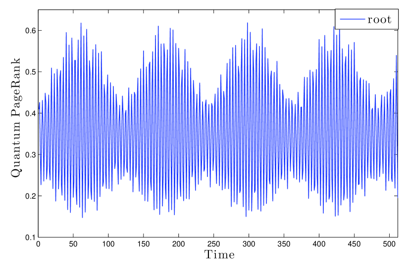
Figure 6: (Color online) The evolution of the instantaneous Quantum PageRank $I_{q}$ with time for the root page (home page) in the case of a directed binary tree in Fig.4.

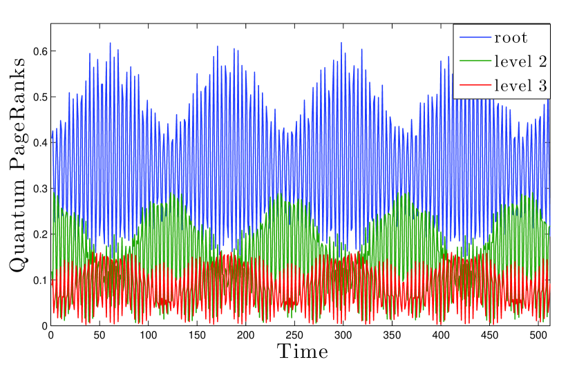
Figure 7: (Color online) The evolution with time of the instantaneous Quantum PageRank algorithm $I_{q}$ defined in Sect.IV for web pages (nodes) in the case of a directed binary tree graph in Fig.4. Only one page per level of the tree is displayed because pages that are in the same level have equal Quantum PageRank.

In order to extract a fixed value for the relative importances of the pages, we compute the mean value of the instantaneous quantum PageRank in time from eq. (35) and its variance from eq. (36).

One can notice that the hierarchy of the pages is preserved on average and that the errors i.e. the variances are negligible compared to the means. We can thus infer the pages’ hierarchy as predicted by the classical algorithm from the Quantum PageRanks’ averages as can be clearly seen in figure 8 for this particular case of directed binary tree graph.

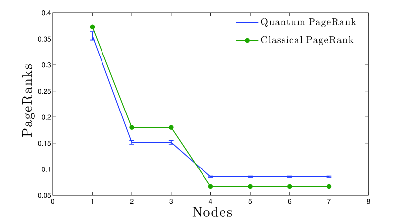
Figure 8: (Color online) Comparison of the hierarchies that result from the Classical and the Quantum PageRank in the case of the directed graph tree shown in Fig.4. Error bars in the quantum case are computed with the standard mean deviation (35),(36).

Level	Classical PageRank	Average Q-PageRank	Variance
1	0.37291	0.355905	0.0156461
2	0.18012	0.151437	0.0067747
3	0.06671	0.085305	0.0022797

Table 1: Comparison Classical and Averaged Q-PageRank in the case of the tree graph shown in Fig. 4. Given the symmetry of the tree only the values for each level are displayed.

Furthermore we can calculate a coarse grained evolution in time of the instantaneous Quantum PageRank. We divide its total evolution time of $M$ steps in $L$ equal segments made of an integer number $M/L$ steps. We calculate the mean in every segment:

$${\bar{I}_{q}(P_{i},n)}:=\frac{L}{M}\sum_{m=nM/L}^{(n+1)M/L-1}I_{q}(P_{i},m)\;,n=0,\ldots,L-1.$$ (37)

The result of integrating out the oscillations in a coarse grained time step is shown in figure 9. An interesting feature of this case is that the quantum PageRank oscillations shows a modulation with a clearly visible envelope for each node. It strongly enforces the idea that the proposed algorithm has a solid grounding on the classical PageRank algorithm and it is a valid quantization of it.

Figure 9: (Color online) The evolution in a coarse grained time (see text in section V) of the Quantum PageRanks in the case of the directed graph tree shown in Fig.4. Again only one page per level is being displayed because pages that are in the same level have equal Quantum PageRank.

V.2 Case Study 2: A General Graph

We have performed a calculation of the quantum PageRank also in the case of a general directed graph with no particular symmetry (see fig. 5).

The value of the instantaneous quantum PageRanks are found to display oscillations that are bounded and include the value found by the classical PageRank. The QPR of the node with the highest classical PageRank attains, at given times, values of the QPR that are higher than the classical counterpart (see fig. 10). As seen in the case of the binary tree treated above the Quantum PageRank is found to be instantaneously outperforming according to the definition given in section I.

The classical hierarchy is not preserved by the QPR at any given time (as is clearly shown by Fig. 10, see caption). We can notice crossings in the importance given by the instantaneous Quantum PageRank even between the pages that classically have highest and lowest PageRank. Furthermore, the nodes that have a very close classical PageRank are shown to have a very similar behaviour in time of their instantaneous Quantum PageRank.

Remarkably enough, we find that the Quantum PageRanks’ averages do not give us the same hierarchy as in the classical case (see Fig. 11). Nevertheless, it is possible to clearly distinguish, within the error bar given by the variance, which pages have highest and lowest classical PageRank.

The analysis with a coarse graining in time of the instantaneous Quantum PageRank (see Fig. 12) reinforces the conclusion that the classical PageRanks are still distillable in the case of pages with highest and lowest classical importances.

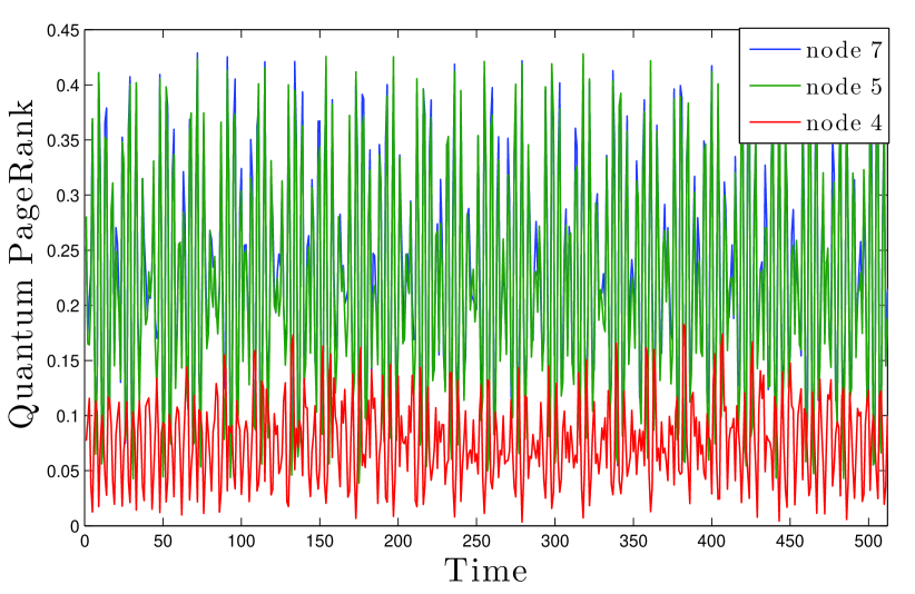
Figure 10: (Color online)The evolution in time of the Quantum PageRank $I_{q}$ of pages $7$, $5$ (that classically have the highest and nearly degenerate PageRank) and of page $4$ (that classically has the lowest PageRank) in the case of general graph shown in Fig.5.

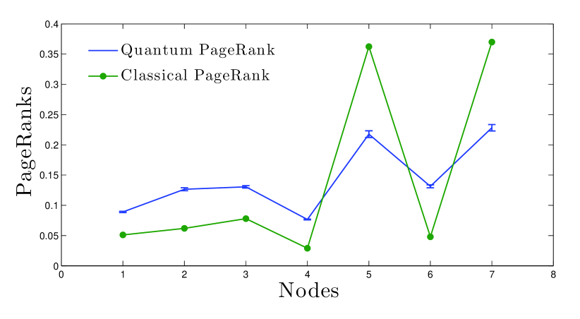
Figure 11: (Color online) Comparison of the hierarchies that result from the Classical and the Quantum PageRank in the case of the general graph shown in Fig.5. Error bars in the quantum case are computed with the standard mean deviation (35),(36).

Node	Classical PageRank	Average Q-PageRank	Variance
1	0.051019	0.089076	0.0021759
2	0.061860	0.126546	0.0050376
3	0.077924	0.130587	0.0040337
4	0.028940	0.076586	0.0014675
5	0.362387	0.217691	0.0111097
6	0.047981	0.131345	0.0049477
7	0.369889	0.228169	0.010549

Table 2: Comparison Classical and Averaged Q-PageRank in the case of the general graph shown in fig. 5.

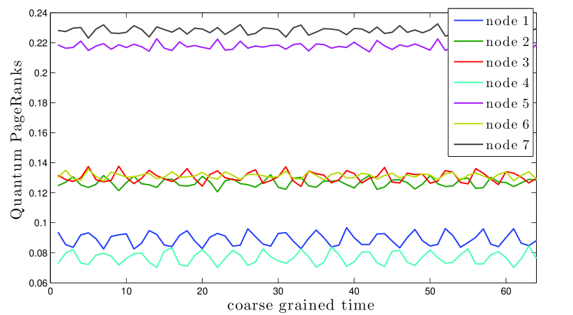
Figure 12: (Color online) The evolution in a coarse grained time (see text in section V) of the Quantum PageRanks in the case of the general graph shown in Fig.5.

VI Conclusions

In this paper we have proposed a notion of a class of protocols that qualify to be considered a quantum version of the classical PageRank algorithm employed by the Google search engine (see Sect.I). In addition, we have constructed a step-by-step protocol explicitly in Sect.IV based on the quantization of Markov chains for directed graphs. This is a non-trivial problem since dealing with quantum versions of digraphs may produce unitarity problems (see Sect.III). We have tested our quantum PageRank algorithm with two web networks in order to gain insight into the specific behaviour of this protocol. One network is a binary tree graph representing an intranet with the root being the home page of it. The other is a general directed graph with no specific structure.

From our numerical simulations we have found that our quantum PageRank has very interesting properties. For the directed binary tree:

i/ The quantum PageRank for the root page is instantaneously outperforming with respect to the classical value. This is a manifestation of the quantum fluctuations inherent to the quantum version of the algorithm and allows us to have an enhancement of the importance of the root page without changing the topology of the original network.

ii/ The instantaneous values of the quantum PageRanks for the nodes violate the hierarchy of the classical values.

iii/ The mean values of the quantum PageRanks including its standard deviation preserve the hierarchy of the classical values.

For the general directed graph:

i/ The quantum PageRank for the web page with the highest classical PageRank is some times higher than the classical values obtained with the standard algorithm. This means that the quantum version of the PageRank is instantaneously outperforming with respect to the classical value.

ii/ The instantaneous values of the quantum PageRanks for the nodes violate the hierarchy of the classical values.

iii/ Remarkably enough, there are pages with mean values, including its standard deviation, of their quantum PageRank that violate the hierarchy of the classical values.

These properties are a clear manifestation that our proposal for a quantum version of the PageRank algorithm exhibits nontrivial features with respect to the Classical PageRank.

As the main purpose of our work is to devise a quantum PageRank algorithm by overcoming certain difficulties explained in the paper, thus far we have dealt only with small networks representing different types of web. It would be very interesting to perform computations with the quantum PageRank applied to very large networks with the properties exhibited by the complex structure of the real web small-world ; scale-free ; self-similar1 ; self-similar2 ; statistical1 ; statistical2 ; deterministic .

An interesting issue is whether the classically first ranked page remains with the highest importance also at the quantum level. While we have shown that generically this is not the case for instantaneous values of the quantum PageRank (33) in Fig. 10 and Fig.13, they remain first-ranked with the time-average values of the quantum PageRank (35). It remains open to see what happens for larger networks having very similar first-ranked nodes when the effect of quantum fluctuations are taken into account. This will depend on the topology of the lattice as well.

- (1) C. Elliott; “The DARPA Quantum Network”; arXiv:quant-ph/0412029.
- (2) A. Poppe, M. Peev and O. Maurhart; “Outline of the SECOQC Quantum-Key-Distribution Network in Vienna ”; International Journal of Quantum Information Volume 6, 209-218 ( 2008).
- (3) Tokyo Quantum Network 2010. www.uqcc2010.org
- (4) Swiss Quantum Network. http://swissquantum.idquantique.com/
- (5) D. Lancho, J. Martinez, D. Elkouss, M. Soto and V. Martin; “QKD in Standard Optical Telecommunications Networks”; Lecture Notes of the Institute for Computer Sciences, Social Informatics and Telecommunications Engineering. Volume 36, pp 142-149 (2010). arXiv:1006.1858
- (6) T. Länger and G. Lenhart; “Standardization of quantum key distribution and the ETSI standardization initiative ISG-QKD”; New J. Phys. 11 055051 (2009).
- (7) M. A. Nielsen and I. L. Chuang, Quantum Computation and Quantum Information (Cambridge University Press, Cambridge, 2000).
- (8) A. Galindo and M.A. Martin-Delgado; “Information and Computation: Classical and Quantum Aspects”; Rev.Mod.Phys. 74:347-423, (2002); arXiv:quant-ph/0112105.
- (9) H. J. Kimble; “The quantum internet”; Nature (London) 453, 1023 (2008).
- (10) D. S. Wiersma; “Random Quantum Networks”; Science 327, 1333 (2010).
- (11) H.-J. Briegel, W. Dür, J.I. Cirac and P. Zoller; “Quantum Repeaters: The Role of Imperfect Local Operations in Quantum Communication”; Phys. Rev. Lett. 81, 5932 5935 (1998).
- (12) W. Dür, H.-J. Briegel, J.I. Cirac and P. Zoller; “Quantum repeaters based on entanglement purification”; Phys. Rev. A 59, 169 181 (1999).
- (13) N. Sangouard, Ch. Simon, H. de Riedmatten and N. Gisin; “Quantum repeaters based on atomic ensembles and linear optics”; Rev. Mod. Phys. 83, 33 80 (2011).
- (14) B. Lauritzen, J. Minar, H. de Riedmatten, M. Afzelius, and N. Gisin; “Approaches for a quantum memory at telecommunication wavelengths”; Phys. Rev. A 83, 012318 (2011).
- (15) C. Simon, M. Afzelius, J. Appel, A. Boyer de la Giroday, S.J. Dewhurst, N. Gisin, C.Y. Hu, F. Jelezko, S. Kroll, J.H. Muller, J. Nunn, E. Polzik, J. Rarity, H. de Riedmatten, W. Rosenfeld, A.J. Shields, N. Skold, R.M. Stevenson, R. Thew, I. Walmsley, M. Weber, H. Weinfurter, J. Wrachtrup, R.J. Young; “Quantum Memories. A Review based on the European Integrated Project ’Qubit Applications (QAP)”; The European Physical Journal D 58, 1-22 (2010).
- (16) B. Lauritzen, J. Minar, H. de Riedmatten, M. Afzelius, N. Sangouard, Ch. Simon and N. Gisin; “Telecommunication-Wavelength Solid-State Memory at the Single Photon Level”; Phys. Rev. Lett. 104, 080502 (2010).
- (17) F. Verstraete, M. A. Martin-Delgado and J. I. Cirac; “Diverging Entanglement Length in Gapped Quantum Spin Systems”; Phys. Rev. Lett. 92, 087201. arXiv:quant-ph/0311087.
- (18) M. Popp, F. Verstraete, M.A. Martin-Delgado and J. I. Cirac; “Localizable entanglement”; Phys. Rev. A 71, 042306 (2005). arXiv:quant-ph/0411123.
- (19) V.E. Korepin and Ying Xu, “Entanglement in Valence-Bond-Solid States”; International Journal of Modern Physics B 24, pp. 1361-1440 (2010).
- (20) M. Hein, W. Dür, J. Eisert, R. Raussendorf, M. Van den Nest, H.-J. Briegel; “Entanglement in Graph States and its Applications”; Proceedings of the International School of Physics “Enrico Fermi” on “Quantum Computers, Algorithms and Chaos”, Varenna, Italy, July, 2005. arXiv:quant-ph/0602096.
- (21) A. Acin, J.I. Cirac and M. Lewenstein; “Entanglement percolation in quantum networks”; Nature Physics 3, 256 - 259 (2007).
- (22) S. Perseguers, J.I. Cirac, A. Acin, M. Lewenstein and Jan Wehr; “Entanglement distribution in pure-state quantum networks”; Phys. Rev. A 77, 022308 (2008).
- (23) M.Cuquet and J. Calsamiglia; “Entanglement Percolation in Quantum Complex Networks”; Phys. Rev. Lett. 103, 240503 (2009).
- (24) M.Cuquet and J. Calsamiglia; “Limited-path-length entanglement percolation in quantum complex networks”; Phys. Rev. A 83, 032319 (2011).
- (25) S. Brin, L. Page; “The anatomy of a large-scale hypertextual Web search engine”; Computer Networks and ISDN Systems 33 (1998) 107-17.
- (26) S. Brin, R. Motwami, L. Page, T. Winograd; “What can you do with a web in your pocket?”; Data Engineering bulletin 21 (1998) 37-47.
- (27) S. Brin, R. Motwami, L. Page, T. Winograd; “The PageRank Citation Ranking: Bringing order to the Web”; Technical Report, Computer Science Department, Stanford University (1998).
- (28) A. Langville, C. Meyer; “Deeper Inside PageRank”; Internet Mathematics Vol. I, 3 (2004) 335-380.
- (29) C.D. Meyer; Matrix Analysis and Applied Linear Algebra Philadelphia, PA SIAM (2000).
- (30) T. Haveliwala, S. Kamvar; “The Second Eigenvalue of the Google Matrix”; Stanford University Technical Report, 2003-20 (2003).
- (31) A. Arratia and C. Marijuan;“Ranking pages and the topology of the web”; arXiv:1105.1595.
- (32) B. Georgeot, O. Giraud and D.L. Shepelyansky; “Spectral properties of the Google matrix of the World Wide Web and other directed networks”. Phys. Rev. E 81, 056109 (2010).
- (33) R. Cilibrasi and P. M. B. Vitanyi; “The Google Similarity Distance”; IEEE Trans. Knowledge and Data Engineering, 19:3 (2007), 370-383
- (34) R. P. Feynman and A. R. Hibbs; Quantum mechanics and path integrals. International series in pure and applied physics (McGraw-Hill, New York, 1965).
- (35) Y. Aharonov, L. Davidovich, and N. Zagury; “Quantum random walks” Phys. Rev. A, 48(2) : 1687 1690 (1993).
- (36) D. Meyer; “From quantum cellular automata to quantum lattice gases”; J. Stat. Phys., 85, 551 574 (1996).
- (37) D. Meyer; “On the absence of homogeneous scalar unitary cellular automata”; Phys. Lett. A, 223(5), 337 340, 1996.
- (38) J. Watrous; “Quantum simulations of classical random walks and undirected graph connectivity”; Journal of Computer and System Sciences, 62(2), 376 391 (2001).
- (39) M.A. Martin-Delgado; “Alan Turing and the Origins of Complexity”; arXiv:1110.0271.
- (40) M. Szegedy; “Quantum Speed-up of Markov Chain Based Algorithms”; Proceedings of the 45th Annual IEEE Symposium on Foundations of Computer Science (2004), pp. 32-41.
- (41) S. Garnerone, P. Zanardi, D. A. Lidar; “Adiabatic quantum algorithm for search engine ranking”; arXiv:1109.6546.
- (42) D.J. Watts and S.H. Strogatz, “Collective dynamics of ’small-world’ networks”; Nature 393 409, (1998).
- (43) A.-L. Barabási and R. Albert; “Emergence of scaling in random networks”; Science 286 509, (1999).
- (44) C. Song, S. Havlin and H. A. Maksé; “Self-similarity of Complex Networks”; Nature 433 392, (2005).
- (45) E. Ravasz, A. L. Somera, D. A. Mongru, Z.N. Oltvai and A.-L. Barabási; “Hierarchical Organization of Modularity in Metabolic Networks”; Science 297 1551, (2002).
- (46) R. Albert, A.-L. Barabási; “Statistical mechanics of complex networks”; Rev. Mod. Phys. 74 47-97, (2002).
- (47) M.E.J. Newman; “The structure and function of complex networks”; SIAM Rev. 45 167 256, (2003).
- (48) F. Comellas, J. Ozón and J.G. Peters; “Deterministic small-world communication networks”; Inform. Proc. Lett. 76 83 90, (2000).