A stochastic approach to the solution of magnetohydrodynamic equations

Abstract

The construction of stochastic solutions is a powerful method to obtain localized solutions in configuration or Fourier space and for parallel computation with domain decomposition. Here a stochastic solution is obtained for the magnetohydrodynamics equations. Some details are given concerning the numerical implementation of the solution which is illustrated by an example of generation of long-range magnetic fields by a velocity source.

Keywords: Kinetic equations, Stochastic solutions, Magnetohydrodynamics

1 Introduction

To solve complex differential problems in large domains, one way to profit from parallel computation in multiprocessor machines is to decompose the domain into subdomains and assign the problem in each subdomain to a different processor. However, one is left with the problem of computation of the boundary conditions in the subdomain interfaces. This implies that, in addition to the time consumed solving the equation in each subdomain, a considerable amount of time will also be consumed in the communication between processors. The ideal situation would be to have a method to compute local solutions at the interface points without the need for a grid. Such a method is implicit in the idea of stochastic solutions.

In the following the notion of stochastic solution is introduced for linear partial differential equations and a method is described that extends this notion to nonlinear equations. In addition to its use in domain decomposition problems, other relevant features of the stochastic solutions are discussed.

1.1 The notion of stochastic solution: Linear and nonlinear partial differential equations

Linear elliptic and parabolic equations (both with Cauchy and Dirichlet boundary conditions) have a probabilistic interpretation. This is a classical result and a standard tool in potential theory. As a simple example consider the heat equation

$$\frac{\partial}{\partial t}u(t,x)=\frac{1}{2}\frac{\partial^{2}}{\partial x^{2}}u(t,x)\qquad\text{with}\qquad u(0,x)=f(x)$$ (1)

The solution may be written either as

$$u\left(t,x\right)=\frac{1}{\sqrt{2\pi}}\int\frac{1}{\sqrt{t}}\exp\left(-\frac{\left(x-y\right)^{2}}{2t}\right)f\left(y\right)dy$$ (2)

or as

$$u(t,x)=\mathbb{E}_{x}f(X_{t})$$ (3)

$\mathbb{E}_{x}$ being the expectation value, starting from $x$, of the Wiener process $dX_{t}=dW_{t}$.

Whereas Eq.(1) is a specification of the problem, Eqs.(2) and (3) are solutions in the sense that they both provide algorithms for the construction of a function satisfying the specification. An important condition for (2) and (3) to be considered as solutions is the fact that the algorithm is independent of the particular solution, in the first case an integration procedure and in the second a solution-independent process. This should be contrasted with stochastic processes constructed from a given particular solution, as has been done, for example, for the Boltzmann equation.

Whenever a similar stochastic process algorithm may be associated to nonlinear equations, this would provide new exact solutions and new numerical algorithms. To obtain stochastic solutions for nonlinear equations, it is useful to recall that in the linear partial differential equation case the stochastic process starts from the point $x$ where the solution is to be computed and the solution is a functional of the exit values of the process (from a space domain $D$ or a space-time domain $D\times\left[0,t\right]$). Therefore, it is natural to conjecture that for the nonlinear equations the relevant process would have a diffusion, propagation or jump component associated to the linear part of the equation plus a branching mechanism associated to the nonlinear part. Then the solution would also be a functional of the exit measures generated by the process.

For the implementation of this conjecture one rewrites the equation as an integral one, for which a probabilistic interpretation is given. In the end the stochastic solution is the expectation of a functional over a tree-indexed measure. The method, which leads to rigorous results, may also be looked at, in qualitative terms, as importance sampling evaluation of the Picard series.

This method was first used in the pioneering paper of McKean [1] for the Kolmogorov-Petrovskii-Piskonov (KPP) equation. Later, a similar technique was used for the Navier-Stokes [2] [3], the Vlasov-Poisson [4] [5] [6] [8], the Euler [7] and a fractional version of the KPP equation [9]. For the diffusion equation with $u^{\alpha}$ $\left(\alpha\in\left[0,2\right]\right)$ nonlinearities, Dynkin uses a different method [10], namely scaling limits leading to superprocesses (for a comparison of the McKean-type construction and superprocesses see [11]).

1.2 Stochastic solutions and numerical algorithms

Once a stochastic solution is obtained for a partial differential equation, how does it stand in comparison with deterministic numerical algorithms? The main points to be considered are:

(a) Stochastic solutions may provide new exact solutions in cases where exact solutions were not known before.

(b) Deterministic algorithms grow exponentially with the dimension $d$ of the space, roughly $N^{d}$ ($\frac{L}{N}$ being the linear size of the grid) whereas the numerical implementation of a stochastic process only grows with the dimension $d$.

(c) Deterministic algorithms aim at obtaining the solution in the whole domain. Then, even if an efficient deterministic algorithm exists, the stochastic algorithm might still be competitive if only localized values of the solution are desired. For example by studying only a few high Fourier modes one may obtain information on the small scale fluctuations which would require a very fine grid in a deterministic algorithm.

(d) Each sample path of the stochastic process is independent of the others. Likewise, paths starting from different points are independent from each other. Therefore the stochastic algorithms are a natural choice for parallel and distributed computation.

(e) Stochastic algorithms handle equally well regular and complex boundary conditions although, of course, the computation of exit times from complex domains might not be an easy matter.

(f) Also, as already pointed out, the local nature of the stochastic solutions make them the most appropriate choice to obtain boundary conditions in subdomain interfaces, thus avoiding the time consuming communication problem. The remarkable efficiency of this method for domain decomposition schemes has been described in [12] [13] [14].

2 Stochastic solutions of magnetohydrodynamics equations

Magnetohydrodynamics concerns the dynamics of magnetic fields in electrically conducting fluids, e.g. plasmas or liquid metals. It is a macroscopic theory which may be considered as an approximation of the Boltzmann’s equation when the space and time scales are larger than all relevant length scales, such as the Debye length or the gyro-radius of the charged particles. We consider, in a non-relativistic approximation, the equations of magnetohydrodynamics in 3 dimensions, with non-zero fluid viscosity and electric resistivity. The fluid is taken to be incompressible with density $\rho(x,t)=\rho_{0}$ constant and uniform. The equations for the velocity $\overset{\rightarrow}{V}(x,t)$ of the fluid and the magnetic field $\overset{\rightarrow}{B}(x,t)$ are:

$$\frac{\partial\overset{\rightarrow}{V}}{\partial t}=-(\overset{\rightarrow}{V}\cdot\nabla)\overset{\rightarrow}{V}+\frac{1}{\rho_{0}\mu_{0}}(\overset{\rightarrow}{B}\cdot\nabla)\overset{\rightarrow}{B}-\frac{1}{2\rho_{0}\mu_{0}}\nabla\overset{\rightarrow}{B}^{2}-\frac{1}{\rho_{0}}\nabla P+\nu\nabla^{2}\overset{\rightarrow}{V}+\overset{\rightarrow}{F}(x,t)$$ (4)

$$\frac{\partial\overset{\rightarrow}{B}}{\partial t}=-(\overset{\rightarrow}{V}\cdot\nabla)\overset{\rightarrow}{B}+(\overset{\rightarrow}{B}\cdot\nabla)\overset{\rightarrow}{V}+\frac{\eta}{\mu_{0}}\nabla^{2}\overset{\rightarrow}{B}$$ (5)

$\nu$ being the kinematic viscosity, $\eta$ the resistivity and $\mu_{0}$ the vacuum permeability. $\overset{\rightarrow}{F}(x,t)$ is a forcing term for the fluid velocity. For the Fourier transformed quantities,

$$\overset{\rightarrow}{v}(k,t) = (2\pi)^{-3/2}\int d^{3}x\,\overset{\rightarrow}{V}(x,t)\,e^{ik\cdot x}$$

$$\overset{\rightarrow}{b}(k,t) = (2\pi)^{-3/2}\int d^{3}x\,\overset{\rightarrow}{B}(x,t)\,e^{ik\cdot x}$$

$$\overset{\rightarrow}{f}(k,t) = (2\pi)^{-3/2}\int d^{3}x\,\overset{\rightarrow}{F}(x,t)\,e^{ik\cdot x}$$

use the fact that the divergences of $\overset{\rightarrow}{V}(x,t),\overset{\rightarrow}{B}(x,t),\overset{\rightarrow}{F}(x,t)$ vanish and project on the plane orthogonal to the vector $k$. The projection operator is

$$\pi_{(k)}(\overset{\rightarrow}{\xi})=\overset{\rightarrow}{\xi}-(\overset{\rightarrow}{\xi}\cdot\overset{\rightarrow}{e_{k}})\overset{\rightarrow}{e_{k}}$$

with $e_{k}=\frac{k}{|k|}$. The projection eliminates the gradient terms and, since $k\cdot v(k,t)=k\cdot b(k,t)=0$, no information is lost on the velocity and magnetic fields. Then we obtain

$$\frac{\partial\overset{\rightarrow}{v}(k,t)}{\partial t} = -\nu k^{2}\overset{\rightarrow}{v}(k,t)+(2\pi)^{-3/2}|k|\,\int d^{3}q\,\left\{\overset{\rightarrow}{v}(q,t)\otimes_{k}\overset{\rightarrow}{v}(k-q,t)\right.$$ (6)

$$\left.-\frac{1}{\rho_{0}\mu_{0}}\,\overset{\rightarrow}{b}(q,t)\otimes_{k}\overset{\rightarrow}{b}(k-q,t)\right\}+\overset{\rightarrow}{\varphi}(k,t)$$

$$\frac{\partial\overset{\rightarrow}{b}(k,t)}{\partial t} = -\,\frac{\eta}{\mu_{0}}k^{2}\overset{\rightarrow}{b}(k,t)+(2\pi)^{-3/2}|k|\,\int d^{3}q\,\left\{\overset{\rightarrow}{v}(q,t)\otimes_{k}\overset{\rightarrow}{b}(k-q,t)\right.$$ (7)

$$\left.-\overset{\rightarrow}{b}(q,t)\otimes_{k}\overset{\rightarrow}{v}(k-q,t)\right\}$$

where $\overset{\rightarrow}{\varphi}(k,t)=\pi_{(k)}\overset{\rightarrow}{f}(k,t)$ is the Fourier transform of the divergenceless part of the forcing and the product $\otimes_{k}$ between two vectors $\overset{\rightarrow}{\xi},\overset{\rightarrow}{\omega}$ is defined by

$$\overset{\rightarrow}{\xi}\otimes_{k}\overset{\rightarrow}{\omega}=i(\overset{\rightarrow}{e_{k}}\cdot\overset{\rightarrow}{\xi})\,\pi_{(k)}\overset{\rightarrow}{\omega}$$ (8)

The next step will be to give a probabilistic interpretation to the magnetohydrodynamics equations by defining a process and an associated functional that provides the solution. Two constructions will be given. They both lead to rigorous results. However, for practical purposes and numerical implementation the one that is most convenient will depend on the values of the equation physical parameters.

2.1 Dissipation-controlled stochastic clock

To guarantee convergence of the functionals associated to the stochastic processes it is convenient to rescale the vectors $\overset{\rightarrow}{v}(k,t)$ and $\overset{\rightarrow}{b}(k,t)$ by a $k-$dependent function $h(k)$. This rescaling should be familiar from the convergence proofs of Picard iteration and will also be called the majorizing kernel. Define:

$$\overset{\rightarrow}{\chi_{v}}(k,t)=\frac{\overset{\rightarrow}{v}(k,t)}{h(k)}\;,\;\;\;\;\;\;\overset{\rightarrow}{\chi_{b}}(k,t)=\frac{\overset{\rightarrow}{b}(k,t)}{\sqrt{\rho_{0}\mu_{0}}\;h(k)}$$ (9)

Then the integral equations equivalent to (6-7) are:

$$\overset{\rightarrow}{\chi_{v}}(k,t) = \overset{\rightarrow}{\chi_{v}}(k,0)e^{-\nu k^{2}t}+\int_{0}^{+\infty}ds\,\nu k^{2}\,e^{-\nu k^{2}s}\left\{\frac{1}{3}\overset{\rightarrow}{\rho}(k,t-s)+\int d^{3}q\frac{h(q)h(k-q)}{(h\ast h)(k)}\right.$$ (10)

$$\left[\frac{1}{3}\,g_{v\rightarrow vv}(k)\,\overset{\rightarrow}{\chi_{v}}(q,t-s)\otimes_{k}\overset{\rightarrow}{\chi_{v}}(k-q,t-s)+\right.$$

$$\left.\left.\frac{1}{3}\,g_{v\rightarrow bb}(k)\overset{\rightarrow}{\chi_{b}}(q,t-s)\otimes_{k}\overset{\rightarrow}{\chi_{b}}(k-q,t-s)\right]\right\}$$

and

$$\overset{\rightarrow}{\chi_{b}}(k,t) = \overset{\rightarrow}{\chi_{b}}(k,0)e^{-\frac{\eta}{\mu_{0}}\,k^{2}t}+\int_{0}^{+\infty}ds\,\frac{\eta}{\mu_{0}}\,k^{2}\,e^{-\frac{\eta}{\mu_{0}}\,k^{2}s}\int d^{3}q\,\frac{h(q)h(k-q)}{(h\ast h)(k)}$$ (11)

$$\left\{\frac{1}{2}\,g_{b\rightarrow vb}(k)\,\overset{\rightarrow}{\chi_{v}}(q,t-s)\otimes_{k}\overset{\rightarrow}{\chi_{b}}(k-q,t-s)+\right.$$

$$\left.\frac{1}{2}\,g_{b\rightarrow bv}(k)\,\overset{\rightarrow}{\chi_{b}}(q,t-s)\otimes_{k}\overset{\rightarrow}{\chi_{v}}(k-q,t-s)\right\}\,$$

with the functions $g_{\ast\rightarrow\ast\ast}$ and $\overset{\rightarrow}{\rho}$ defined by:

$$g_{v\rightarrow vv}(k) = -g_{v\rightarrow bb}(k)=\frac{3(2\pi)^{-3/2}(h\ast h)(k)}{\nu\,|k|\,h(k)}$$

$$g_{b\rightarrow vb}(k) = -g_{b\rightarrow bv}(k)=\frac{2(2\pi)^{-3/2}\mu_{0}\,(h\ast h)(k)}{\eta\,|k|\,h(k)}$$

$$\overset{\rightarrow}{\rho}(k,t) = \frac{3\,\overset{\rightarrow}{\varphi}(k,t)}{\nu k^{2}h(k)}$$ (12)

The equations (10), (11) have a probabilistic interpretation as two coupled stochastic processes which combine exponential decay and branching. For the exponential processes $\,\left[e^{-\nu k^{2}t}\right]\,$ and $\,\left[e^{-(\eta/\mu_{0})k^{2}t}\right]\,$ are the survival probabilities up to time $t$ and $\,\left[\nu k^{2}\,e^{-\nu k^{2}s}\,ds\right]\,$ and $\,\left[(\eta/\mu_{0})k^{2}\,e^{-(\eta/\mu_{0})k^{2}s}\,ds\right]\,$ are the decay probabilities in the time interval $(s,s+ds)$. On the other hand $\left[\,h(q)h(k-q)/(h\ast h)(k)\,d^{3}q\right]\,$ is the probability that, given a $k$ mode, one obtains a branching to modes $q,k-q$. The possible branches, three for $\overset{\rightarrow}{\chi_{v}}(k,t)$ and two for $\overset{\rightarrow}{\chi_{b}}(k,t)$, are selected with equal probabilities $\left(\frac{1}{3},\frac{1}{3},\frac{1}{3}\right)$ and $\left(\frac{1}{2},\frac{1}{2}\right)$. The functions $g_{\ast\rightarrow\ast\ast}$ play the role of coupling constants at the branching points and $\overset{\rightarrow}{\rho}$ is a source term.

To obtain $\overset{\rightarrow}{\chi_{v}}(k,t)$ and$\,\overset{\rightarrow}{\chi_{b}}(k,t)$ the processes are iterated backwards in time from time $t$ to time zero. Then, for each realization, starting from the values of the initial conditions that are reached at time zero or from the source terms, one reconstructs the values at time $t$ following the process forward in time and multiplying at each vertex by the appropriate coupling constant $g_{\ast\rightarrow\ast\ast}$, with the appropriate product $\otimes_{k}$($k$ being the Fourier argument at that vertex). The solutions $\overset{\rightarrow}{\chi_{v}}(k,t)$ and$\,\overset{\rightarrow}{\chi_{b}}(k,t)$ are the expectation values of this process, obtained by averaging over many realizations. In Fig.1 we show a typical sample path of the $\overset{\rightarrow}{\chi_{b}}(k,t)$ process. The backwards-in-time process, starts from the time $t$ at which the solution is to be computed and runs to time zero, except when a source term is sampled, which stops that particular branch of the process.

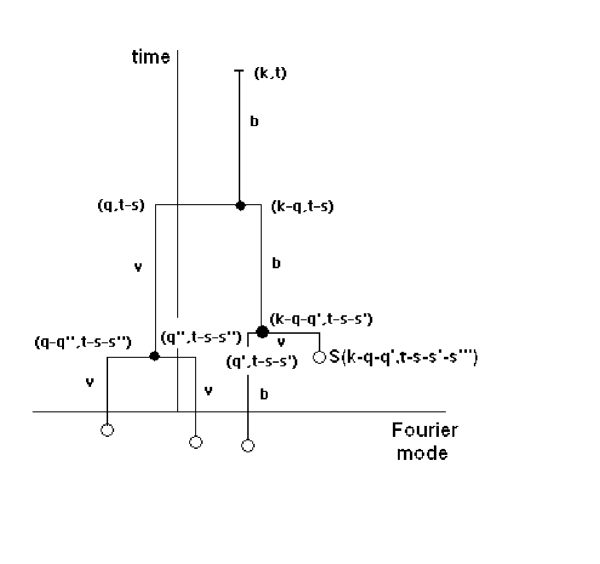
Figure 1: A sample path of the $\chi_{b}(k,t)$ process

With the probability structure as defined above, the branching process, being identical to a Galton-Watson process, terminates with probability one and the number of inputs to the calculation of $\overset{\rightarrow}{\chi_{v}}(k,t)$ and$\,\overset{\rightarrow}{\chi_{b}}(k,t)$ is finite (with probability one). The following bounds are imposed:

- On the coupling constants:

$$g_{\ast\rightarrow\ast\ast}(k)\leq 1\;\;\;\;\;\;\Longleftrightarrow\;\;\;\;\;\;3(2\pi)^{-3/2}(h\ast h)(k)\leq\min\left(\nu,\frac{\eta}{\mu_{0}}\right)\,|k|\,h(k)$$ (13)

- On the source term:

$$\left|\overset{\rightarrow}{\rho}(k,t)\right|\leq 1\;\;\;\;\;\;\Longleftrightarrow\;\;\;\;\;\;\left|\overset{\rightarrow}{\varphi}(k,t)\right|\leq\frac{\nu k^{2}h(k)}{3}\;\;\forall t$$ (14)

- On the initial conditions:

$$\left|\overset{\rightarrow}{\chi_{v}}(k,0)\right|\leq 1;\;\;\left|\overset{\rightarrow}{\chi_{b}}(k,0)\right|\leq 1\;\;\;\;\;\;\Longleftrightarrow\;\;\;\;\;\;\left|\overset{\rightarrow}{v}(k,0)\right|\leq h(k);\;\left|\overset{\rightarrow}{b}(k,0)\right|\leq\sqrt{\rho_{0}\mu_{0}}\;h(k)$$ (15)

Provided the bounds (13)-(15) on the couplings, the forcing and the initial conditions are satisfied, the expectation values of $\overset{\rightarrow}{\chi_{v}}$ and $\overset{\rightarrow}{\chi_{b}}$ are bounded by one in absolute value almost surely. Once a stochastic solution is obtained for $\overset{\rightarrow}{\chi_{v}}(k,t)$ and $\overset{\rightarrow}{\chi_{b}}(k,t)$, one also has, by (9), stochastic solutions for $\overset{\rightarrow}{v}(k,t)$ and $\overset{\rightarrow}{b}(k,t)$. Summarizing:

Proposition 1 The stochastic processes $\overset{\rightarrow}{\chi_{v}}(k,t)$ and $\overset{\rightarrow}{\chi_{b}}\left(k,t\right)$, above described, provide stochastic solutions to the magnetohydrodynamics equations, existence of such solutions being guaranteed by the bounds (13)-(15).

This being a rigorous result, the mean value over many realizations of the process will provide a solution of the magnetohydrodynamics equations. However, one notices that if $\nu$ and $\frac{\eta}{\mu_{0}}$ are small, as they indeed are in many situations of practical interest, then for short or moderate times most process trees have no branching at all. Hence all the contributions related to nonlinear effects are concentrated in just a few exceptional multibranch trees. This is a typical large deviation situation, which is even more serious than usual because with the $\leq 1$ bounds on the couplings we would like to be able to neglect the contributions of large multibranch trees. To avoid this large deviation problem, when $\nu$ and $\frac{\eta}{\mu_{0}}$ are small, the stochastic clock should be changed. This we do in the next subsection, where another rigorous solution representation is constructed using an externally defined stochastic branching clock.

2.2 Externally defined stochastic clock

Here we use a time-dependent majorizing kernel

$$\overset{\rightarrow}{\varsigma_{v}}(k,t)=\frac{\overset{\rightarrow}{v}(k,t)}{e^{\lambda t}h(k)}\;,\;\;\;\;\;\;\overset{\rightarrow}{\varsigma_{b}}(k,t)=\frac{\overset{\rightarrow}{b}(k,t)}{e^{\lambda t}\sqrt{\rho_{0}\mu_{0}}\;h(k)}$$ (16)

with $\lambda$ a positive real number. The integral equations for these quantities are:

$$\overset{\rightarrow}{\varsigma_{v}}(k,t) = \overset{\rightarrow}{\varsigma_{v}}(k,0)e^{-\left(\lambda+\nu k^{2}\right)t}+\int_{0}^{+\infty}ds\,\left(\lambda+\nu k^{2}\right)e^{-\left(\lambda+\nu k^{2}\right)s}\left\{\frac{1}{3}\overset{\rightarrow}{\sigma}(k,t-s)+\int d^{3}q\frac{h(q)h(k-q)}{(h\ast h)(k)}\right.$$ (17)

$$\left[\frac{1}{3}\,\gamma_{v\rightarrow vv}(k,t-s)\,\overset{\rightarrow}{\varsigma_{v}}(q,t-s)\otimes_{k}\overset{\rightarrow}{\varsigma_{v}}(k-q,t-s)+\right.$$

$$\left.\left.\frac{1}{3}\,\gamma_{v\rightarrow bb}(k,t-s)\overset{\rightarrow}{\varsigma_{b}}(q,t-s)\otimes_{k}\overset{\rightarrow}{\varsigma_{b}}(k-q,t-s)\right]\right\}$$

$$\overset{\rightarrow}{\varsigma_{b}}(k,t) = \overset{\rightarrow}{\varsigma_{b}}(k,0)e^{-\left(\lambda+\frac{\eta}{\mu_{0}}k^{2}\right)t}+\int_{0}^{+\infty}ds\,\left(\lambda+\frac{\eta}{\mu_{0}}k^{2}\right)\thinspace e^{-\left(\lambda+\frac{\eta}{\mu_{0}}k^{2}\right)s}\int d^{3}q\,\frac{h(q)h(k-q)}{(h\ast h)(k)}$$ (18)

$$\left\{\frac{1}{2}\,\gamma_{b\rightarrow vb}(k,t-s)\,\overset{\rightarrow}{\varsigma_{v}}(q,t-s)\otimes_{k}\overset{\rightarrow}{\varsigma_{b}}(k-q,t-s)+\right.$$

$$\left.\frac{1}{2}\,\gamma_{b\rightarrow bv}(k,t-s)\,\overset{\rightarrow}{\varsigma_{b}}(q,t-s)\otimes_{k}\overset{\rightarrow}{\varsigma_{v}}(k-q,t-s)\right\}\,$$

with

$$\gamma_{v\rightarrow vv}(k,t) = -\gamma_{v\rightarrow bb}(k,t)=\frac{3e^{\lambda t}\,|k|(h\ast h)(k)}{(2\pi)^{3/2}\left(\lambda+\nu k^{2}\right)\,h(k)}$$

$$\gamma_{b\rightarrow vb}(k,t) = -\gamma_{b\rightarrow bv}(k,t)=\frac{2e^{\lambda t}|k|(h\ast h)(k)}{(2\pi)^{3/2}\left(\lambda+\frac{\eta}{\mu_{0}}k^{2}\right)\,\,h(k)}$$

$$\overset{\rightarrow}{\sigma}(k,t) = \frac{3\,e^{-\lambda t}\overset{\rightarrow}{\varphi}(k,t)}{\left(\lambda+\nu k^{2}\right)h(k)}$$ (19)

The stochastic processes associated to (17) and (18) are identical to those of (10) and (11). A sufficient condition for convergence of the processes is, as before, assured by keeping the magnitude of all contributions $\leq 1$ which, together with the fact that the process finishes in finite time with probability one, guarantees convergence. This is fulfilled by the following bounds:

- On the coupling constants:

$$\gamma_{*\rightarrow**}(k,t)\leq 1\;\;\Longleftrightarrow\;\;3(2\pi)^{-3/2}e^{\lambda t}|k|(h\ast h)(k)\leq\,\left(\lambda+\min\left(\nu,\frac{\eta}{\mu_{0}}\right)k^{2}\right)\,h(k)\;\;\;\;\forall t$$ (20)

- On the source term:

$$\left|\overset{\rightarrow}{\sigma}(k,t)\right|\leq 1\;\;\;\;\Longleftrightarrow\;\;\;\;\left|\overset{\rightarrow}{\varphi}(k,t)\right|\leq\frac{\left(\lambda+\nu k^{2}\right)h(k)}{3}e^{\lambda t}\;\;\;\;\forall t$$ (21)

- On the initial conditions:

$$\left|\overset{\rightarrow}{\varsigma_{v}}(k,0)\right|\leq 1;\;\;\left|\overset{\rightarrow}{\varsigma_{b}}(k,0)\right|\leq 1\;\;\;\;\Longleftrightarrow\;\;\;\;\left|\overset{\rightarrow}{v}(k,0)\right|\leq h(k);\;\;\left|\overset{\rightarrow}{b}(k,0)\right|\leq\sqrt{\rho_{0}\mu_{0}}\;h(k)$$ (22)

In conclusion:

Proposition 2 The stochastic processes $\overset{\rightarrow}{\varsigma_{v}}(k,t)$ and $\overset{\rightarrow}{\varsigma_{b}}\left(k,t\right)$, above described, provide stochastic solutions to the magnetohydrodynamics equations, existence of such solutions being guaranteed by the bounds (20)-(22).

In contrast with the previous solution where the clock is purely dissipation-controlled, now the bounds are explicitly time-dependent, meaning that the longer $t$ is, the more stringent are the bounds on the majorizing kernel and therefore the smaller must be the initial conditions. Therefore this solution provides only finite-time solutions and, if longer timer are desired for fixed initial conditions, successive finite-time solutions should be patched up.

This solution provides implementations where the nonlinear effects are easier to put in evidence. However, if the dissipation is extremely small the solution is not yet fully satisfactory as far as the large deviation problem is concerned. This comes about because the most favorable existing kernels being those that satisfy either

$$(h\ast h)(k)\leq\left|k\right|\,\,h(k)$$ (23)

or

$$(h\ast h)(k)\leq h(k)$$ (24)

inspection of (20) implies that it is always $\min\left(\nu,\frac{\eta}{\mu_{0}}\right)$ that controls the magnitude of the kernel. Therefore to handle the extremely small dissipation case it would be better to construct a solution that applies also in the non-dissipative case $\left(\nu=\eta=0\right)$. Of course, in the non-dissipative case we will have the same limitations as in the construction of the finite-time solutions of the three-dimensional Euler equation (see, for example Sect.2.5 in [15]). As before define

$$\overset{\rightarrow}{\varsigma_{v}}(k,t)=\frac{\overset{\rightarrow}{v}(k,t)}{e^{\lambda t}h(k)}\;,\;\;\;\;\;\;\overset{\rightarrow}{\varsigma_{b}}(k,t)=\frac{\overset{\rightarrow}{b}(k,t)}{e^{\lambda t}\sqrt{\rho_{0}\mu_{0}}\;h(k)}$$ (25)

but we restrict both the initial condition and the kernel to a maximum momentum $\left|k\right|=k_{M}$, that is

$$\overset{\rightarrow}{\varsigma_{v}}(k,0)=\overset{\rightarrow}{\varsigma_{b}}(k,0)=0\;,\;\;\;\;\;\;h\left(k\right)=0\;\;\;\;\;\;\text{ if }\left|k\right|>k_{M}$$ (26)

The integral evolution equations are the same as before ((17) and (18)). The branching probability being

$$p\left(k-q,q\right)=\frac{h(q)h(k-q)}{(h\ast h)(k)}$$ (27)

no new branches are created with $\left|k\right|>k_{M}$. Therefore this choice of kernel effectively projects the equation on the subspace of momentum $\left|k\right|<k_{M}$. Because in the final computation of the functional leading to the solution only the ratios $\frac{\overset{\rightarrow}{v}(k,0)}{h(k)}$ and $\frac{\overset{\rightarrow}{b}(k,0)}{h(k)}$ intervene, consistency is maintained as long as the initial conditions satisfy (26).

In the non-dissipative limit the bound (20) becomes

$$3(2\pi)^{-3/2}e^{\lambda t}(h\ast h)(k)\leq\,\frac{\lambda}{k_{M}}h(k)$$

A general finite-time solution is obtained by a sequence of stochastic processes corresponding to successively larger $k_{M}^{\prime}$ s.

In the next section we will provide some details on how to implement the bounds (13)-(15) and (20)-(22) as well as the branching probabilities which are then illustrated by an example showing the generation of long-range magnetic fields by a velocity source.

3 Kernel and branching probabilities for the numerical implementation of the solutions

3.1 A majorizing kernel and the bounds

As we have seen before, convergence of the processes requires:

$$|k|(h\ast h)(k)\leq\,\gamma\left(\lambda+\min\left(\nu,\frac{\eta}{\mu_{0}}\right)k^{2}\right)\,h(k)$$ (28)

($\lambda=0$ for proposition 1). That means

$$(h\ast h)(k)\leq\gamma^{\prime}\min\left(\nu,\frac{\eta}{\mu_{0}}\right)|k|h(k)$$ (29)

for the cases with dissipation and

$$|k|(h\ast h)(k)\leq\gamma^{\prime\prime}\lambda\,h(k)$$ (30)

in the non-dissipative limit.

The following majorizing kernel

$$h\left(k\right)=\frac{c}{\left|k\right|^{2}}$$ (31)

satisfies (29). Indeed, from

$$\int d^{3}k^{\prime}\frac{1}{\left|k-k^{\prime}\right|^{2}}\frac{1}{\left|k^{\prime}\right|^{2}}=\frac{\pi^{3}}{\left|k\right|}$$

one concludes that (29) holds if

$$c\leq\frac{\gamma^{\prime}\min\left(\nu,\frac{\eta}{\mu_{0}}\right)}{\pi^{3}}$$

We now discuss the bounds (13)-(15) for the first solution (proposition 1) and (20)-(22) for the second solution (proposition 2), using this $h\left(k\right)$ kernel.

For the first case, Eq.(13) leads to

$$c\leq\frac{\left(2\pi\right)^{3/2}}{3\pi^{3}}\min\left(\nu,\frac{\eta}{\mu_{0}}\right)$$ (32)

and from (12)

$$\begin{array}[]{ccc}\left|g_{v\rightarrow vv}(k)\right|=\left|g_{v\rightarrow bb}(k)\right|&=&\frac{3\pi^{3}}{\nu\left(2\pi\right)^{3/2}}c\\ \left|g_{b\rightarrow vb}(k)\right|=\left|g_{b\rightarrow bv}(k)\right|&=&\frac{2\pi^{3}\mu_{0}}{\eta\left(2\pi\right)^{3/2}}c\end{array}$$ (33)

implying that the coupling constants $g$ are independent of $k$. Finally, Eqs.(14)-(15) imply

$$\begin{array}[]{lll}\left|\overset{\rightarrow}{\varphi}\left(k,t\right)\right|&\leq&\frac{\nu}{3}c\\ &&\\ \left|\overset{\rightarrow}{v}\left(k,0\right)\right|&\leq&\frac{c}{k^{2}}\\ &&\\ \left|\overset{\rightarrow}{b}\left(k,0\right)\right|&\leq&\sqrt{\rho_{0}\mu_{0}}\frac{c}{k^{2}}\end{array}$$ (34)

Choosing the maximum value of $c$ compatible with the bound (32)

$$\begin{array}[]{lll}\left|g_{v\rightarrow**}(k)\right|&=&\frac{\min\left(\nu,\frac{\eta}{\mu_{0}}\right)}{\nu}\\ \left|g_{b\rightarrow**}(k)\right|&=&\frac{2}{3}\frac{\min\left(\nu,\frac{\eta}{\mu_{0}}\right)}{\frac{\eta}{\mu_{0}}}\\ &&\\ \left|\overset{\rightarrow}{\varphi}\left(k,t\right)\right|&\leq&\frac{\nu\left(2\pi\right)^{3/2}}{9\pi^{3}}\min\left(\nu,\frac{\eta}{\mu_{0}}\right)\\ &&\\ \left|\overset{\rightarrow}{v}\left(k,0\right)\right|&\leq&\frac{\left(2\pi\right)^{3/2}}{3\pi^{3}k^{2}}\min\left(\nu,\frac{\eta}{\mu_{0}}\right)\\ &&\\ \left|\overset{\rightarrow}{b}\left(k,0\right)\right|&\leq&\frac{\left(2\pi\right)^{3/2}\sqrt{\rho_{0}\mu_{0}}}{3\pi^{3}k^{2}}\min\left(\nu,\frac{\eta}{\mu_{0}}\right)\end{array}$$ (35)

For the second solution, the bound $c^{\prime}$ coming from (20) is

$$c^{\prime}\leq\frac{\left(2\pi\right)^{3/2}}{3\pi^{3}}\min\left(\nu,\frac{\eta}{\mu_{0}}\right)e^{-\lambda t}$$ (36)

where $t$ is the maximum time involved in the computation, i.e., the time appearing at the l.h.s. of equations (17), (18).

The coupling constants $\gamma$ defined in equation (19), as well as the source term $\overset{\rightarrow}{\varphi}$, are function of the branching time $t-s$ at which they appear in the r.h.s. of equations (17), (18). We have then from (19), (21), (22)

$$\begin{array}[]{lll}\left|\gamma_{v\rightarrow\ast\ast}(k,t-s)\right|&=&\frac{3\pi^{3}}{\left(2\pi\right)^{3/2}}\frac{k^{2}}{\lambda+\nu k^{2}}\,e^{\lambda(t-s)}\,c^{\prime}\\ \left|\gamma_{b\rightarrow\ast\ast}(k,t-s)\right|&=&\frac{2\pi^{3}}{\left(2\pi\right)^{3/2}}\frac{k^{2}}{\lambda+\frac{\eta}{\mu_{0}}k^{2}}\,e^{\lambda(t-s)}\,c^{\prime}\\ &&\\ \left|\overset{\rightarrow}{\varphi}\left(k,t-s\right)\right|&\leq&\frac{\left(\lambda+\nu k^{2}\right)}{3k^{2}}e^{\lambda(t-s)}c^{\prime}\\ &&\\ \left|\overset{\rightarrow}{v}\left(k,0\right)\right|&\leq&\frac{c^{\prime}}{k^{2}}\\ &&\\ \left|\overset{\rightarrow}{b}\left(k,0\right)\right|&\leq&\sqrt{\rho_{0}\mu_{0}}\frac{c^{\prime}}{k^{2}}\end{array}$$ (37)

Choosing as before the the maximum value of $c^{\prime}$ compatible with the bound (36), we have

$$\begin{array}[]{lll}\left|\gamma_{v\rightarrow\ast\ast}(k,t-s)\right|&=&\frac{k^{2}}{\lambda+\nu k^{2}}\min\left(\nu,\frac{\eta}{\mu_{0}}\right)\,e^{-\lambda s}\\ \left|\gamma_{b\rightarrow\ast\ast}(k,t-s)\right|&=&\frac{2}{3}\frac{k^{2}}{\lambda+\frac{\eta}{\mu_{0}}k^{2}}\min\left(\nu,\frac{\eta}{\mu_{0}}\right)\,e^{-\lambda s}\\ &&\\ \left|\overset{\rightarrow}{\varphi}\left(k,t-s\right)\right|&\leq&\frac{\left(2\pi\right)^{3/2}}{9\pi^{3}}\frac{\left(\lambda+\nu k^{2}\right)}{k^{2}}\min\left(\nu,\frac{\eta}{\mu_{0}}\right)\,e^{-\lambda s}\\ &&\\ \left|\overset{\rightarrow}{v}\left(k,0\right)\right|&\leq&\frac{\left(2\pi\right)^{3/2}}{3\pi^{3}k^{2}}\min\left(\nu,\frac{\eta}{\mu_{0}}\right)e^{-\lambda t}\\ &&\\ \left|\overset{\rightarrow}{b}\left(k,0\right)\right|&\leq&\frac{\left(2\pi\right)^{3/2}\sqrt{\rho_{0}\mu_{0}}}{3\pi^{3}k^{2}}\min\left(\nu,\frac{\eta}{\mu_{0}}\right)e^{-\lambda t}\end{array}$$ (38)

In this case the couplings $\gamma$ depend on the momentum of the branching particle and on the branching time. Also, one sees that the bound on the initial conditions depends on the final time $t$ at which the fields are computed. However, when studying the same system for several times, the initial conditions should be kept fixed. Therefore either one chooses the initial conditions to satisfy (38) for the largest time to be studied or, alternatively, for each time a different $c^{\prime}$ is chosen to satisfy (37), given $\left|\overset{\rightarrow}{v}\left(k,0\right)\right|$ and $\left|\overset{\rightarrow}{b}\left(k,0\right)\right|$. Then, of course, the couplings should be changed accordingly.

3.2 Branching probabilities

With the majorizing kernel $h\left(k\right)$, the branching probability is

$$p\left(k,q\right)=\frac{h(q)h(k-q)}{(h\ast h)(k)}=\frac{\left|k\right|}{\left|k-q\right|^{2}\left|q\right|^{2}\pi^{3}}$$ (39)

In practice this branching probability is used in the following way: to obtain the spherical coordinates of $\overset{\rightarrow}{q}$, namely $\left(\left|q\right|,\theta,\varphi\right)$, pick three independent random numbers $r_{1},r_{2},r_{3}\in\left[0,1\right]$ and take the direction of $\overset{\rightarrow}{k}$ as the reference direction. Using the conditional probabilities

$$p\left(\theta\right)=\int p\left(k,q\right)\left|q\right|^{2}\sin\theta d\left|q\right|d\varphi=\frac{2}{\pi^{2}}\left(\pi-\theta\right)$$ (40)

$$p\left(q|\theta\right)=\frac{p\left(q,\theta\right)}{p\left(\theta\right)}=\frac{\left|k\right|\sin\theta}{\left(\pi-\theta\right)\left(k^{2}+q^{2}-2\left|q\right|\left|k\right|\cos\theta\right)}$$ (41)

and solving

$$r_{2}=\int_{0}^{\theta}p\left(\theta^{\prime}\right)d\theta^{\prime}$$

$$r_{3}=\int_{0}^{q}p\left(q^{\prime},\theta\right)dq^{\prime}$$

for $\theta$ and $q$, one obtains

$$\begin{array}[]{lll}\varphi&=&2\pi r_{1}\\ \theta&=&\pi\left(1-\sqrt{1-r_{2}}\right)\\ \left|q\right|&=&\left|k\right|\cos\theta+\left|k\right|\sin\theta\tan\left(\left(\pi-\theta\right)r_{3}-\frac{\pi}{2}+\theta\right)\end{array}$$ (42)

This defines the coordinates relative to $k$ of a random momentum $q_{0}$ as if $k$ were directed along the $z-$axis. Considering now a matrix that rotates the $z$ axis to the direction of $k$, e. g.

$$D=\left(\begin{array}[]{ccc}\frac{\overset{\wedge}{k}_{x}\overset{\wedge}{k}_{z}}{\sqrt{k_{x}^{2}+k_{y}^{2}}}&\frac{-\overset{\wedge}{k}_{y}}{\sqrt{k_{x}^{2}+k_{y}^{2}}}&\overset{\wedge}{k}_{x}\\ \frac{\overset{\wedge}{k}_{y}\overset{\wedge}{k}_{z}}{\sqrt{k_{x}^{2}+k_{y}^{2}}}&\frac{\overset{\wedge}{k}_{x}}{\sqrt{k_{x}^{2}+k_{y}^{2}}}&\overset{\wedge}{k}_{y}\\ -\sqrt{k_{x}^{2}+k_{y}^{2}}&0&\overset{\wedge}{k}_{z}\end{array}\right)$$ (43)

one obtains

$$q=Dq_{0}$$ (44)

For small values of $\left(\pi-\theta\right)$ it is convenient to use the following approximation

$$\left|q\right|\approx\left|k\right|\frac{r_{3}}{1-r_{3}}$$ (45)

This and also the last equation in (42) imply, even for large $\left(\pi-\theta\right)$, that whenever the random number $r_{3}$ is close to one the momenta of the resulting branches are very large. Because large momenta imply short lifetimes of the tree branches, one is led to trees with a very large number of branches. Computation and generation of such trees is time-consuming. However, because the existence bounds (13)-(15) also imply that the contribution of each vertex is smaller than one, very large multibranch trees may be neglected with a negligible error, unless one is in a large deviation situation, as discussed above. If not, an upper bound may be put on the number of branches at the stage of tree generation and from the number of neglected trees and the upper bound on the number of branches the error is estimated.

4 Generation of long-range magnetic fields in magnetohydrodynamics

Here the stochastic solution is illustrated in a situation where one starts from a fluid at rest with a very small initial magnetic field and then looks for the generation of long-range magnetic fields when the fluid is driven by velocity sources. We take $\rho_{0}=\mu_{0}=1$, $\nu=\eta=0.005$. Because of the small values of the kinematic viscosity and the resistivity, we will use the solutions with externally defined stochastic clock, (17) and (18).

An important point when studying the generation of long-range magnetic fields by a velocity source is to distinguish the effect of the velocity source from the nonlinear transfer of energy between modes. The stochastic solution approach is well suited for this study because each evolution tree generated by the stochastic algorithm may be computed with sources and without sources. Hence, as long as one is looking for the emergence of a mode not contained in the initial condition, one may distinguish the effect of the source from an eventual nonlinear transfer of energy between modes in the absence of the velocity source. This feature would not be so easily implemented in other numerical schemes.

We use the following kernel:

$$h(k)=\frac{c^{\prime}}{k^{2}}\;\;\;\;\;\;\;\;c^{\prime}=\frac{2\sqrt{2\pi}\min{(\nu,\eta/\mu_{0})}}{3\pi^{2}}e^{-\lambda t}$$

$\left(\lambda=0.1\right)$ and the initial conditions at time zero

$$\overset{\rightarrow}{v}(k,0) = 0$$

$$\overset{\rightarrow}{b}(k,0) = \left\{\begin{array}[]{ccc}0&\text{if}&k^{2}<0.05\\ \frac{\varepsilon}{1+k^{2}}\pi_{(k)}\overset{\rightarrow}{u}&\text{if}&k^{2}\geq 0.05\end{array}\right.$$

with $\overset{\rightarrow}{u}=\left(\frac{1}{\sqrt{3}},\frac{1}{\sqrt{3}},\frac{1}{\sqrt{3}}\right)$, $\varepsilon=0.0001$ and $\pi_{(k)}$ denotes the projection on the direction orthogonal to $k$.

We force the fluid velocity field at wavenumber $\alpha$, taking the two following time-independent velocity forcing term, of different helicity:

$$F_{x}(r)=2A\,(2\beta)^{-3/2}\cos(\alpha y)\,e^{-\frac{|r|^{2}}{4\beta}}$$

$$F_{y}(r)=2A\,(2\beta)^{-3/2}\sin(\alpha x)\,e^{-\frac{|r|^{2}}{4\beta}}$$ (47)

$$F_{z}(r)=2A\,(2\beta)^{-3/2}\left[\cos(\alpha x)\mp\sin(\alpha y)\right]\,e^{-\frac{|r|^{2}}{4\beta}}$$

whose Fourier transform is:

$$f_{x}(k)=A\,e^{-\beta(k_{x}^{2}+k_{z}^{2})}\left[e^{-\beta(k_{y}+\alpha)^{2}}+e^{-\beta(k_{y}-\alpha)^{2}}\right]$$

$$f_{y}(k)=-iA\,e^{-\beta(k_{y}^{2}+k_{z}^{2})}\left[e^{-\beta(k_{x}+\alpha)^{2}}-e^{-\beta(k_{x}-\alpha)^{2}}\right]$$

$$f^{(\pm)}_{z}(k)=A\,e^{-\beta k_{z}^{2}}\left\{e^{-\beta k_{y}^{2}}\left[e^{-\beta(k_{x}+\alpha)^{2}}+e^{-\beta(k_{x}-\alpha)^{2}}\right]\pm ie^{-\beta k_{x}^{2}}\left[e^{-\beta(k_{y}+\alpha)^{2}}-e^{-\beta(k_{y}-\alpha)^{2}}\right]\right\}$$

The relative helicity $H_{r}$ of the forcing $\overset{\rightarrow}{F}$ is a number between 0 and 1 which is defined by

$$H_{r}(\overset{\rightarrow}{F})=\frac{\int\,d^{3}r\,\overset{\rightarrow}{F}(r)\cdot(\nabla\times\overset{\rightarrow}{F})(r)}{\left[\int\,d^{3}r\,|\overset{\rightarrow}{F}(r)|^{2}\;\int\,d^{3}r\,|(\nabla\times\overset{\rightarrow}{F})(r)|^{2}\right]^{1/2}}$$

so that $H_{r}(\overset{\rightarrow}{F})=\frac{1}{\sqrt{1+\frac{1}{2\alpha^{2}\beta}}}$ for the lower sign of the forcing (47) and $H_{r}(\overset{\rightarrow}{F})=0$ for the upper sign.

We force the fluid at wavenumber $\alpha=5$, choosing $\beta=0.185$ to have a nearly maximum $H_{r}=0.95$ for the lower sign of the forcing. Two different source intensities are studied.

In this setting one then looks for the generation of a magnetic field $b(k^{\ast},t)$ at $k^{\ast}=\left(0,0,0.1\right)$ as the time evolves from $t=0$.

For each generated tree, the forward computations needed to obtain the values at time $t$ are performed with the two sources $f^{(\pm)}$ and with no source. The effects of the velocity source and the nonlinear transfer of energy between modes are separated by checking that in some trees the no-source result vanishes whereas in others the result is the same with and without sources. Of course, there may be cases where one would have both a no-source nonlinear effect and a source effect. However we found out that, for the range of parameters and times that were used, those situations are virtually nonexistent.

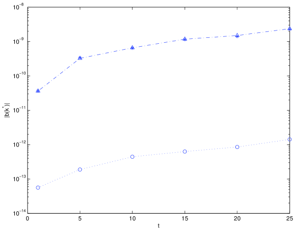
Figure 2: Magnetic field intensity generated by a small intensity velocity source with two different helicities (* and $\triangle$) compared with the nonlinear energy transfer (o)

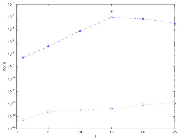
Figure 3: Magnetic field intensity generated by a larger intensity velocity source with two different helicities (* and $\triangle$) compared with the nonlinear energy transfer (o)

In Fig.2 and 3 we show the time evolution of the generated field for the two types of sources as well as the contribution of the nonlinear energy transfer between modes. Each computed point corresponds to the generation of $2\times 10^{6}$ trees. The initial conditions are the same for the computations in the two figures. The only difference is the intensity of the source.

One notices that there is a fast growth of the source-generated field for small times with a subsequent near saturation for the larger source intensity. By contrast the nonlinear energy transfer grows monotonically. One also notices that at these parameter values, the helicity of the source does not seem to have an observable effect.

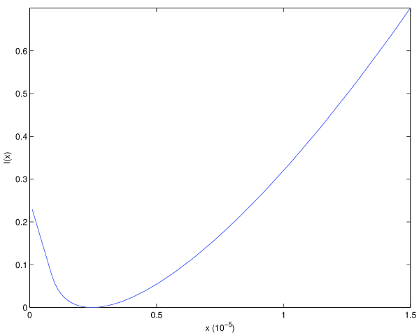
Figure 4: Deviation function for a sample of $2\times 10^{6}$ trees at t=20

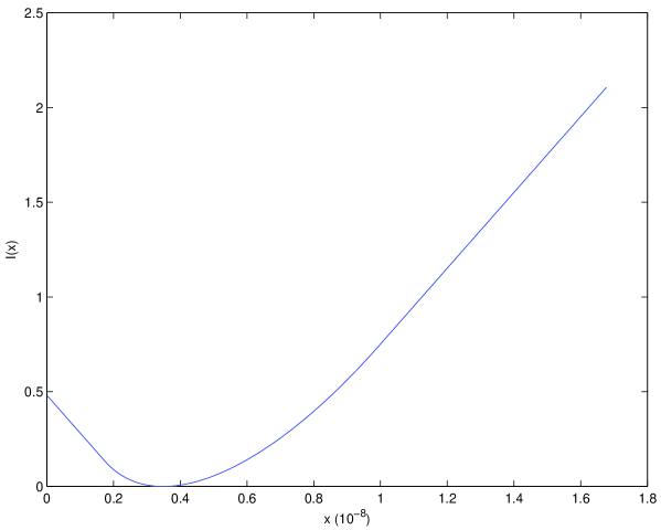
Figure 5: Deviation function for a sample of $2\times 10^{6}$ trees at t=1

The stochastic process that generates the solution has an essentially multiplicative nature. Therefore the reliability of the results should be checked by a large deviation analysis rather than by the standard deviation of the samples. As shown elsewhere [16] the large deviation analysis may be done by the direct construction of the deviation function from the data. First, from the data, one estimates the ”free energy” $c\left(t\right)$

$$c\left(t\right)=\lim_{n\rightarrow\infty}\frac{1}{n}\log E\left\{\exp\left(tW_{n}\right)\right\}$$

$W_{n}$ being the sum of $n$ results. Then one computes the deviation function

$$I\left(x\right)=\sup_{t}\left\{tx-c\left(t\right)\right\}$$

the deviation function giving a logarithmic estimate of the probability $P_{n}$ of a deviation from the sample average

$$P_{n}\left(dx\right)\asymp\exp\left(-nI\left(x\right)\right)dx$$

For our analysis we have taken $40$ samples of $50000$ trees each to approximate the computation of $c\left(t\right)$. The deviation function $I\left(x\right)$ is then computed numerically. In Fig.4 and 5 we have plotted the deviation function for a sample of $2\times 10^{6}$ trees for $t=20$ (Fig.4) and $t=1$ (Fig.5). One notices that the results at $t=20$ are more reliable that at $t=1$, because one sees from the values of $I(x)$ that a larger sample would be needed to obtain the same kind of relative precision.

5 Remarks and conclusions

- Stochastic solutions provide new exact solutions and new numerical algorithms [12] [13] [14]. For the particular case of magnetohydrodynamics, the local phase-space nature of these solutions may be quite appropriate for the studies of plasma turbulence.

- The convergence bounds for the solutions derived in (32) to (38) may be quite small. However one should notice that these bounds are too strict and obtained in a worst case analysis. In practice, by the very nature of the process, the trees finish in finite time (with probability one) and the probability of occurrence of many branches in a tree is rather small. Therefore much larger values of the parameters may be safely used.

- In Section 4 we have exhibited the generation of magnetic fields by a velocity source and the nature of the process has allowed a clear separation of the source effect and the nonlinear transfer of energy between modes. This clear separation of effects is a consequence of the nature of the simulation method and might be profitably used in other contexts.

- An important point to take notice of is the need to have an externally defined stochastic clock in situations of small dissipation. Otherwise nonlinear effects are, in practice, very difficult to study in a reliable manner. This will also be an important point for the practical application of the stochastic solutions for Navier-Stokes [2], [3].

References

- [1] H. P. McKean; Application of brownian motion to the equation of Kolmogorov-Petrovskii-Piskunov, Comm. on Pure and Appl. Math. 28 (1975) 323-331.
- [2] Y. LeJan and A. S. Sznitman; Stochastic cascades and 3-dimensional NavierStokes equations, Prob. Theor. and Rel. Fields 109 (1997) 343-366.
- [3] E. C. Waymire; Probability & incompressible Navier-Stokes equations: An overview of some recent developments, Prob. Surveys 2 (2005) 1-32.
- [4] R. Vilela Mendes and F. Cipriano; A stochastic representation for the Poisson-Vlasov equation, Comm. Nonlinear Sci. and Num. Simul. 13 (2008) 221-226.
- [5] E. Floriani, R. Lima and R. Vilela Mendes; Poisson-Vlasov: stochastic representation and numerical codes, European Physical Journal D 46 (2008) 295-302, 407.
- [6] R. Vilela Mendes; Poisson-Vlasov in a strong magnetic field: A stochastic solution approach, J. Math. Phys. 51 (2010) 043101.
- [7] R. Vilela Mendes; Stochastic solutions of some nonlinear partial differential equations, Stochastics 81 (2009) 279-297.
- [8] R. Vilela Mendes; Poisson-Vlasov in a strong magnetic field: A stochastic solution approach, J. Math. Phys. 51 (2010) 043101.
- [9] F. Cipriano, H. Ouerdiane and R. Vilela Mendes; Stochastic solution of a KPP-type nonlinear fractional differential equation, Fract. Calculus and Appl. Anal. 12 (2009) 47-56.
- [10] E. B. Dynkin; Diffusions, Superdiffusions and Partial Differential Equations, AMS Colloquium Pubs., Providence 2002.
- [11] R. Vilela Mendes; Stochastic solutions of nonlinear pde’s: McKean versus superprocesses, Proc. of CCT11 - Chaos, Complexity and Transport, to appear.
- [12] J. Acebrón, A. Rodriguez-Rozas and R. Spigler; Domain decomposition solution of nonlinear two-dimensional parabolic problems by random trees, J. Comp. Phys. 228 (2009) 5574-5591.
- [13] J.A. Acebrón, A. Rodríguez-Rozas and R. Spigler; Efficient parallel solution of nonlinear parabolic partial differential equations by a probabilistic domain decomposition, J. on Scientific Computing 43 (2010) 135-157.
- [14] J.A. Acebrón and A. Rodríguez-Rozas; A new parallel solver suited for arbitrary semilinear parabolic partial differential equations based on generalized random trees, J. Comp. Phys. 230 (2011) 7891-7909.
- [15] C. Marchioro and M. Pulvirenti; Mathematical theory of incompressible non-viscous fluids, Appl. Math. Sci. vol. 96, Springer-Verlag, New York 1994.
- [16] J. Seixas and R. Vilela Mendes; Large deviation analysis of multiplicity fluctuations, Nuclear Physics B 383 (1992) 622-642.