Galactic Outflows and Evolution of the Interstellar Medium

Abstract

We present a model to self-consistently describe the joint evolution of starburst galaxies and the galactic wind resulting from this evolution. This model will eventually be used to provide a subgrid treatment of galactic outflows in cosmological simulations of galaxy formation and the evolution of the intergalactic medium (IGM). We combine the population synthesis code Starburst99 with a semi-analytical model of galactic outflows and a model for the distribution and abundances of chemical elements inside the outflows. Starting with a galaxy mass, formation redshift, and adopting a particular form for the star formation rate, we describe the evolution of the stellar populations in the galaxy, the evolution of the metallicity and chemical composition of the interstellar medium (ISM), the propagation of the galactic wind, and the metal-enrichment of the intergalactic medium. The model takes into account the full energetics of the supernovae and stellar winds and their impact on the propagation of the galactic wind, the depletion of the ISM by the galactic wind and its impact on the subsequent evolution of the galaxy, as well as the evolving distributions and abundances of metals in the galactic wind. In this paper, we study the properties of the model, by varying the mass of the galaxy, the star formation rate, and the efficiency of star formation. Our main results are the following: (1) For a given star formation efficiency $f_{*}$, a more extended period of active star formation tends to produce a galactic wind that reaches a larger extent. If $f_{*}$ is sufficiently large, the energy deposited by the stars completely expels the ISM. Eventually, the ISM is being replenished by mass loss from supernovae and stellar winds. (2) For galaxies with masses above $10^{11}\mbox{$M_{\odot}$}$, the material ejected in the IGM always falls back onto the galaxy. Hence lower-mass galaxies are the ones responsible for enriching the IGM. (3) Stellar winds play a minor role in the dynamical evolution of the galactic wind, because their energy input is small compared to supernovae. However, they contribute significantly to the chemical composition of the galactic wind. We conclude that the history of the ISM enrichment plays a determinant role in the chemical composition and extent of the galactic wind, and therefore its ability to enrich the IGM.

1 Introduction

Galactic winds and outflows are the primary mechanism by which galaxies deposit energy and metal-enriched gas into the intergalactic medium (IGM). This can greatly affect the evolution of the IGM, and the subsequent formation of other generations of galaxies. Feedback by galactic outflows can provide an explanation for the observed high mass-to-light ratio of dwarf galaxies and the abundance of dwarf galaxies in the Local Group, and can solve various problems with galaxy formation models, such as the overcooling and angular momentum problems (see Benson 2010 and references therein). Galactic outflows can explain the metals observed in the IGM via the Lyman-$\alpha$ forest (e.g. Meyer & York 1987; Schaye et al. 2003; Pieri & Haehnelt 2004; Aguirre et al. 2008; Pieri et al. 2010a, b), the entropy content and scaling relations in X-ray clusters (Kaiser, 1991; Evrard & Henry, 1991; Cavaliere et al., 1997; Tozzi & Norman, 2001; Babul et al., 2002; Voit et al., 2002), and provide observational tests that can constrain theoretical models of galaxy evolution. Local examples of spectacular outflows in dwarf starburst galaxies include those of the extremely metal-poor I Zw 18 (Péquignot 2008; Jamet et al. 2010) and NGC1569 (Westmoquette et al., 2009). More massive spirals, such as NGC7213 (Hameed et al., 2001), also show evidence of global outflows. For a review of the subject, see Veilleux et al. (2005).

1.1 Galactic Outflow Models

Large-scale cosmological simulations have become a major tool in the study of galaxy formation and the evolution of the IGM at cosmological scales. These simulations start at high redshift with a primordial mixture of dark and baryonic matter, and a spectrum of primordial density perturbations. The algorithm simulates the evolution of the system by solving the equations of gravity, hydrodynamics, and (sometimes) radiative transfer. Adding the effect of galactic outflows in these simulations poses a major practical problem. In one hand, the computational volume must be sufficiently large to contain a “fair” sample of the universe, typically several tens of Megaparsecs. On the other hand, the physical processes responsible for generating the outflows take place inside galaxies, at scales of kiloparsecs or less. This represents at the very minimum 4 orders of magnitude in length and 12 orders of magnitude in mass, which is beyond the capability of current computers. Since we cannot simulate both large and small scales simultaneously, the usual solution consists of simulating the larger scales and using a subgrid physics treatment for the smaller scale. Cosmological simulations can predict the location of the galaxies that will produce the outflow, but cannot resolve the inner structure of these galaxies with sufficient resolution to simulate the actual generation of the outflow. Instead, the algorithm will use a prescription to describe the propagation of the outflow and its effect on the surrounding material.

One possible approach consists of depositing momentum or thermal energy “by hand” into the system, to simulate the effect of galactic outflows on the surrounding material (Scannapieco et al., 2001; Theuns et al., 2002; Springel & Hernquist, 2003; Cen et al., 2005; Oppenheimer & Davé, 2006; Kollmeier et al., 2006). The algorithm determines the location of the galaxies producing the outflows and calculates the amount of momentum or thermal energy deposited into the IGM based on the galaxy properties (mass, formation redshift $\ldots$). Then, in particle-based algorithms like smoothed particle hydrodynamics (SPH), this momentum or energy is deposited on the nearby particles, while in grid-based algorithms it is deposited on the neighboring grid points. This will result in the formation and expansion of a cavity around each galaxy, which is properly simulated by the algorithm.

A second approach consists of combining the numerical simulation with an analytical model for the outflows. Tegmark et al. (1993) have developed an analytical model to describe the propagation of galactic outflows in an expanding universe. In this model, a certain amount of energy is released into the interstellar medium (ISM) by supernovae (SNe) during an initial starburst. This energy drives the expansion of a spherical shell that propagates into the surrounding IGM, until it reaches pressure equilibrium. This model, or variations of it, has been used extensively to study the effect of galactic outflows on the IGM (Furlanetto & Loeb 2001; Madau et al. 2001; Scannapieco & Broadhurst 2001; Scannapieco et al. 2002; Scannapieco & Oh 2004; Levine & Gnedin 2005; Pieri et al. 2007, hereafter PMG07; Samui et al. 2008; Germain et al. 2009; Pinsonneault et al. 2010). In this approach, the evolution of the IGM and the propagation of the outflow are calculated separately, but not independently as they can influence one another. The presence of density inhomogeneities in the IGM can affect the propagation of the outflow, while energy and metals carried by the outflow can modify the evolution of the IGM.

There are several limitations with this second approach. In particular, it assumes that the initial starburst, which occurred during the formation of the galaxy, is the only source of energy driving the expansion of the outflow. First, the starburst lasts for a short period of time, typically 50 million years. Hence, we would expect to observe very few galaxies having an outflow. Furthermore these galaxies would be just forming and therefore would have complex and chaotic structures. Observations show instead that outflows are ubiquitous and often originate from well-relaxed galaxies (see Veilleux et al. 2005 and references therein). Second, even though the injection rate of energy is maximum during the initial starburst, the total amount of energy which is injected afterward by all generations of SNe and stellar winds could be comparable or even more important. Even if this energy is injected slowly over a large period of time, the cumulative effect could be significant. Indeed, an initial outflow caused by a starburst could be followed by a steady galactic wind that would last up to the present. The role of stellar winds has been mostly ignored in analytical models and numerical simulations of galactic outflows. Third, there is the possibility that accretion of intergalactic gas onto the galaxy might trigger a second starburst. Finally, a recent study (Sharp & Bland-Hawthorn, 2010) suggests that there is a significant time delay between the initial starburst and the onset of the outflow, something not considered by current models.

Another important issue is the amount of metals contained in the outflow, the spatial distribution of metals in the outflow, and the relative abundances of the various elements. The metallicity of the outflow depends on the metallicity of the ISM at the time of the starburst. The metals contained in the ISM at that time can have several origins: (1) metals already present in the gas when the galaxy formed, (2) the SNe produced during the starburst, and (3) the stellar winds generated by massive stars and AGB objects. Hence, the composition of the outflows will depend on the epoch of formation of the galaxy (which determines the initial metal abundances), as well as the relative amount of metals injected into the ISM by Type Ia SNe, core-collapse SNe (Types Ib, Ic and II), and winds, and the timing of these various processes. As for the amount of metals injected in the IGM, models often assume that it is proportional to the mass of the galaxy, and do not provide a description of the distribution of metals in the outflow and the relative abundances of the elements (Scannapieco & Broadhurst 2001; PMG07).

1.2 Objectives

Our goal is to develop a new galaxy evolution model to improve the treatment of galactic winds in cosmological simulations. This model will describe not only an initial starburst and its resulting outflow, but the entire subsequent evolution of a galaxy up to the present. It will take into account the progressive injection of energy by SNe and stellar winds (which could cause a steady galactic wind that would follow the outflow and last up to the present), and the time-evolution of the metallicity and composition of the ISM that would directly affect the composition of the galactic wind. It will also provide a description of the metal content, metal distribution, and chemical composition of the galactic wind. This emphasis on the structure and composition of the galactic wind is what distinguish our model from recent semi-analytical models of galaxy formation, which tend to focus on reproducing the properties of the galaxies themselves (luminosity and mass functions, halo properties, disk sizes, $\ldots$). For a review of the various semi-analytical models, see Baugh (2006). Our approach combines a population synthesis algorithm to describe the stellar content of the galaxy, an analytical model for the expansion of the galactic wind, and a new model for the distribution of elements inside the galactic wind.

The paper is organized as follows: in §2, we describe the method we use to calculate the mass and chemical composition of stellar winds and SN ejecta, a key ingredient of our algorithm. In §3, we describe the basic equations for the evolution of the ISM. In §4, we describe our galaxy wind model. Results are presented in §5, and conclusions in §6.

2 POPULATION SYNTHESIS MODEL

2.1 Starburst99

Starburst99 (Leitherer et al., 1992; Leitherer & Heckman, 1995; Leitherer et al., 1999; Vázquez & Leitherer, 2005) is the population synthesis code we selected to simulate the properties of the stellar winds and SNe produced by stellar populations with various characteristics. In this project, all simulations use an instantaneous SFR to produce a stellar population of mass $M_{\rm pop}=10^{6}\,\mbox{$M_{\odot}$}$, with a standard IMF as defined by Kroupa (2001). This population is evolved up to a final time $t_{\rm final}=1{\rm Gyr}$, with a timestep $\Delta t=10^{4}{\rm yr}$ (small enough to reproduce each evolutionary phase). The evolutionary tracks are a combination of the Geneva tracks at young ages ($\leq 10^{8}{\rm Myr}$) with the Padova tracks at old ages, to better reproduce the mass loss phases of the massive stars as well as those of smaller-mass objects. We consider four values of the initial metallicity ($Z_{i}=0.001$, 0.004, 0.008, and solar metallicity 0.02). We also specify that all stars with an initial mass $M_{i}$ of 8 to $120\,\mbox{$M_{\odot}$}$ will end as SNe. Binary systems which may also produce SNe are not included in this code and not considered here.

The mass we chose for the stellar population, $M_{\rm pop}=10^{6}\,\mbox{$M_{\odot}$}$, is large enough to provide a good sampling of the IMF. Yet, it is much smaller than the stellar mass of even dwarf galaxies. This enables us to simulate any galaxy SFR we want. To simulate an instantaneous starburst with a stellar mass larger than $M_{\rm pop}$, we simply rescale the results produced by Starburst99. To simulate a SFR that is extended over a finite period of time, we offset the simulations, such that during each timestep $\Delta t$, the correct stellar mass is formed. In §3.1 below, we describe the various SFRs considered in this study.

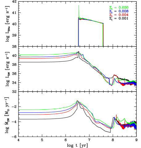
Figure 1: Energy and mass ejected by a single stellar population, versus time. The SNe mechanical energy ($L_{\rm SNe}$, top panel), stellar wind mechanical energy ($L_{\rm SW}$, middle panel), and mass loss rate by stellar winds ($\dot{M}_{\rm SW}$, bottom panel) have been obtained for a $10^{6}\mbox{$M_{\odot}$}$ stellar population, using Starburst99. Different metallicities have been considered as indicated in the top panel.

Starburst99 provides, as a function of time, the mechanical energy produced by SNe and stellar winds, the mass loss by stellar wind, and the chemical composition of the stellar winds, which takes into account the following elements: H, He, C, N, O, Mg, Si, S, and Fe. The code can also predict the mass loss by SNe, but for this project we prefer to use a more detailed treatment which also gives the chemical abundances of the SN yields for a more extensive list of elements. This treatment is described in the next section. Therefore, the ejected mass calculated by Starburst99 will only include the contribution of stellar winds. In Figure 1, we plot the luminosity (rate of mechanical energy injection) associated to SNe, $L_{\rm SNe}$, and stellar winds, $L_{\rm SW}$, and the mass loss by stellar winds, $\dot{M}_{\rm SW}$, versus time, for stellar populations with different metallicities. The initial metallicity has very little effect on the SNe luminosity, but greatly impacts the luminosity and mass loss by stellar winds. This implies that stellar populations that form later will have more powerful winds, since they form out of an ISM that has already been enriched in metals by earlier populations. Figure 1 shows a sudden increase in wind power around 1 - $2\times 10^{6}{\rm yr}$, just prior to the arrival of the first SNe, which is caused by the evolved stages of OB stars, i.e. the Wolf-Rayet stars. The increase in mass loss after $10^{8}{\rm yr}$ is caused by the low-mass stars on the AGB.

2.2 SN Abundances

Except in situations where the metallicity of the stars is larger or equal to solar, the enrichment of the ISM is dominated by SNe (see Fig. 8 of Leitherer et al. 1992). Thus, it is important to know the composition of the material ejected by SNe as a function of the initial mass and metallicity of the stellar progenitors. Several groups have used models of stellar evolution and nucleosynthesis to produce tables of chemical abundances for SN ejecta. These studies are summarized in Table 1. The first column gives the authors of the papers; the second and third columns list the metallicities and initial masses considered, respectively; the fourth column indicates whether or not mass loss prior to the SN explosion was included in the model.

Table 1: SN yields available in the literature.

Paper	$Z$	$M_{i}\>[\mbox{$M_{\odot}$}]$	$\dot{M}$
Woosley & Weaver (1995)	0, $2\times 10^{-6}$, $2\times 10^{-4}$, 0.002, 0.02	11, 12, 13, 15, 18, 19, 20, 25, 30, 35, 40	no
Chieffi & Limongi (2004)	0, $10^{-6}$, $10^{-4}$, 0.001, 0.006, 0.02	13, 15, 20, 25, 30, 35	no
Nomoto et al. (2006)	0, 0.001, 0.004, 0.02	13, 15, 18, 20, 25, 30, 35, 40	yes
Woosley & Heger (2007)	0.02	32 $M_{i}$’s between 12 and 120	yes
Limongi & Chieffi (2007)	0.02	15 $M_{i}$’s between 10 and 120	yes
Heger & Woosley (2010)	0	120 $M_{i}$’s between 10 and 100	no

Although very useful, these studies are not fully satisfactory for our work. The first three studies (Woosley & Weaver 1995; Chieffi & Limongi 2004; Nomoto et al. 2006, hereafter N06) consider a wide range of metallicities, from no metallicity ($Z=0$) to solar metallicity ($Z_{\odot}=0.02$), but are limited to initial masses $M_{i}\leq 40\,\mbox{$M_{\odot}$}$. The next three studies (Woosley & Heger 2007, hereafter WH07; Limongi & Chieffi 2007; Heger & Woosley 2010, hereafter HW10) consider initial masses up to 100 - $120\,\mbox{$M_{\odot}$}$, but only one value of the metallicity. Also, three of these studies do not include mass loss prior to the explosion, which is critical in our models since we include stellar wind effects. The study that comes the closest to our needs is the one of N06. This is the only study that covers metallicities in the range $Z=0$ - $Z_{\odot}$ and includes mass loss. However, its mass range only goes from 13 to $40\,\mbox{$M_{\odot}$}$. These tables need to be extrapolated both at the low-mass and high-mass end to cover the full range of SNe progenitor masses. In this paper, we assume an IMF with lower and upper mass limits of $1$ and $120\,\mbox{$M_{\odot}$}$, respectively, and SNe progenitor masses in the range $M_{i}=8$ - $120\,\mbox{$M_{\odot}$}$. The lower limit of $8\mbox{$M_{\odot}$}$ is the most commonly used, but that value is actually quite uncertain, and could have an important effect on the results (see Fig. 5 below).

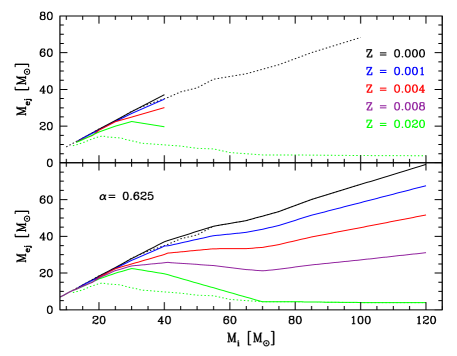
Figure 2: Top panel: Total mass ejected by one SN versus the initial mass of the progenitor, according to the tables of N06 (solid lines), WH07 (lower dotted line), and HW10 (upper dotted line). Colors represent various metallicities, as indicated. Bottom panel: Total mass ejected by one SN versus the initial mass of the progenitor after extrapolating down to $M_{i}=8\,\mbox{$M_{\odot}$}$ and up to $M_{i}=120\,\mbox{$M_{\odot}$}$, for metallicities $Z=0$ (solid black line) and $Z=Z_{\odot}$ (solid green line), after extrapolating over all metallicities available in N06 (blue and red lines), and after interpolating to the metallicity $Z=0.008$ used by Starburst99 (purple line).

The top panel of Figure 2 shows the mass ejected by SNe versus initial mass and metallicity, calculated with the tables of N06 (solid curves). An interesting feature is the linear relation between $M_{\rm ej}$ and $M_{i}$ at $Z=0$. Also, all the curves converge together at $M_{i}=13\,\mbox{$M_{\odot}$}$, suggesting that for initial masses $M_{i}<13\,\mbox{$M_{\odot}$}$, the ejected mass is independent of metallicity. To extrapolate down to $M_{i}=8\,\mbox{$M_{\odot}$}$, we used the composition for $M_{i}=13\,\mbox{$M_{\odot}$}$, modulated using the linear regression at $Z=0$ calculated with the software Slope (Isobe et al., 1990). The result is also shown in Figure 2.

Extrapolation up to $120\,\mbox{$M_{\odot}$}$ can be tricky, especially if mass loss is considered. Several approaches have been suggested in the literature, especially at the high-mass end. Martinez-Serrano et al. (2008) extrapolate the mass ejected $M_{\rm ej}$ and chemical composition of the ejecta linearly up to $M_{i}=100\,\mbox{$M_{\odot}$}$. Oppenheimer & Davé (2008) assume similar ejecta for stars in the range $M_{i}=35$ - $100\,\mbox{$M_{\odot}$}$ and also for stars in the range $M_{i}=10$ - $13\,\mbox{$M_{\odot}$}$. Tornatore et al. (2007) and Scannapieco et al. (2005) assume that stars with initial masses larger than $40\,\mbox{$M_{\odot}$}$ end up directly in a black hole, with no ejecta. Using linear interpolation up to $M_{i}=120\,\mbox{$M_{\odot}$}$ would be risky. The relation between $M_{\rm ej}$ and $M_{i}$ becomes metallicity-dependent for $M_{i}>25$ - $30\,\mbox{$M_{\odot}$}$, implying that only two or three points would be available to extrapolate over a mass interval three times wider than the one of N06. Furthermore at $Z=Z_{\odot}$, $M_{\rm ej}$ eventually decreases with increasing initial mass and a linear extrapolation would eventually lead negative values before reaching $M_{i}=120\,\mbox{$M_{\odot}$}$. Setting the ejected mass to zero for $M_{i}>40\,\mbox{$M_{\odot}$}$ is not a good solution either. Even if the SN results in the formation of a black hole, that black hole is never as massive as the progenitor (Woosley et al. 2002; WH07; Limongi & Chieffi 2008; Zhan et al. 2008; Belczynski et al. 2010). Using a copy of the $M=40\,\mbox{$M_{\odot}$}$ at larger masses is not realistic either since the tendency clearly shows that there is more material ejected for larger initial masses, except at $Z_{\odot}$.

Since none of the three extrapolation methods considered so far is satisfactory for extrapolating up to $120\,\mbox{$M_{\odot}$}$, we developed an alternative method. We started by extrapolating the table of N06 at $Z=0$ and also $Z_{\odot}$, by combining them with the tables of HW10 and WH07, respectively. The top panel of Figure 2 shows the $Z_{\odot}$ relation of WH07 and the $Z=0$ relation of HW10 (dotted curves). The $Z=Z_{\odot}$ relations of N06 and WH07 differ significantly in the range $M_{i}=20$ - $40\,\mbox{$M_{\odot}$}$. This is likely the consequence of using a different prescription for the mass loss during the pre-SN phase. In the model of WH07, the ejected mass reaches a maximum around $M_{i}=21\,\mbox{$M_{\odot}$}$, then decreases with increasing initial mass, and finally reaches a plateau at $M_{\rm ej}=4\,\mbox{$M_{\odot}$}$, which represents the minimum mass a SN can eject. Assuming that this limit is correct, we extrapolated the $Z_{\odot}$ model of N06 until it reaches the model of WH07 (around $M_{i}=70\,\mbox{$M_{\odot}$}$). We then switched to the model of WH07 to complete the extrapolation up to $M_{i}=120\,\mbox{$M_{\odot}$}$. For $Z=0$, the results of N06 and HW10 are essentially identical in the range $M_{i}=13$ - $30\,\mbox{$M_{\odot}$}$, and very similar in the range $M_{i}=30$ - $40\mbox{$M_{\odot}$}$. To combine them, we used the tables of N06 in the range $M_{i}=8$ - $40\,\mbox{$M_{\odot}$}$ and the tables of HW10 in the range $M_{i}=55$ - $120\,\mbox{$M_{\odot}$}$, Between 40 and $55\,\mbox{$M_{\odot}$}$, we interpolated between these two masses. The results are shown in the bottom panel of Figure 2.

At the two intermediate metallicities $Z=0.001$ and 0.004, the values of the ejected masses should lie between the values for $Z=0$ and $Z_{\odot}$ (Fig. 2). If the mass loss due to stellar winds were neglected, the masses ejected by SNe should be the same as for models with $Z=0$. The mass loss associated with massive stars is proportional to $Z^{\alpha}$, where $\alpha\simeq 0.6$ - 0.8 (Vink et al., 2001; Vink & de Koter, 2005; Krticka, 2006; Mokiem et al., 2007). We then interpolated to get the mass ejected by SNe at any metallicity:

$$M_{\rm ej}(M_{i},Z)=M_{\rm ej}(M_{i},0)-\tau(M_{i},Z)\dot{M}\,,\quad\dot{M}=AZ^{\alpha}\,,$$ (1)

where $A$ is a constant, and $\tau(M_{i},Z)$ is the lifetime of a star of initial mass $M_{i}$ and metallicity $Z$. We made the approximation that the lifetime does not vary much with metallicity, $\tau(M_{i},Z)\approx\tau(M_{i})$. Equation (1) becomes:

$$M_{\rm ej}(M_{i},Z)=M_{\rm ej}(M_{i},0)-B(M_{i})Z^{\alpha}\,.$$ (2)

where the function $B(M_{i})$ was calculated from the masses ejected at $Z=Z_{\odot}$:

$$B(M_{i})={M_{\rm ej}(M_{i},Z_{\odot})-M_{\rm ej}(M_{i},0)\over Z_{\odot}^{\alpha}}\,.$$ (3)

We choose the value $\alpha=0.625$, which minimizes the discontinuity at $M=40\,\mbox{$M_{\odot}$}$. Figure 2 shows all the models of N06 after extrapolation. For $Z=0.004$ and 0.001, the mass loss is not as extreme as in the case $Z=Z_{\odot}$. For that reason, we used the composition of the $40\,\mbox{$M_{\odot}$}$ models modulated according to the value of $M_{\rm ej}$ for all the initial masses $M_{i}>40\,\mbox{$M_{\odot}$}$.

Next we determined the composition of the ejected masses, for $Z=0$ and $Z_{\odot}$. Table 2 shows the hydrogen mass, helium mass, and total mass ejected for the WH07 models. The cases presented are extreme. The mass loss by stellar winds is sufficiently large to expel the entire hydrogen envelop and most of the helium as well. This indicates that these stars have evolved through a Wolf-Rayet stage, resulting in SNe of Type Ib or Ic. Hence, most of the material ejected is composed of metals. For this reason, we treated hydrogen and helium as we treated the total mass ejected: we followed the tables of N06 until it reaches the model of WH07 and then switched to the model of WH07 (Fig. 3). The reminder of the ejected mass was assumed to have the chemical composition corresponding to the $M_{i}=40\,\mbox{$M_{\odot}$}$ model. For $Z=0$, the complete composition of the $M_{i}=40\,\mbox{$M_{\odot}$}$ model was used.

Table 2: Hydrogen mass, helium mass, and total mass ejected by SNe versus initial mass at solar metallicity, according to the table of WH07.

$M_{i}[\mbox{$M_{\odot}$}]$	$M_{\rm H}[\mbox{$M_{\odot}$}]$	$M_{\rm He}[\mbox{$M_{\odot}$}]$	$M_{\rm ej}[\mbox{$M_{\odot}$}]$
40	0.223	1.640	9.74
50	$5.51\times 10^{-8}$	0.068	7.94
60	$1.77\times 10^{-7}$	0.120	5.65
70	$1.16\times 10^{-7}$	0.152	4.35
80	$1.04\times 10^{-7}$	0.156	4.34
100	$1.77\times 10^{-7}$	0.181	3.96
120	$1.39\times 10^{-7}$	0.172	3.92

Starburst99 requires tables of SNe at metallicities $Z=0.001$, 0.004, 0.008, and 0.02. At this point we have tables at $Z=0.004$ and $0.02$. For $Z=0.008$, we interpolated between the tables at $Z=0.004$ and 0.02 using $\log Z$ as an interpolation variable. We now have a full set of SN tables that provides the ejected mass and composition of the ejecta, for all progenitors in the range $M_{i}=8$ - $120\,\mbox{$M_{\odot}$}$ and $Z=0$ - $Z_{\odot}$. Figure 2 shows the ejected mass versus progenitor mass.

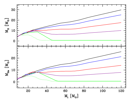
Figure 3: Hydrogen (top) and helium mass (bottom) ejected by one SN versus the initial mass of the progenitor, according to the tables of N06 (solid lines), after extrapolating down to $M_{i}=8\mbox{$M_{\odot}$}$ and up to $M_{i}=120\mbox{$M_{\odot}$}$, for $Z=Z_{\odot}$. The dotted line illustrates the $Z=Z_{\odot}$ model of WH07. Colors have the same meaning as in Figure 2.

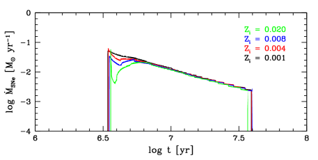
Figure 4: Mass loss rate by SNe versus time. Number of stars and SN explosions are from a Starburst99 model for an instantaneous burst with a standard IMF and a total mass of $10^{6}\mbox{$M_{\odot}$}$. Mass ejected by each SN comes from our extended tables. Different metallicities have been considered as indicated.

Figure 5: Mass ejected by SNe versus metallicity, Top panel: results obtained with our extrapolation method for the SN mass ejected as a function of the progenitor initial mass, using the same stellar population model as in Figure 4 (dotted curve), compared with results obtained with different extrapolation methods (solid curves): from top to bottom: linear extrapolation of Martinez-Serrano et al. (2008), constant approximation of Oppenheimer & Davé (2008), and no-ejecta approximation of Tornatore et al. (2007) and Scannapieco et al. (2005). Bottom panel results obtained with our extrapolation method, for various values of the minimum initial mass. From top to bottom, $M_{i}=6\mbox{$M_{\odot}$}$, $8\mbox{$M_{\odot}$}$, and $10\mbox{$M_{\odot}$}$.

At each timestep during the simulation, Starburst99 provides the number of SNe and their luminosity (adopting that each SN produces $10^{51}{\rm ergs}$; McKee 1990). The SN tables are then used to calculate at every timestep the mass and composition of the material deposited into the ISM. For simulations with initial metallicity $Z=0$, we use the luminosity at $Z=0.001$ which is the smallest value considered by Starburst99. Figure 4 shows the mass loss rate due to SNe for a $10^{6}\,\mbox{$M_{\odot}$}$ instantaneous burst. This completes the results shown in Figure 1. In the top panel of Figure 5, we plot the total mass ejected by SNe versus metallicity, for the same population. The dotted curve shows our extrapolation method, while the solid curves show the three other methods. The “constant” method of Oppenheimer & Davé (2008) (using the ejecta for $M_{i}=40\mbox{$M_{\odot}$}$ at higher masses) is the one which resembles our method the most, but there are significant differences. This justifies a posteriori the method we have developed in this section.

We assume a minimum progenitor mass of $M_{i}=8\mbox{$M_{\odot}$}$, but we also generated other tables using different values. The bottom panel of Figure 5 shows the ejected mass for minimum progenitor masses of $M_{i}=6\mbox{$M_{\odot}$}$, $M_{i}=8\mbox{$M_{\odot}$}$ (the value assumed in this paper), and $M_{i}=10\mbox{$M_{\odot}$}$. The differences are of order 50%, with the ejected mass being larger for a smaller minimum progenitor mass. This shows that the particular choice of minimum progenitor mass can have a impact on the results, and we intend to investigate this issue in more details in future work. Here we focus on the case of a minimum progenitor mass of $M_{i}=8\mbox{$M_{\odot}$}$.

In a recent paper, Horiuchi et al. (2011) point to a serious “supernova rate problem”: the measured cosmic massive-star formation rate predicts a rate of core-collapse supernovae about twice as large as the observed rate, at least for redshifts between 0 and 1, where surveys are thought to be quite complete. Several explanations are proposed to explain this major discrepancy, including a large fraction of unusually faint (intrinsically or dust-attenuated), and thus unaccounted for, core-collapse SNe and a possible overestimate of the star formation rate based on the current estimators. If indeed this supernova rate problem is real, the SFR (see §5.1) might have to be scaled accordingly. However, all simulations presented in this paper start at redshift $z=15$, and terminate at redshifts between 6 and 9. It is not clear that there is a supernova rate problem at these redshifts.

3 EVOLUTION OF THE INTERSTELLAR MEDIUM

During the evolution of a galaxy, the ISM is constantly enriched by ejecta from stellar winds and SNe. Hence, every generation of stars provides an environment richer in metals for the future generations. The level of this enrichment depends on the SFR, since the metal production increases with the number of stars formed. To simulate this process, we designed an algorithm that combines the outputs of Starburst99 with the SNe tables of N06.

3.1 Initial Conditions

We consider a galaxy with a total mass $M_{\rm gal}$. We assume that the ratio of baryons to dark matter in the galaxy is equal to the universal ratio, which is a valid assumption for the initial stages of the galaxy. The baryonic mass of the galaxy is then given by

$$M_{b}={\Omega_{b0}\over\Omega_{0}}M_{\rm gal}\,,$$ (4)

where $\Omega_{0}$ and $\Omega_{b0}$ are the total and baryon density parameters, respectively. We assume that each galaxy starts up with a primordial composition of hydrogen and helium ($X=0.755$ and $Y=0.245$). The formation of the galaxy results in a starburst, during which a fraction $f_{*}$ of the baryonic mass is converted into stars. The total mass in stars at the end of the starburst is therefore

$$M_{*}=f_{*}M_{b}\,.$$ (5)

We refer to the parameter $f_{*}$ as the star formation efficiency.

We consider three different types of star formation rate: instantaneous, constant, and exponential. With an instantaneous SFR, all stars form at $t=0$. In the other cases, the stellar mass formed $M_{*}$ and the star formation rate $\dot{M}_{*}$ are related by

$$\int_{0}^{t_{f}}\dot{M}_{*}(t)dt=M_{*}\,,$$ (6)

where $t_{f}$ is the final time of the simulation. For a constant SFR, we have

$$\dot{M}_{*}={M_{*}\over t_{\rm burst}}\,,$$ (7)

where $t_{\rm burst}$ is the duration of the starburst. We usually choose a value for $\dot{M}_{*}$ and solve equation (7) for $t_{\rm burst}$. For an exponential SFR, we have

$$\dot{M}_{*}={M_{*}\over t_{c}}e^{-t/t_{c}}\,,$$ (8)

where $t_{c}=5\times 10^{7}{\rm yrs}$ is the characteristic time. Since star formation never ends in this case, the stellar mass formed depends on the final time $t_{f}$. Equation (8) is valid in the limit $t_{f}\gg t_{c}$.

There are some caveats about equations (4) and (5). The infalling gas must cool and form molecular clouds which then fragment into stars. If star formation is delayed until all the gas has cooled, then equation (4) would be valid, but it is more likely that star formation will start while a fraction of the gas has not cooled yet. SNe and stellar winds from that first generation of stars will inhibit the formation of subsequent generations of stars, by reheating the ISM and possibly expelling some of it in the form of a galactic outflow. Observations of galaxies in the redshift range $0<z<4$ show that star formation is a very inefficient process, with $M_{*}/M_{\rm gal}<0.03$ (Behroozi et al., 2010). Hence, the value of $M_{b}$ in equation (4) is an upper limit, which does not take into account the gas lost by galactic outflows. As for the reheating of the gas and suppression of inflow, it is implicitly taken into account in equation (5) by introducing a star formation efficiency $f_{*}$. The mass of gas that was reheated and prevented from forming stars is $M_{\rm reheat}=(1-f_{*})M_{b}$. In this paper, we consider star formation efficiencies $f_{*}=0.1$, 0.2, 0.5, and 1.0. Equations (4) and (5) then give $M_{*}/M_{\rm gal}=0.016$, 0.032, 0.081 and 0.162, respectively. The first two values are consistent with observations. The last two values are quite extreme, and we considered them mostly to investigate the behavior of the model under extreme conditions.

In this paper, we impose various forms for the SFR to investigate the effect of the SFR on the properties of the galactic outflows. The effect of feedback and reheating of the ISM is all contained implicitly in the value of $f_{*}$. To provide a proper treatment of the aforementioned feedback processes, we intend to modify the model such that the SFR will be recalculated at every time step, from the physical conditions of the ISM gas at that time, taking into account the effect of all previous generation of stars. This will provide a consistent treatment of feedback and self-regulating star formation, and eliminate the need to specify a priori a star formation efficiency $f_{*}$. This will be the subject of a forthcoming paper.

3.2 Evolution of the Mass and Composition of the ISM

Our algorithm tracks the evolution of $M_{\rm ISM_{X}}$, the mass of element X contained in the ISM. At the beginning of each timestep, the total mass of the ISM is given by

$$M_{\rm ISM}(t)=\sum_{\rm X}M_{\rm ISM_{X}}(t)\,,$$ (9)

where the sum is over all elements included in the algorithm, that is all elements from hydrogen (${\rm X}=1$) to gallium (${\rm X}=31$). These quantities are initialized at the beginning of the simulation, and updated during each timestep $\Delta t$, as follows. First, we calculate the mass ejected by stellar winds and SNe. We include the contribution from all stars present at that time, taking into account their current ages, initial metallicities, and initial masses:

$$M_{\rm SW_{X}}(t) = \sum_{k}\dot{M}_{\rm SW_{X}}^{\rm SB99}(\tau_{k},Z_{k},M_{k})\Delta t\,,$$ (10)

$$M_{\rm SNe_{X}}(t) = \sum_{k}\dot{M}_{\rm SNe_{X}}^{\rm SB99}(\tau_{k},Z_{k},M_{k})\Delta t\,.$$ (11)

where $\tau_{k}$, $Z_{k}$, and $M_{k}$ are the current age, initial metallicity, and mass of population $k$, respectively. The sums are over all the stellar populations that have already formed by time $t$. The superscript SB99 indicates quantities calculated by Starburst99. We also calculate the total luminosity produced by SNe and stellar winds:

$$L_{\rm SW}(t) = \sum_{k}L_{\rm SW}^{\rm SB99}(\tau_{k},Z_{k},M_{k})\,,$$ (12)

$$L_{\rm SNe}(t) = \sum_{k}L_{\rm SNe}^{\rm SB99}(\tau_{k},Z_{k},M_{k})\,.$$ (13)

We then remove from the ISM the total mass of the stars born during that timestep, and the mass removed by the galactic wind, and add the material ejected by SNe and stellar winds:

$$M_{\rm ISM_{X}}(t+\Delta t)=M_{\rm ISM_{X}}(t)-{M_{\rm ISM_{X}}(t)\over M_{\rm ISM}(t)}\big{[}\dot{M}_{*}(t)$$

$$\qquad+\dot{M}_{\rm GW}(t)\big{]}\Delta t+M_{\rm SW_{X}}(t)+M_{\rm SNe_{X}}(t)\,,$$ (14)

where $\dot{M}_{\rm GW}(t)$ is the rate of mass loss by galactic wind (the calculation of $\dot{M}_{\rm GW}$ is presented in the next section). The mass remove from the ISM by the star formation process is used to generate several new stellar populations. Each population is given an initial mass $M_{k}$, an initial metallicity $Z_{k}$ equal to the metallicity $Z(t)$ of the ISM at that time, and we set the age $\tau_{k}$ of these new populations to zero. We then recompute the ISM metallicity:

$$Z(t+\Delta t) = \Big{[}M_{\rm ISM}(t+\Delta t)-M_{\rm ISM_{H}}(t+\Delta t)$$ (15)

$$-M_{\rm ISM_{He}}(t+\Delta t)\Big{]}\Big{/}M_{\rm ISM}(t+\Delta t)\,.$$

This expression accounts for the material removed from the ISM by the star formation process and the galactic wind, and it also considers the enriched material added by stars already formed. Finally, we update the age of every stellar population:

$$\tau_{k}(t+\Delta t)=\tau_{k}(t)+\Delta t\,,\qquad\hbox{for all }k\,.$$ (16)

These operations are repeated at every timestep in the simulation.

In our model, $M_{\rm ISM_{X}}$ is a function of time only. This assumes that metals ejected into the ISM by SNe and stellar winds are instantaneously mixed. This commonly-used approximation has the advantage of being simple to implement. However, in reality, it will take some finite time before the metals are fully mixed. For this reason, the efficiency of metal-enrichment of the IGM in our model should be considered as an upper limit.

Starburst99 cannot calculate directly the mass loss and luminosities appearing in equations (10) to (13) for any initial metallicity $Z_{i}$. It is limited to the values $Z_{i}=0.001$, 0.004, 0.008, and 0.02. We therefore need to interpolate the results of Starburst99 in order to get the quantities $\dot{M}^{\rm SB99}$ and $L^{\rm SB99}$. For values of $Z_{i}$ in the range $[0.001,0.02]$, we calculate $\dot{M}^{\rm SB99}$ and $L^{\rm SB99}$ at the metallicities immediately before and after $Z_{i}$, and interpolate between them, using equations of the form

$$\log\dot{M}^{\rm SB99} = A\log Z_{i}+B\,,$$ (17)

$$\log L^{\rm SB99} = C\log Z_{i}+D\,.$$ (18)

In the range $[0,0.001]$, we treat stellar winds and SNe differently. We assume that, in that range, the mass loss by stellar wind is proportional to $Z_{i}^{\alpha}$, with $\alpha\approx 0.625$, as in equations (1) to (3). Hence,

$$\dot{M}_{\rm SW}^{\rm SB99}(Z_{i}) = \dot{M}_{\rm SW}^{\rm SB99}(0.001)\left({Z_{i}\over 0.001}\right)^{0.625}\,,$$ (19)

$$L_{\rm SW}^{\rm SB99}(Z_{i}) = L_{\rm SW}^{\rm SB99}(0.001)\left({Z_{i}\over 0.001}\right)^{0.625}\,.$$ (20)

For SNe, we use the values $L_{\rm SNe}^{\rm SB99}(Z_{i}=0.001)$ at lower metallicities. This is a valid approximation because the dependence of the stellar lifetimes on metallicity is weak, as Figure 1 shows.

3.3 Mass Loss by Galactic Wind

The presence of a galactic wind enables a fraction of the ISM to escape the galaxy and enrich the surrounding IGM. Since the wind is generated by the thermal energy deposited in the ISM by stars, we expect the mechanical energy of the galactic wind to be proportional to the rate of energy injection by SNe and stellar winds:

$${1\over 2}\dot{M}_{\rm GW}(t)V_{\rm GW}^{2}\propto L(t)\,,$$ (21)

where $\dot{M}_{\rm GW}$ and $V_{\rm GW}$ are the mass loss rate by galactic wind and the velocity of the wind, respectively. The galactic wind will create a cavity expanding into the IGM (see § 4 below). The expansion of the cavity is driven by the mechanical energy $\dot{M}_{\rm GW}(t)V_{\rm GW}^{2}/2$ deposited into the IGM by the wind, but does not depend separately on $\dot{M}_{\rm GW}$ and $V_{\rm GW}$. Hence, to determine $\dot{M}_{\rm GW}$, we must make an additional assumption. There are two limiting cases: One limit consists of having $\dot{M}_{\rm GW}$ constant, in which case increasing the number of SNe will increase the wind velocity. The opposite limit consists of having a constant wind velocity $V_{\rm GW}$, in which case an increase in the number of SNe results in a larger amount of matter being ejected.

It would take detailed high-resolution simulations to determine which of these limits is correct. Ultimately, the critical factor should be the spatial distribution of SNe. A single SN will only affect the ISM located in its vicinity. In the case of several SNe, there collective effect should critically depend on their level of clustering. If all SNe are concentrated in a same location, the same region will be affected, and the net effect will be to eject the same matter, but at a larger velocity. If instead the SNe are distributed throughout the galaxy, each SN will affect a different part of the ISM, and the net result will be to eject more material, but at the same velocity. This last case is the limit we adopt in this paper. Consequently, the reader should keep in mind that our estimates of the amount of material ejected is an upper limit. Under this assumption the rate of mass loss by the galactic wind is proportional to the luminosity,

$$\dot{M}_{\rm GW}(t)\propto L(t)\,,$$ (22)

To determine the constant of proportionality, we first integrate the functions $\dot{M}_{\rm GW}(t)$ and $L(t)$ over the lifetime of the galaxy:

$$M_{\rm GW}^{\rm tot} = \int_{0}^{t_{f}}\dot{M}_{\rm GW}\,dt\,,$$ (23)

$$E^{\rm tot} = \int_{0}^{t_{f}}L\,dt\,,$$ (24)

where $M_{\rm GW}^{\rm tot}$ is the total mass ejected into the galactic wind, and $E^{\rm tot}$ is the total energy deposited in the ISM. We can rewrite equation (22) as

$$\dot{M}_{\rm GW}(t)={M_{\rm GW}^{\rm tot}\over E^{\rm tot}}L(t)\,.$$ (25)

The problem is that $M_{\rm GW}^{\rm tot}$ and $E^{\rm tot}$ are not known until the simulation is completed, and to perform the simulation, we need to know these quantities in advance in order to calculate $\dot{M}_{\rm GW}$ at every timestep. To solve this problem, we replace $M_{\rm GW}^{\rm tot}$ and $E^{\rm tot}$ in equation (25) by approximations that can be calculated ab initio, before actually performing the simulation.

3.3.1 Estimate of $E^{\rm tot}$.

The luminosity $L(t)$ is calculated as the simulation proceeds, but we can estimate it as follows: first, as we shall see below, the contribution of stellar winds to the luminosity becomes negligible once the SNe phase starts. If we neglect stellar winds, and also neglect the weak dependence of the SN luminosity on the metallicity (see Fig. 1), we can directly estimate the luminosity from the star formation rate $\dot{M}_{*}$. We define an integrated mass loss rate $\dot{F}(t)$ using:

$$\dot{F}(t+t_{\rm onset})\equiv\int_{t-t_{\rm active}}^{t}\dot{M}_{*}(t^{\prime})dt^{\prime}\,,$$ (26)

where $t_{\rm onset}$ is the time elapsed between the formation of the stellar population and the onset of the first SN, and $t_{\rm active}$ is the time duration of the SNe phase. Figure 6 shows the luminosity $L(t)$ obtain from the simulation, and the quantity $\dot{F}(t)$ calculated using $t_{\rm onset}=3.11\,{\rm Myr}$ and $t_{\rm active}=39.2\,{\rm Myr}$ (Fig. 1). To a very good approximation, $\dot{F}(t)$ is proportional to $L(t)$. We can therefore approximate equation (25) as

$$\dot{M}_{\rm GW}={M_{\rm GW}^{\rm tot}\over F^{\rm tot}}\dot{F}(t)\,,$$ (27)

where

$$F^{\rm tot}=\int_{0}^{t_{f}}\dot{F}\,dt\,.$$ (28)

Figure 6: Solid curve: SNe luminosity versus time, for a $10^{9}\mbox{$M_{\odot}$}$ galaxy with an exponential SFR and a star formation efficiency $f_{*}=0.1$. Dotted curve: Integrated mass loss rate $\dot{F}(t)$, for the same galaxy.

Both $\dot{F}(t)$ and $F^{\rm tot}$ are calculated at the beginning of the simulation.

3.3.2 Estimate of $M_{\rm GW}^{\rm tot}$.

We still need to determine the total mass ejected by the galactic wind, $M_{\rm GW}^{\rm tot}$, to be able to use equation (27). Like the total energy deposited in the ISM, $E^{\rm tot}$, $M_{\rm GW}^{\rm tot}$ is not known until the simulation is completed. To estimate it, we replace $\dot{M}_{\rm GW}$ in equation (23) by an approximation that can be calculated at the beginning of the simulation. We then integrate to get $M_{\rm GW}^{\rm tot}$, we substitute that value in equation (27), which then provides the mass loss by galactic wind during the simulation. To find an initial approximation for $\dot{M}_{\rm GW}$, we first notice that observations at different redshifts suggest a relation between the mass loss by galactic winds and the star formation rate (Martin, 1999), often expressed in terms of the ratio

$$\eta\equiv{\dot{M}_{\rm GW}\over\dot{M}_{*}}\,.$$ (29)

This value appears to vary significantly among galaxies, with values ranging from 0.01 to 10 (Veilleux et al., 2005). Murray et al. (2005) derived analytical relations between the factor $\eta$ and the velocity dispersion $\sigma$, for both momentum-driven and energy-driven winds. We focus in this paper on energy-driven winds, but will consider momentum-driven winds in future work. For energy-driven winds, Murray et al. (2005) derived the following relation:

$$\dot{M}_{\rm GW}=\dot{M}_{*}\,\xi_{0.1}\,\varepsilon_{3}^{\phantom{1}}\left({300\,{\rm km\,s^{-1}}\over\sigma}\right)^{2}\,,$$ (30)

where $\sigma$ is the velocity dispersion, $\varepsilon_{3}^{\phantom{1}}\equiv 1000E^{\rm tot}/M_{*}c^{2}$, and $\xi_{0.1}\equiv f_{w}/0.1$, with $f_{w}(M_{\rm gal})$ the fraction of energy provided by stars that is used to power the wind, for a galaxy of mass $M_{\rm gal}$ (Scannapieco et al., 2002). To calculate $\varepsilon_{3}^{\phantom{1}}$, we use Starburst99 with a $10^{6}\mbox{$M_{\odot}$}$ stellar population and a standard IMF. The total energy $E^{\rm tot}$ produced by SNe and stellar winds is always of the order of $10^{55.3}{\rm ergs}$, for all metallicities. This gives $\varepsilon_{3}^{\phantom{1}}=0.011$. Equation (30) reduces to

$$\dot{M}_{\rm GW}=0.11\dot{M}_{*}f_{w}\left({300\,{\rm km\,s^{-1}}\over\sigma}\right)^{2}\,.$$ (31)

For a galaxy of mass $M_{\rm gal}$, the velocity dispersion $\sigma$ is calculated using the equation of Oppenheimer & Davé (2008):

$$\sigma=200\left[{M_{\rm gal}\over 5\times 10^{12}\mbox{$M_{\odot}$}}h{H(z_{\rm gf})\over H_{0}}\right]^{1/3}{\rm km\,s^{-1}}\,,$$ (32)

where $z_{\rm gf}$ is the formation redshift of the galaxy, $H$ is the Hubble parameter, with $H_{0}$ being its present value, and $h=H_{0}/100\,\rm km\,s^{-1}\,Mpc^{-1}$. Equations (31) and (32) give us an estimate of $\dot{M}_{\rm GW}$. We then apply equation (23) to calculate $M_{\rm GW}^{\rm tot}$, which we substitute in equation (27). This equation is then used to calculate the mass loss by galactic wind during the simulation [eq. (3.2)].

Figure 7: Escape fraction versus redshift, for a $10^{9}\mbox{$M_{\odot}$}$ galaxy with a star formation efficiency $f_{*}=0.1$.

The parameter $f_{\rm esc}$ is defined as the fraction of the ISM mass that escapes the galaxy:

$$f_{\rm esc}={M_{\rm GW}^{\rm tot}\over M_{b}}={\Omega_{0}\over\Omega_{b0}}{M_{\rm GW}^{\rm tot}\over M_{\rm gal}}\,.$$ (33)

Figure 7 shows $f_{\rm esc}$ versus formation redshift $z_{\rm gf}$, for various galactic masses $M_{\rm gal}$, with a star formation efficiency of $f_{*}=0.1$. The dependence on $z_{\rm gf}$ comes entirely from the factor $H(z_{\rm gf})$ in equation (32). Galaxies that form earlier have a larger velocity dispersion $\sigma$ for a given mass $M_{\rm gal}$. Lower-mass galaxies eject a larger fraction of their ISM than higher mass galaxies, and for a $10^{8}\mbox{$M_{\odot}$}$ galaxy, we get $f_{\rm esc}>1$, which simply means that the entire ISM will be ejected from the galaxy (so the actual $f_{\rm esc}$ is unity).

4 GALACTIC WIND MODEL

4.1 The Dynamics of the Expansion

Tegmark et al. (1993, hereafter TSE) presented a formulation of the expansion of isotropic galactic winds in an expanding universe. In this formulation, the injection of thermal energy produces an outflow of radius $R$, which consists of a dense shell of thickness $R\delta$ containing a cavity. A fraction $1-f_{m}$ of the mass of the gas is piled up in the shell, while a fraction $f_{m}$ of the gas is distributed inside the cavity. We normally assume $\delta\ll 1$, $f_{m}\ll 1$, that is, most of the gas is located inside a thin shell. This is called the thin-shell approximation.

The evolution of the shell radius $R$ expanding out of a halo of mass $M_{\rm gal}$, is described by the following system of equations:

$$\ddot{R} = {8\pi G(p-p_{\rm ext})\over\Omega_{b}H^{2}R}-{3\over R}(\dot{R}-HR)^{2}-{\Omega H^{2}R\over 2}$$ (34)

$$-{GM_{\rm gal}\over R^{2}}\,,$$

$$\dot{p} = {L\over 2\pi R^{3}}-{5\dot{R}p\over R}\,,$$ (35)

where a dot represents a time derivative, $\Omega$, $\Omega_{b}$, and $H$ are the total density parameter, baryon density parameter, and Hubble parameter at time $t$, respectively, $L$ is the luminosity, $p$ is the pressure inside the cavity resulting from this luminosity, and $p_{\rm ext}$ is the external pressure of the IGM. The four terms in equation (34) represent, from left to right, the driving pressure of the outflow, the drag due to sweeping up the IGM and accelerating it from velocity $HR$ to velocity $\dot{R}$, and the gravitational deceleration caused by the expanding shell and by the halo itself. The two terms in equation (35) represent the increase in pressure caused by injection of thermal energy, and the drop in pressure caused by the expansion of the wind, respectively.

The external pressure, $p_{\rm ext}$, depends upon the density and temperature of the IGM. As in PMG07, we will assume a photoheated IGM made of ionized hydrogen and singly-ionized helium (mean molecular mass $\mu=0.611$), with a fixed temperature $T_{\rm IGM}=10^{4}{\rm K}$ (Madau et al., 2001) and an IGM density equal to the mean baryon density $\bar{\rho}_{b}$. The external pressure at redshift $z$ is then given by:

$$p_{\rm ext}(z)={\bar{\rho}_{b}kT_{\rm IGM}\over\mu}={3\Omega_{b,0}H_{0}^{2}kT_{\rm IGM}(1+z)^{3}\over 8\pi G\mu}\,.$$ (36)

The luminosity $L$ is the rate of energy deposition or dissipation within the wind and is given by:

$$L(t)=f_{w}(L_{\rm SNe}+L_{\rm SW})-L_{\rm comp}\,,$$ (37)

where $L_{\rm SNe}$ and $L_{\rm SW}$ are the total luminosity responsible for generating the wind, as given by equations (13) and (12), respectively. $L_{\rm comp}$ represents the cooling due to Compton drag against CMB photons and is given by:

$$L_{\rm comp}={2\pi^{3}\over 45}{\sigma_{t}\hbar\over m_{e}}\left({kT_{\gamma 0}\over\hbar c}\right)^{4}(1+z)^{4}pR^{3}\,,$$ (38)

where $\sigma_{t}$ is the Thomson cross section, and $T_{\gamma 0}$ is the present CMB temperature.

The expansion of the wind is initially driven by the luminosity. After the SNe turn off, the outflow enters the “post-SN phase.” The pressure inside the wind keeps driving the expansion, but this pressure drops since there is no energy input from SNe. Eventually, the pressure will drop down to the level of the external IGM pressure. At that point, the expansion of the wind will simply follow the Hubble flow.

4.2 Metal Distribution inside the Galactic Wind

In the TSE model, the baryon density inside the cavity is $\rho_{i}=\rho_{b}(t)f_{m}/(1-\delta)^{3}$, while the baryon density inside the shell is $\rho_{s}=\rho_{b}(t)(1-f_{m})/[1-(1-\delta)^{3}]$. This gives a mass $M=4\pi R^{3}\rho_{b}(t)/3$ inside the volume of radius $R$, which is precisely the mass of the IGM within that radius in the absence of a wind. Therefore, in the TSE model, the material inside the shell is swept IGM material, while the material inside the cavity is IGM material left behind. The mass $M_{GW}$ added by the galactic wind is neglected in the TSE model. Hence, the TSE model does not predict the distribution of that mass inside the cavity. This means that any distribution we chose would not violate the assumptions on which the TSE model is based.

The simplest approximation for the distribution of metals in the wind consists of assuming that the metals carried by the galactic wind are spread evenly inside the cavity (see Scannapieco et al. 2002; PMG07; Barai et al. 2011). This poses a problem for the metals ejected near the end of the post-SN phase, just before the wind joins the Hubble flow. These metals would have to be carried across the entire radius of the cavity, at velocities that exceed the wind velocity. Processes such as turbulence and diffusion could homogenize the distribution of metals inside the cavity, but only over a finite time period. In this paper, we take the opposite approach, by assuming no mixing. Hence, the gas that escapes the galaxy early on will travel larger distances than the gas that escapes later. Since the metallicity and composition of the ISM evolves with time, the galactic wind will acquire both a metallicity gradient and a composition gradient, with the inner parts containing a larger proportion of metals. To simulate such wind, we use a system of concentric spherical shells. At the end of every timestep, the code calculates the amount of gas that will be added to the galactic wind:

$$\Delta M_{\rm GW}(t_{i})=\dot{M}_{\rm GW}(t_{i})\Delta t\,,$$ (39)

where $t_{i}$ is the time corresponding to the timestep. After the first time step, the wind reaches a radius $R_{1}\equiv R_{\rm GW}(\Delta t)$. We deposit the wind material produced during that time step into the sphere of radius $R_{\rm GW}(\Delta t)$, which constitutes our central shell. After the second timestep, the wind now reaches radius $R_{2}\equiv R_{\rm GW}(2\Delta t)$. We first transfer the wind material located between 0 and $R_{1}$ into a shell of inner radius $R_{1}$ and outer radius $R_{2}$, and we then deposit the wind material produced during the second timestep into the central shell. This process is then repeated. At every timestep $n$, a new shell is created between radii $R_{n}$ and $R_{n-1}$, all the wind material is shifted outward by one shell, and the new material is deposited into the central shell. Finally, when the wind enters the post-SN phase, we no longer deposit materiel into the wind, and the shells expand homologously with the cavity. One nice feature of this model is that it has no free parameter. In particular, if does not depend on the value of the timestep. Using a different timestep would change the resolution at which the wind profile is determined, but not the profile itself.

5 RESULTS

Here we use the algorithm described in §4 to study the evolution of starburst galaxies, in a concordance $\Lambda$CDM universe with density parameter $\Omega_{0}=0.27$, baryon density parameter $\Omega_{b0}=0.044$, cosmological constant $\lambda_{0}=0.73$, and Hubble constant $H_{0}=71\,{\rm km\,s^{-1}Mpc^{-1}}$ ($h=0.71$). Because the parameter space is large, we focus on a fiducial case: a dwarf galaxy of mass $M_{\rm gal}=10^{9}\mbox{$M_{\odot}$}$ forming at $z_{\rm gf}=15$. This case is particularly important because the vast majority of galaxies in the universe are dwarfs, and in CDM cosmology, these galaxies tend to form at high redshift (e.g. Blumenthal et al. 1984). Also our model assumes that galaxies form by monolithic collapse and not by the merger of well-formed galaxies, an assumption that is more appropriate for dwarfs (e.g. Blumenthal et al. 1984). Note that the value of $z_{\rm gf}$ matters in the model. It affects the expansion of the galactic wind, which in turns affects the evolution of the ISM.

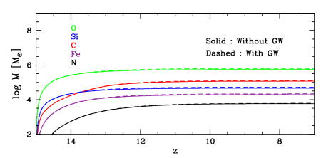
Figure 8: Mass of some elements present in the ISM versus redshift, for a $10^{9}\mbox{$M_{\odot}$}$ galaxy with a star formation efficiency $f_{*}=0.1$ and an exponential SFR. The colors corresponds to various elements, as indicated. Solid lines: simulation without galactic wind; dashed lines: simulation with galactic wind.

We performed two simulations, one with our basic model, and another one in which we turned off the galactic wind. Figure 8 shows the abundances of a few elements in the ISM. Most of the ISM enrichment occurs between redshifts $z=15$ and $z=13$, during the epoch of intense SNe activity. At lower redshifts, the enrichment by stellar winds dominates. The effect of the galactic wind is very small. Adding the wind results in a 10% increase in ISM metallicity, caused by the removal of low-metallicity ISM during the early stages of the wind. The effect the galactic wind can be much more significant but this requires a smaller galactic mass $M_{\rm gal}$ or a larger star formation efficiency $f_{*}$, or SFR much more extended in time than the ones we have considered.

In the next three subsections, we explore the parameter space by varying, respectively, the SFR, the star formation efficiency $f_{*}$, and the mass $M_{\rm gal}$ of the galaxy.

5.1 Star Formation Rate

Figure 9 shows the mass returned to the ISM by stellar winds and SNe, versus redshift, for the different SFRs. With an instantaneous SFR, there is only one stellar population and the mass loss profile is identical to the one provided by SB99. Stellar winds are absent in this case because all the stars were formed in a metal-free ISM. For the constant SFR, the increase in mass returned to the ISM is caused by the formation of more and more stars. Since SNe dominate over stellar winds, a plateau is eventually reached when the time of the simulation is equal to the lifetime of the SNe for the first generation of stars. After that moment, the contribution of a new population is compensated by the death of an old population. The processus is the same for the exponential SFR, except that the mass of the stellar populations decreases with time. Hence, the death of an old population is replaced by the birth of a less-massive population, which explains the absence of a plateau. For the constant SFR, there is a sudden drop at $z=10.7$ which corresponds to the last SNe explosions. The material ejected after that corresponds to the giant phase of low-mass stars.

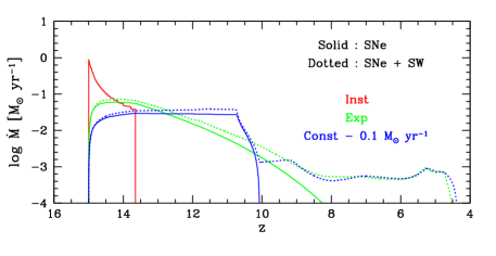
Figure 9: Mass loss rate of stars versus redshift, for a $10^{9}\mbox{$M_{\odot}$}$ galaxy with a star formation efficiency $f_{*}=0.1$. The various colors represent different SFRs, as indicated. Solid lines: simulations with SNe only; dotted lines: simulations with SNe and stellar winds.

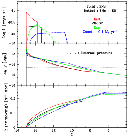
Figure 10: Luminosity (top panel), internal pressure (middle panel), and comoving radius of the galactic wind (bottom panel) versus redshift, for a $10^{9}\mbox{$M_{\odot}$}$ galaxy with a star formation efficiency $f_{*}=0.1$. Colors and linetypes have the same meaning as in Figure 9. The solid black lines show, for comparison, the model of PMG07. The dotted black line in the middle panel shows the external pressure of the IGM.

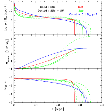
Figure 11: Density profile (top), cumulative mass profile (middle), and metallicity profile (bottom) of material ejected into the IGM by the galactic wind, at $z=0$, for a $10^{9}\mbox{$M_{\odot}$}$ galaxy with a star formation efficiency $f_{*}=0.1$. Colors and linetypes have the same meaning as in Figures 9 and 10. The dashed curves show the results for an exponential SFR with minimum SNe progenitor masses $M_{i}=6\mbox{$M_{\odot}$}$ and $M_{i}=10\mbox{$M_{\odot}$}$. In the top panel, the horizontal dashed line shows the density of the IGM inside the cavity, assuming $f_{m}=0.1$.

Figure 10 shows the luminosity, internal pressure, and comoving radius of the galactic wind, for the various SFRs. Again, stellar winds do not have much effect on the results. One interesting aspect is that an extended period of star formation tends to produce a larger final radius for the outflow, compared with an instantaneous SFR, even though the total stellar mass $M_{*}$ formed is the same. The top panel of Figure 11 shows the density profiles of the galactic wind. The density gradients are very strong, with the density dropping by $3-5$ orders of magnitude from the center to the edge. This is caused mostly by the dilution resulting from the expansion. The outer density profile is lower for the constant SFR than for the instantaneous and exponential ones. In our galactic wind model, the outer parts of the wind contain gas that was expelled by the galaxy at early time. The amount of material ejected during the early phases will depend of the mass loss rate $\dot{M}_{\rm GW}$ at that time, which is proportional to $L(t)$ [eq. (25)]. As Figure 10 shows, in the early phases, $L(t)$ is larger for the instantaneous and exponential SFR’s than for the constant SFR, which leads to a larger amount of material being ejected, material which ends up in the outer parts of the wind. The dashed line shows the density of the IGM inside the cavity, assuming $f_{m}=0.1$. Not surprisingly, the wind density exceeds the IGM density inside the galaxy, or immediately outside it. But at larger radii, the wind density drops several orders of magnitude below the IGM density. We calculated the mass of the IGM inside the cavity, assuming a shell thickness $\delta=0.05$. For the 5 cases plotted in Figure 11, the values are in the range $3.86-7.27\times 10^{8}\mbox{$M_{\odot}$}$. The mass added by the galactic wind is $2.73\times 10^{7}\mbox{$M_{\odot}$}$, or between 3.8% and 7.1% of the mass in the cavity. This justifies a posteriori the assumption made by TSE that the mass added by the wind can be neglected.

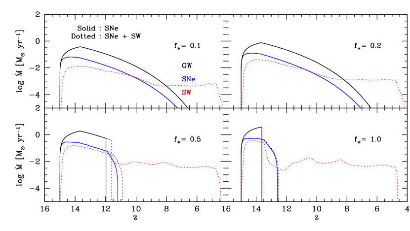
Figure 12: Rate of mass loss by SNe (blue), stellar winds (red), and galactic wind (black) versus redshift, for a $10^{9}\mbox{$M_{\odot}$}$ galaxy with an exponential SFR. Solid lines: simulations with SNe only; dotted lines: simulations with SNe and stellar winds. The various panels correspond to different star formation efficiencies $f_{*}$, as indicated. In the top panels, the solid and dotted lines are indistinct for the galactic winds and SNe.

The middle panel of Figure 11 shows the cumulative mass profile of the galactic wind, that is, the mass $M_{\rm GW}(r)$ between 0 and $r$. Even though the density is maximum in the center, the actual amount of ejecta located near the galaxy is negligible. For a galaxy of mass $10^{9}M_{\odot}$, collapsing at redshift $z=15$, the virial radius is $r_{200}=2\,{\rm kpc}$, and the radius of the stellar component is even smaller. Essentially all the gas contained in the galactic wind has been ejected from the galaxy, and most of it is located at radius $r>100\,{\rm kpc}$.

The bottom panel of Figure 11 shows the metallicity profiles. The metallicity gradients have a different origin, since the dilution caused by the expansion of the wind equally affects metals, hydrogen, and helium. Since the material located in the outer parts of the wind was ejected earlier than material located in the inner parts, the metallicity gradient simply reflects the time-evolving chemical composition of the ISM. With an instantaneous SFR, the ISM is enriched in metals very rapidly. Hence, the gas ejected into the galactic wind at early times is already metal-rich. As a result, the metallicity in the outer parts of the wind is larger for the instantaneous SFR than for the other SFRs.

The dashed curves in Figure 11 show the effect of changing the minimum SNe progenitor mass (for an exponential SFR). Lowering the minimum mass from $8\mbox{$M_{\odot}$}$ to $6\mbox{$M_{\odot}$}$ increase the final radius of the outflow by 12% and the total mass ejected by 59%. Increasing the minimum mass to $10\mbox{$M_{\odot}$}$ reduces the final radius of the outflow by 8% and the total mass ejected by 21%.

5.2 Efficiency of the Star Formation

Figure 12 shows the effect of varying the efficiency of star formation for a $10^{9}\mbox{$M_{\odot}$}$ galaxy with an exponential SFR. Apart from the fact that the mass loss rate increases with the number of stars formed, the most striking feature of this figure is that, for $f_{*}\geq 0.5$, the galactic wind can be sufficiently powerful to eject the totality of the ISM. Eventually, the ISM is replenished by SN ejecta and stellar winds produced by stars already formed. Figure 13 shows that stellar winds are more significant with $f_{*}=0.5$ than with $f_{*}=1$. Lowering $f_{*}$ spreads star formation over a longer period of time, enabling stars to form in an environment richer in metals, and resulting in stronger stellar winds.

Figure 14 shows the evolution of the ISM metallicity. The metallicity increases faster with a higher star formation efficiency, since there are more stars available to enrich the ISM. When all the gas in the galaxy is eventually ejected into the IGM, the metallicity experiences a sudden increase before reaching a maximum value. This sudden increase occurs when the mass remaining into the ISM becomes similar to the mass returned by stars. Then, the mass of the ISM keeps dropping, and the metallicity approaches the value corresponding to the last stellar ejecta. Afterward, the metallicity decreases because the last SNe ejected fewer and fewer metals. Then, when stellar winds are taken into account, the metallicity of the ISM continue to decrease with time because low-mass stars in their giant phases eject material composed mostly of hydrogen and helium.

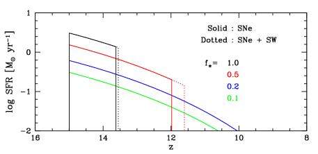
Figure 13: Rate of mass converted to stars versus redshift, for a $10^{9}\mbox{$M_{\odot}$}$ galaxy with an exponential SFR. Solid lines: simulations with SNe only; dotted lines: simulations with SNe and stellar winds. The various colors correspond to different star formation efficiencies $f_{*}$, as indicated. For $f_{*}=0.2$ and 0.1, the solid and dotted lines are indistinct.

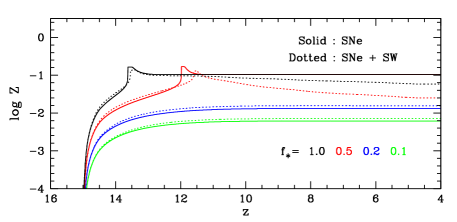
Figure 14: Metallicity of the ISM versus redshift, for a $10^{9}\mbox{$M_{\odot}$}$ galaxy with an exponential SFR. Colors and linetypes have the same meaning as in Figure 13.

Figure 15 shows the evolution of the composition of the ISM. The importance of stellar winds becomes naturally larger when the star formation efficiency increases. The stellar winds do not have much effect on the total mass of the ISM. However, there is a significant difference in the abundances of carbon and nitrogen for $f_{*}>0.1$. Figure 16 shows the density of various elements inside the galactic wind. The external part of the galactic wind has the composition of the ISM during the early phases. To have a significant effect on the composition of the external regions of the galactic wind, which are the prime contributor to the IGM enrichment, the enrichment of the ISM must happen rapidly, which is the case when $f_{*}$ is large. Figure 17 shows th metallicity profile of the galactic wind, for the various values of $f_{*}$. The amount of metal ejected into the IGM seems large enough to fit observations. Various studies indicate that the IGM metallicity at redshifts between 2.5 and 3.5 is of the order of $10^{-2.5}Z_{\odot}$ (Songaila & Cowie, 1996; Hellsten et al., 1998; Rauch et al., 1997; Davé et al., 1998).

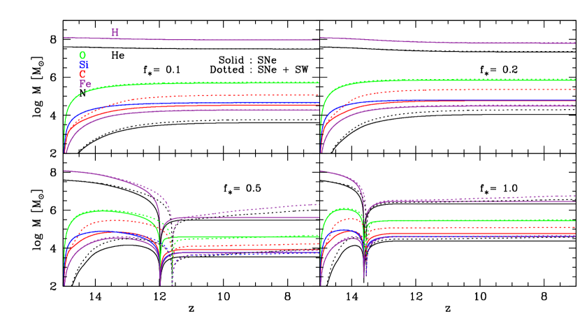
Figure 15: Mass of various elements present in the ISM versus redshift, for a $10^{9}\mbox{$M_{\odot}$}$ galaxy with an exponential SFR. The various panels correspond to different star formation efficiencies $f_{*}$, as indicated. The colors corresponds to various elements, as indicated. Solid lines: simulations with SNe only; dotted lines: simulations with SNe and stellar winds.

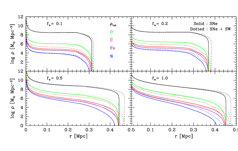
Figure 16: Density profile of material ejected in the IGM, for a $10^{9}\mbox{$M_{\odot}$}$ galaxy with an exponential SFR. Black lines: total density; colored lines: density of various elements, as indicated. Linetypes have the same meaning as in Figure 15.

5.3 The Mass of the Galaxy

Usually, the evolution of the ISM is unaffected by the mass of the host galaxy. Increasing the mass of the galaxy increases the mass of the ISM, the mass in stars, the amount of gas ejected by SNe and stellar winds, and the amount of metals ejected by exactly the same factor. The only thing that might affect this tendency is the mass loss caused by the galactic wind. If the power of the wind is moderate, the evolution of the ISM will be unaffected. This is the case for the most massive galaxies, because the energy deposited is less and less coherent, which reduces the fraction of energy $f_{w}$ used to produce the galactic wind. For less massive galaxies, the ISM is more enriched, because the galactic wind expels more gas, which increases the relative importance of metals returned by stars.

Figure 18 shows the comoving radius of the galactic wind, for galaxies of various masses, all having $f_{*}=0.1$ and an exponential SFR. The final radius increases with the mass, but this effect is weak and gets weaker at larger masses. The radius of the galactic wind $R$ increases by a factor of 1.6 from $10^{8}\mbox{$M_{\odot}$}$ to $10^{9}\mbox{$M_{\odot}$}$, and 1.13 from $10^{9}\mbox{$M_{\odot}$}$ to $10^{10}\mbox{$M_{\odot}$}$. This results from the competition between several effects. The energy deposited into the ISM by SNe and stellar winds increases linearly with $M_{\rm gal}$, but the fraction $f_{w}$ of that energy which is used to power the wind decreases with $M_{\rm gal}$. At large masses, $f_{w}\propto 1/M_{\rm gal}$ and the two effects cancel out. At smaller masses, $f_{w}$ decreases slower than $1/M_{\rm gal}$ and the energy available to power the wind increases with mass. That energy must compete with the gravitational pull of the galaxy [last term in eq. (34)], which increases with galactic mass. This effect reduces further the final radius of the wind, and at large masses $R$ actually decreases with increasing mass. We do not include masses $M_{\rm gal}=10^{11}\mbox{$M_{\odot}$}$ and $10^{12}\mbox{$M_{\odot}$}$ in Figure 18, because the galactic wind does not even start for those objects. With an instantaneous SFR, we can maximize the effect of the energy deposition and produce a wind from $M_{\rm gal}=10^{11}\mbox{$M_{\odot}$}$, but this wind remains gravitationally bound to the galaxy and eventually falls back.

6 SUMMARY AND CONCLUSION

We have combined a population synthesis code, interpolation tables for the mass and composition of SN ejecta, and an analytical model for galactic winds into a single algorithm that self-consistently describes the evolution of starburst galaxies. This model describes the evolution of the stellar populations in the galaxy, the evolution of the mass and chemical composition of the ISM, the propagation of the galactic wind, and the distribution and abundances of metals inside the galactic wind. In particular, the algorithm (1) provides a detailed calculation of the energy deposited into the ISM by SNe and stellar winds, which is responsible for driving the galactic wind, (2) takes into account the time-evolution of the chemical composition of the ISM, which directly affect the composition of the galactic wind, and (3) takes into account the removal of the ISM by galactic winds, which affects the metallicity of the ISM, and the metallicity of the stellar populations to follow.

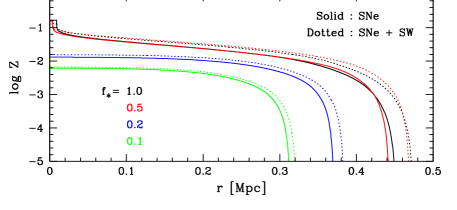
Figure 17: Metallicity profile of material ejected in the IGM at $z=0$, for a $10^{9}\mbox{$M_{\odot}$}$ galaxy with an exponential SFR. The various colors represent different star formation efficiencies $f_{*}$. Colors and linetypes have the same meaning as in Figures 13 and 14.

Figure 18: Comoving radius of galactic wind versus redshift, for galaxies with an exponential SFR and a star formation efficiency $f_{*}=0.1$, for various galaxy masses $M_{\rm gal}$ in solar masses. Solid lines: simulations with SNe only; dotted lines: simulations with SNe and stellar winds.

Our first results concern the SFR for the galaxy. For a given star formation efficiency $f_{*}$, a longer SFR tends to produce a galactic wind that reaches a larger extent, but this wind will be less dense. By increasing the star formation efficiency, we can produce a wind that reaches a larger extent and has a higher metallicity near its front. In some cases, the energy deposited by the stars is sufficient to completely expel the ISM. When it happens, star formation is shut down, and the galactic wind enters the post-SN phase prematurely. Hence, paradoxically, an increase in the star formation rate can sometimes result in a galactic wind that reaches a smaller extend. This happens with galaxies of masses $M_{\rm gal}=10^{8}\mbox{$M_{\odot}$}$ or less, because their shallow potential well enables the complete removal of the ISM by the galactic wind.

For galaxies with mass above $10^{11}\mbox{$M_{\odot}$}$, the material ejected in the IGM always falls back onto the galaxy, no matter the value of $f_{*}$. Therefore, in the case of energy-driven galactic winds, lower-mass galaxies are more likely to be the ones responsible for enriching the IGM and potentially perturbing the formation of nearby galaxies. Below $10^{11}\mbox{$M_{\odot}$}$, the extent of the galactic wind and its mass and metal content both increase with the mass of the galaxy at constant $f_{*}$. With different values of $f_{*}$, a less massive galaxy can sometimes produce a larger wind.

Our current model does not take into account the effect of Type Ia SNe. These are difficult to include, because of the uncertainties on the lifetime of the progenitors. The simulations presented in this paper start at redshift $z=15$, and end between redshifts $z=9$ and 6. The corresponding time periods are shorter than $1\,{\rm Gyr}$, which is shorter than the lifetime of several Type Ia progenitors. The energy produced by Type Ia SNe is about 20% of the energy produced by Type II SNe (see Fig. 10 of Benson 2010). Hence, including the Type Ia SNe would result in a slightly larger final radius for the outflow. A Type Ia SNe can produce up to 7 times more iron than a Type II SNe (see model W7 in Nomoto et al. 1997), and their contribution to the iron enrichment of the ISM become important after $1\,{\rm Gyr}$ (Wiersma, 2010). Hence, the abundances of iron we present in this paper are underestimated. But because of the delay, the additional iron produced would remain in the inner parts of the galactic wind.

We have assumed a minimum value of $M_{i}=8\mbox{$M_{\odot}$}$ for the minimum mass of SNe progenitors. However, the correct value is actually quite uncertain. We did a few simulations with minimum masses of $6\mbox{$M_{\odot}$}$ and $10\mbox{$M_{\odot}$}$. Our preliminary results show differences of order 10% in the final radius of the outflow, and of order 20-60% in the total mass ejected, with the largest effect occurring when $M_{i}$ is reduced. We intend to study this in more detail in the future.

To conclude, properties of galactic winds depend on the host galaxy properties, such as the mass or star formation efficiency. The history of the ISM enrichment plays a determinant role in the chemical composition and extent of the galactic wind, and therefore its ability to enrich the IGM. The next step will consist of implementing this galactic outflow model into large-scale cosmological simulations of galaxy formation and the evolution of the IGM. These will be the first simulation of this kind to include a detailed treatment of the stellar winds and their impact on the chemical enrichment of the IGM

References

- Aguirre et al. (2008) Aguirre, A., Dow-Hygelund, C., Schaye, J., & Theuns, T. 2008, ApJ, 689, 851
- Babul et al. (2002) Babul, A., Balogh, M. L., Lewis, G. F., & Poole, G. B. 2002, MNRAS, 330, 329
- Barai et al. (2011) Barai, P., Martel, H., & Germain, J. 2011, ApJ, 727, 54
- Baugh (2006) Baugh, C. M. 2006, Rep.Prog.Phys., 69, 3101
- Behroozi et al. (2010) Behroozi, P. S., Conroy, C., & Wechsler, R. H. 2010, ApJ, 717, 379
- Belczynski et al. (2010) Belczynski, K., Bulik, T., Fryer, C. L., Ruiter, A., Valsecchi, F., Vink, J. S., & Hurley, J. R. 2010, ApJ, 714, 1217
- Benson (2010) Benson, A. 2010, Phys. Rep., 495, 33
- Blumenthal et al. (1984) Blumenthal, G. R., Faber, S. M., Primack, J. R., & Rees, M. J. 1984, Nature, 311, 517
- Cavaliere et al. (1997) Cavaliere, A., Menci, N., & Tozzi, P. 1997, ApJ, 484, L21
- Cen et al. (2005) Cen, R., Nagamine, K., & Ostriker, J. P. 2005, ApJ, 635, 86
- Chieffi & Limongi (2004) Chieffi, A., & Limongi, M. 2004, ApJ, 608, 405
- Davé et al. (1998) Davé, R., Hellsten, U., Hernquist, L., Katz, N., & Weinberg, D. H. 1998, ApJ, 509, 661
- Evrard & Henry (1991) Evrard, A. E., & Henry, J. P. 1991, ApJ, 383, 95
- Furlanetto & Loeb (2001) Furlanetto, S. R., & Loeb, A. 2001, ApJ, 556, 619
- Germain et al. (2009) Germain, J., Barai, P., & Martel, H. 2009, ApJ, 704, 1002
- Hameed et al. (2001) Hameed, S., Blank, D. L., Young, L. M., & Devereux, N. 2001, ApJL, 546, 97
- Heger & Woosley (2010) Heger, A., & Woosley, S. E. 2010, ApJ, 724, 341 (HW10)
- Hellsten et al. (1998) Hellsten, U., Davé, R., Hernquist, L., Weinberg, D. H., & Katz, N., 1997, ApJ, 487, 482
- Horiuchi et al. (2011) Horiuchi, S., Beacom, J. F., Kochanek, C. S., Prieto, J. L., Stanek, K. Z., & Thompson, T. A. 2011, preprint (arXiv:1102.1977v1)
- Isobe et al. (1990) Isobe, T., Feigelson, E. D., Akritas, M., & Babu, G. J. 1990, ApJ, 364, 104
- Jamet et al. (2010) Jamet, L., Cerviño, M., Luridiana, V., Pérez, E., & Yakobchuk, T. 2010, A&A, 509, 10
- Kaiser (1991) Kaiser, N. 1991, ApJ, 383, 104
- Kollmeier et al. (2006) Kollmeier, J. A., Miralda-Escudé, J., Cen, R., & Ostriker, J. P. 2006, ApJ, 638, 52
- Kroupa (2001) Kroupa, P. 2001, MNRAS, 322, 231
- Krticka (2006) Krticka, J. 2006, MNRAS, 367, 1282
- Leitherer & Heckman (1995) Leitherer, C., & Heckman, T. M. 1995, ApJS, 96, 9
- Leitherer et al. (1992) Leitherer, C., Robert, C., & Drissen, L. 1992, ApJ, 401, 596
- Leitherer et al. (1999) Leitherer, C., Schaerer, D., Goldader, J. F., González Delgado, R. M., Robert, C., Kune, D. F., de Mello, D. F., & Heckman, T. M. 1999, ApJS, 123, 3
- Levine & Gnedin (2005) Levine, R., & Gnedin, R. Y. 2005, ApJ, 632, 727
- Limongi & Chieffi (2007) Limongi, M., & Chieffi, A. 2007, in The Multicolored Landscape of Compact Objects and Their Explosive Origins. AIP Conference Proceedings, Volume 924, p. 226
- Limongi & Chieffi (2008) Limongi, M., & Chieffi, A. 2008, EAS Publication Series, Volume 32, p. 233
- Madau et al. (2001) Madau, P., Ferrara, A., & Rees, M. J. 2001, ApJ, 555, 92
- Martin (1999) Martin, C. L. 1999, ApJ, 513, 156
- Martinez-Serrano et al. (2008) Martinez-Serrano, F. J., Serna, A., Dominguez-Tenreiro, R., & Molla, M. 2008, MNRAS, 388, 39
- McKee (1990) McKee, C. F. 1990, The Evolution of the ISM, ed. L. Blitz (Provo: Brigham Young University), p. 3
- Meyer & York (1987) Meyer, D. M., & York, D. G. 1987, ApJ, 315, L5
- Mokiem et al. (2007) Mokiem, M. R., et al. 2007, A&A, 473, 603
- Murray et al. (2005) Murray, N., Quataert, E., & Thompson, T. A. 2005, ApJ, 618, 569
- Nomoto et al. (1997) Nomoto, K., et al. 1997, Nucl.Phys.A, 621, 467
- Nomoto et al. (2006) Nomoto, K., Tominaga, N., Umeda, H., Kobayashi, C., & Maeda, K. 2006, Nucl.Phys.A, 777, 424 (N06)
- Oppenheimer & Davé (2006) Oppenheimer, B. D., & Davé. R. 2006, MNRAS, 373, 1265
- Oppenheimer & Davé (2008) Oppenheimer, B. D., & Davé. R. 2008, MNRAS, 387, 577
- Péquignot (2008) Péquignot, D. 2008, A&A, 478, 371
- Pieri et al. (2010a) Pieri, M. M., Frank, S., Mathur, S., Weinberg, D. H., York, D. G., & Oppenheimer, B. D. 2010a, ApJ, 716, 1084
- Pieri et al. (2010b) Pieri, M. M., Frank, S., Mathur, S., Weinberg, D. H., & York, D. G. 2010b, 724, 69L
- Pieri & Haehnelt (2004) Pieri, M. M., & Haehnelt, M. G. 2004, MNRAS, 347, 985
- Pieri et al. (2007) Pieri, M. M., Martel, H., & Grenon, C. 2007, ApJ, 658, 36 (PMG07)
- Pinsonneault et al. (2010) Pinsonneault, S., Martel, H. & Pieri, M. M. 2010, ApJ, 725, 208
- Rauch et al. (1997) Rauch, M., Haehnelt, M. G., & Steinmetz, M. 1997, ApJ, 481, 601
- Samui et al. (2008) Samui, S., Subramanian, K., & Srianand, R. 2008, MNRAS, 385, 783
- Scannapieco & Broadhurst (2001) Scannapieco, E., & Broadhurst, T. 2001, ApJ, 549, 28
- Scannapieco et al. (2002) Scannapieco, E., Ferrara, A., & Madau, P. 2002, ApJ, 574, 590
- Scannapieco & Oh (2004) Scannapieco, E., & Oh, S. P. 2004, ApJ, 608, 62
- Scannapieco et al. (2001) Scannapieco, E., Thacker, R. J., & Davis, M. 2001, ApJ, 557, 605
- Scannapieco et al. (2005) Scannapieco, E., Tissera, P. B., White, S. D. M., & Springel, V. 2005, MNRAS, 364, 552
- Schaye et al. (2003) Schaye, J., Aguirre, A., Kim, T., Theuns, T., Rauch, M., & Sargent, W. L. W. 2003, ApJ, 596, 768
- Sharp & Bland-Hawthorn (2010) Sharp, R. G., & Bland-Hawthorn, J. 2010, ApJ, 711, 818
- Songaila & Cowie (1996) Songaila, A., & Cowie, L. L. 1996, ApJ, 112, 335
- Springel & Hernquist (2003) Springel, V., & Hernquist, L. 2003, MNRAS, 312, 334
- Tegmark et al. (1993) Tegmark, M., Silk, J., & Evrard, A. 1993, ApJ, 417, 54
- Theuns et al. (2002) Theuns, T., Viel, M., Kay, S., Schaye, J., Carswell, R. F., & Tzanavaris, P. 2002, ApJ, 578, L5
- Tornatore et al. (2007) Tornatore, L., Borgani, S., Dolag, K., & Matteucci, F. 2007, MNRAS, 381, 1050
- Tozzi & Norman (2001) Tozzi, P., & Norman, C. 2001, ApJ, 546, 63
- Vázquez & Leitherer (2005) Vázquez, G. A., & Leitherer, C. 2005, ApJ, 621, 695
- Veilleux et al. (2005) Veilleux, S., Cecil, G., & Bland-Hawthorn, J. 2005, ARA&A, 43, 769
- Vink & de Koter (2005) Vink, J, S., & de Koter, A. 2005, A&A, 442, 587
- Vink et al. (2001) Vink, J, S., de Koter, A., & Lamers, H. J. G. L. M. 2001, A&A, 369, 574
- Voit et al. (2002) Voit, M. G., Bryan, G. L., Balogh, M. L., & Bower, R. G. 2002, ApJ, 576, 601
- Westmoquette et al. (2009) Westmoquette, M. S., Smith, L. J., Gallagher, J. S., & Exter, K. M. 2009, Ap&SS, 324, 187
- Wiersma (2010) Wiersma, R. 2010, PhD Thesis, University of Leiden
- Woosley & Heger (2007) Woosley, S. E., & Heger, A., 2007, Phys.Rep., 442, 269 (WH07)
- Woosley et al. (2002) Woosley, S. E., Heger, A., & Weaver, T. A. 2002, Rev.Mod.Phys., 74, 1015
- Woosley & Weaver (1995) Woosley, S. E., & Weaver, T. A. 1995, ApJS, 101, 181
- Zhan et al. (2008) Zhan, W., Woosley, S. E., & Heger, A. 2008, ApJ, 679, 639