Time-dependent density functional theory for strong electromagnetic fields in crystalline solids

Abstract

We apply the coupled dynamics of time-dependent density functional theory and Maxwell equations to the interaction of intense laser pulses with crystalline silicon. As a function of electromagnetic field intensity, we see several regions in the response. At the lowest intensities, the pulse is reflected and transmitted in accord with the dielectric response, and the characteristics of the energy deposition is consistent with two-photon absorption. The absorption process begins to deviate from that at laser intensities $\sim 10^{13}$ W/cm², where the energy deposited is of the order of 1 eV per atom. Changes in the reflectivity are seen as a function of intensity. When it passes a threshold of about $3\times 10^{12}$ W/cm², there is a small decrease. At higher intensities, above $2\times 10^{13}$ W/cm², the reflectivity increases strongly. This behavior can be understood qualitatively in a model treating the excited electron-hole pairs as a plasma.

I Introduction

The Maxwell equations describe propagation of electromagnetic fields in bulk matter taking into account the material properties by the constitutive relations. For ordinary light pulses, the response of the medium is linear in the electromagnetic field and is characterized by the linear susceptibilities. In recent experiments with intense and ultrashort laser pulses, however, one often encounter conditions which require theoretical treatments beyond the linear response. If the perturbative expansion is no longer useful, one need to go back to the time-dependent Schrödinger equation for electrons and to solve it in time domain.

In the last two decades, computational approaches to solve the time-dependent Schrödinger equation under intense electric fields have been developed for atoms and small molecules kr92 ; ch92 ; ka99 . For electron dynamics in bulk matter as well as in molecules, one often needs to go to the less demanding approach based on time-dependent density-functional theory (TDDFT) pe99 ; ca00 ; to01 ; no04 ; ca04 ; ot08 ; sh10 ; mi10 . We consider the TDDFT is the only ab-initio quantum method applicable to high fields in condensed media.

In this paper, we develop a formalism and computational method to describe propagation of intense electromagnetic field in the condensed medium incorporating feedback of electron dynamics to the electromagnetic field. This requires a consistent treatment of electrons and the electromagnetic field in coupled equations of motion. Such attempts have been undertaken by several groups, for isolated molecules fr11 , nano-particles iw09 ; iw10 ; ch10 , and gases lo07 .

Experimentally, electron-hole plasmas are generated by irradiating solids with strong laser pulses, and the threshold for dielectric breakdown has been measured re92 ; vo96 ; le98 ; so00 ; hu01 ; na02 ; ma04 ; ra05 ; da06 ; wi06 . To describe the phenomena, model approaches such as a rate equation for electronic excitations have been developed re04 ; pe05 ; re06 ; ha07 ; pe08 ; me10 . For this problem, we have developed a first-principles approach ot08 ; ot09 . We calculated dielectric breakdown in crystalline diamond ot08 and quartz ot09 , using TDDFT and treating the electric field as a longitudinal field. The calculated dielectric breakdown threshold was much higher than observed. In the present work, we improve the theory by incorporating both magnetic and electric fields in the equations, permitting a proper description of transverse electromagnetic wave propagation.

Our formal development gives a way to separate out the two spatial scales that must be treated simultaneously. The electron dynamics is calculated on the atomic scale, resolving position dependences of some tenths of an atomic unit. The electronic field is decomposed into two parts, one on the atomic scale and the other on the scale of the electromagnetic wave length. The atomic scale field is very similar from one unit cell to neighboring cells of the crystal. The other part of the field gives the large scale variation needed to describing the electromagnetic self-coupling and wave propagation. We introduce two grid systems with different resolution for this problem.

The construction of the paper is as follows. In Sec. 2, we present our formalism of multi-scale description for coupled dynamics of electrons and electromagnetic fields. In Sec. 3, numerical methods are explained. In Sec. 4, calculated results are presented. We provide an interpretation for the electron dynamics at the surface in terms of the electron-hole plasma. We also compare dynamics of the present multi-scale calculation with the microscopic dynamics in longitudinal and transverse geometries. Finally, a summary is presented in Sec. 5.

II Formalism

II.1 Macroscopic equations for electromagnetic fields

We will consider a coupled dynamics of electrons and electromagnetic field in bulk crystalline solid allowing for strong electromagnetic fields. We immediately recognize there are two different spatial scales in the problem. The spatial scale of electromagnetic field is set by laser wavelength, of the order 1 $\mu$m. The spatial scale of electron dynamics is much smaller, of the order of $10^{-1}$ nm. We are thus led to a multi-scale description for the problem, employing two spatial grids of different grid sizes. We will use the notation $\mathbf{R}$ and $\vec{r}$ for the macroscopic and microscopic coordinates, respectively.

The essence of our method is to use the freedom to choose the electromagnetic gauge to separate the two scales. In the expression for the electric field,

$$\vec{E}=-\vec{\nabla}\phi-{1\over c}{\partial\vec{A}\over\partial t}$$ (1)

the gauge field $\vec{A}$ contains all the macroscopic electromagnetic physics. The microscopic physics, to be calculated on a unit cell of the lattice, uses both $\vec{A}$ and the scalar potential $\phi$.

To derive the theory formally, we start by taking a specific gauge condition, the scalar potential $\phi$ is set equal to zero. In this gauge, we have the following equations for the vector potential $\vec{A}(\vec{r},t)$,

$$-\frac{1}{c}\frac{\partial}{\partial t}\vec{\nabla}\vec{A}=4\pi e\left(n_{ion}-n\right),$$ (2)

$$\frac{1}{c^{2}}\frac{\partial^{2}\vec{A}}{\partial t^{2}}-\nabla^{2}\vec{A}+\vec{\nabla}\left(\vec{\nabla}\cdot\vec{A}\right)=-\frac{4\pi e}{c}\vec{j}.$$ (3)

Here we introduced the ionic density given by

$$n_{ion}(\vec{r})=\sum_{\alpha}Z_{\alpha}\delta(\vec{r}-\vec{R}_{\alpha}),$$ (4)

where $\vec{R}_{\alpha}$ and $Z_{\alpha}$ are the coordinate and charge number of $\alpha$-th ion, respectively. We ignore the motion of ions throughout this paper. $n$ and $\vec{j}$ are the number density and current of electrons, respectively, and satisfy the equation of continuity,

$$\frac{\partial}{\partial t}n+\vec{\nabla}\vec{j}=0.$$ (5)

We note that longitudinal part of the vector potential is described redundantly by two equations (2) and (3).

We then proceed to define macroscopic quantities from the microscopic ones. As will be discussed later, the microscopic density and current are obtained from the time-dependent Kohn-Sham orbitals. The macroscopic version of these quantities, $N_{\mathbf{R}}(t)$ and $\vec{J}_{\mathbf{R}}(t)$, may be defined in principle by applying some smoothing function to the microscopic quantities. In practice, we define this by averaging over the unit cell of the lattice. The macroscopic density and current also satisfies the equation of continuity. We will not need it for the geometry considered below, but it would be needed for other geometries.

We obtain macroscopic vector potential from $\vec{A}(\vec{r},t)$ by a smoothing procedure which we denote as $\vec{A}_{\mathbf{R}}(t)$. It satisfies the equations

$$-\frac{1}{c}\frac{\partial}{\partial t}\vec{\nabla}_{\mathbf{R}}\vec{A}_{\mathbf{R}}(t)=-4\pi eN_{\mathbf{R}}(t),$$ (6)

$$\frac{1}{c^{2}}\frac{\partial^{2}}{\partial t^{2}}\vec{A}_{\mathbf{R}}(t)-\vec{\nabla}^{2}_{\mathbf{R}}\vec{A}_{\mathbf{R}}(t)+\vec{\nabla}_{\mathbf{R}}\left(\vec{\nabla}_{\mathbf{R}}\cdot\vec{A}_{\mathbf{R}}(t)\right)=-\frac{4\pi e}{c}\vec{J}_{\mathbf{R}}(t),$$ (7)

This is our basic equation to describe a propagation of macroscopic electromagnetic field.

For a microscopic physics, we treat the macroscopic field as uniform and otherwise we retain only a longitudinal part of the vector potential. Physically, the approximation is to neglect the transverse current and variation of the magnetic field within the unit cells. The neglect of transverse current amounts to ignore the orbital magnetization. The neglect of magnetic field effects on electrons may be justified when the velocity of electrons accelerated by the laser pulse is much smaller than the velocity of light. As will be explained later, we will employ a periodic scalar potential instead of the longitudinal vector potential for the microscopic description in the unit cells.

In general, the presence of boundaries requires special attention. If we may assume that a surface charge is localized in a sufficiently thin layer at a surface, we may treat it as a discontinuity of the macroscopic vector potential at the surface. Let us consider a small volume around a point ${\mathbf{R}}$ at a surface and apply the Gauss theorem to Eq. (6). We obtain

$$\vec{n}\cdot\left(\vec{A}_{out,\mathbf{R}}-\vec{A}_{in,\mathbf{R}}\right)=4\pi ce\int^{t}dt^{\prime}\Sigma_{\mathbf{R}}(t^{\prime}),$$ (8)

where $\vec{n}$ is a unit vector normal to the surface at ${\mathbf{R}}$ and $\Sigma_{\mathbf{R}}(t)$ is the surface charge at ${\mathbf{R}}$. This equation describes the boundary condition for the macroscopic vector potential across the surface. In the geometry we consider here, however, the fields are all parallel to the surface so that the macroscopic vector potential is continuous at the surface.

II.2 Microscopic equations for electrons

For the microscopic electron dynamics, we assume a periodic band structure and apply the equations of motion of the time-dependent density functional theory. We will make several assumptions here.

First we assume that electron dynamics at different macroscopic positions may be described independently. Namely, we define Kohn-Sham orbitals at every macroscopic grid point and ignore any direct interactions between electrons belonging to different macroscopic grid points. We only take into account the interaction between electrons of different macroscopic grid points through the macroscopic vector potential $\vec{A}_{\mathbf{R}}(t)$.

Second, we assume that $N_{\mathbf{R}}(t)$ is independent of time. This condition is satisfied in the one-dimensional propagation of linearly polarized light at normal incidence on an interface, since the macroscopic current does not include any longitudinal component as discussed below. The orbitals evolve under the time-dependent Kohn-Sham equations, but the number of electrons in each cell remains the same, and in fact the orbital occupation numbers remain zero or one in the time-evolved basis.

Third, within each cell of the microscopic scale, we ignore any effects of magnetic fields on the electrons. The macroscopic vector potential $\vec{A}_{\mathbf{R}}(t)$ will be treated as a uniform field in the microscopic scale. This permits us to treat electron dynamics induced by a uniform electric field. We also ignore the transverse component of the microscopic vector potential, retaining only the longitudinal part as mentioned before.

Since all that matters are the physical fields, we are permitted to make a different choice of gauge for the microscopic fields. In Eqs. (2) and (3), we had chosen the gauge condition that removes the scalar potential. However, to take advantage of the periodicity of the lattice, we make a gauge transformation at each macroscopic grid point, expressing periodic electromagnetic field with a scalar potential $\phi$ instead of the longitudinal part of the microscopic vector potential. We denote the scalar potential at macroscopic grid point ${\mathbf{R}}$ as $\phi_{\mathbf{R}}(\vec{r},t)$, to indicate that $\mathbf{R}$ will just be a parameter in the equation of motion for $\phi$.

We denote the Kohn-Sham orbitals at a macroscopic coordinate $\mathbf{R}$ as $\psi_{i,\mathbf{R}}(\vec{r},t)$. Under above conditions and assumptions, the time-dependent Kohn-Sham (TDKS) equation may be written as

$$i\hbar\frac{\partial}{\partial t}\psi_{i,\mathbf{R}}(\vec{r},t)=\left\{\frac{1}{2m}\left(-i\hbar\nabla_{\vec{r}}+\frac{e}{c}\vec{A}_{\mathbf{R}}(t)\right)^{2}-e\phi_{\mathbf{R}}(\vec{r},t)+\frac{\delta E_{xc}}{\delta n}\right\}\psi_{i,\mathbf{R}}(\vec{r},t).$$ (9)

In solving Eq. (9), the macroscopic coordinate $\mathbf{R}$ is treated as a parameter. The Kohn-Sham Hamiltonian thus defined is periodic in space and one may introduce Bloch functions at each time step, applying periodic boundary conditions on the electron orbitals within each microscopic cellbe00 ; ot08 ; sh10 .

The electron density and current are both periodic in space and are given by

$$n_{\mathbf{R}}(\vec{r},t)=\sum_{i}|\psi_{i,\mathbf{R}}(\vec{r},t)|^{2},$$ (10)

$$\vec{j}_{\mathbf{R}}(\vec{r},t)=\frac{1}{2m}\sum_{i} \left\{\psi^{*}_{i,\mathbf{R}}(\vec{r},t)\left(-i\hbar\vec{\nabla}_{\vec{r}}+\frac{e}{c}\vec{A}_{\mathbf{R}}(t)\right)\psi_{i,\mathbf{R}}(\vec{r},t)\right.$$ (11)

$$\left.-\psi_{i,\mathbf{R}}(\vec{r},t)\left(i\hbar\vec{\nabla}_{\vec{r}}+\frac{e}{c}\vec{A}_{\mathbf{R}}(t)\right)\psi^{*}_{i,\mathbf{R}}(\vec{r},t)\right\},$$

where the sum $i$ is over occupied orbitals. The scalar potential $\phi_{\mathbf{R}}(\vec{r},t)$ satisfies the Poisson equation,

$$\nabla^{2}_{\vec{r}}\phi_{\mathbf{R}}(\vec{r},t)=-4\pi\left(en_{ion,\mathbf{R}}(\vec{r})-en_{\mathbf{R}}(\vec{r},t)\right),$$ (12)

where $n_{ion,\mathbf{R}}$ is the ionic density at macroscopic grid point ${\mathbf{R}}$.

Since the density and the current are periodic in space, the average over the unit cell is meaningful also on the macroscopic scale. The main macroscopic quantity we need from the electronic dynamics is the current, defined as

$$\vec{J}_{\mathbf{R}}(t)=\frac{1}{\Omega}\int_{\Omega}d\vec{r}\vec{j}_{\mathbf{R}}(\vec{r},t),$$ (13)

where $\Omega$ is the volume of the unit cell.

II.3 Conserved energy

To obtain an expression for the conserved energy in the present multi-scale description, we first note the above equations of motion may be derived from the following Lagrangian.

$$L=\int d{\mathbf{R}} \left[\sum_{i}\int_{\Omega}d\vec{r}\left\{\psi^{*}_{i,\mathbf{R}}i\hbar\frac{\partial}{\partial t}\psi_{i,\mathbf{R}}-\frac{1}{2m}\left|\left(-i\hbar\vec{\nabla}_{\vec{r}}+\frac{e}{c}\vec{A}_{\mathbf{R}}\right)\psi_{i,\mathbf{R}}\right|^{2}\right\}\right.$$ (14)

$$-\int_{\Omega}d\vec{r}\left\{\left(en_{ion}-en_{\mathbf{R}}\right)\phi_{\mathbf{R}}-E_{xc}[n_{\mathbf{R}}]\right\}$$

$$\left.+\int_{\Omega}d\vec{r}\frac{1}{8\pi}\left(\vec{\nabla}_{\vec{r}}\phi_{\mathbf{R}}\right)^{2}+\frac{\Omega}{8\pi c^{2}}\left(\frac{\partial\vec{A}_{\mathbf{R}}}{\partial t}\right)^{2}-\frac{\Omega}{8\pi}\left(\vec{\nabla}_{\mathbf{R}}\times\vec{A}_{\mathbf{R}}\right)^{2}\right].$$

From this Lagrangian, one may derive the following Hamiltonian,

$$H=\int d\vec{R} \left[\sum_{i}\int_{\Omega}d\vec{r}\frac{1}{2m}\left|\left(-i\hbar\vec{\nabla}_{\vec{r}}+\frac{e}{c}\vec{A}_{\mathbf{R}}\right)\psi_{i,\mathbf{R}}\right|^{2}\right.$$ (15)

$$\left.+\int_{\Omega}d\vec{r}\left\{\frac{1}{2}\left(en_{ion}-en_{\mathbf{R}}\right)\phi_{\mathbf{R}}+E_{xc}[n_{\mathbf{R}}]\right\}\right.$$

$$\left.+\frac{\Omega}{8\pi c^{2}}\left(\frac{\partial\vec{A}_{\mathbf{R}}}{\partial t}\right)^{2}+\frac{\Omega}{8\pi}\left(\vec{\nabla}_{\mathbf{R}}\times\vec{A}_{\mathbf{R}}\right)^{2}\right].$$

The energy calculated from this Hamiltonian is conserved by the equations of motion.

II.4 One-dimensional propagation

In this paper, we will consider a propagation of linearly polarized laser pulse incident normally on a bulk crystalline Si on the [110] surface with the laser electric field in [100] direction. There are two spatial regions on the macroscopic scale, vacuum and crystalline solid. We take a macroscopic coordinate system such that the surface of the crystalline solid is $xy$-plane with $z=0$. In this geometry, macroscopic quantities are uniform in both $x$- and $y$-directions. Therefore, macroscopic quantities are specified by the $z$-component of $\mathbf{R}$ which we denote ${\mathrm{Z}}$.

The macroscopic vector potential has the following form,

$$\vec{A}_{\mathbf{R}}(t)=\hat{x}A_{\mathrm{Z}}(t),$$ (16)

In the vacuum region $({\mathrm{Z}}<0)$, $A_{\mathrm{Z}}(t)$ is composed of incident and reflected waves. Inside the solid, we assume a locally dipole approximation at each macroscopic coordinate, as mentioned before. Then the macroscopic electron current is parallel to the vector potential.

$$\vec{J}_{\mathbf{R}}(t)=\hat{x}J_{\mathrm{Z}}(t).$$ (17)

We note that this form of electric current is transverse. This justifies our assumption that the macroscopic electron density $N_{\mathbf{R}}(t)$ is independent of time.

For later convenience, we summarize equations of motion in the one-dimensional geometry. The vector potential $A_{\mathrm{Z}}(t)$ satisfies the following equation,

$$\frac{1}{c^{2}}\frac{\partial^{2}}{\partial t^{2}}A_{\mathrm{Z}}(t)-\frac{\partial^{2}}{\partial Z^{2}}A_{\mathrm{Z}}(t)=-\frac{4\pi e}{c}J_{\mathrm{Z}}(t).$$ (18)

The TDKS equation is given by

$$i\hbar\frac{\partial}{\partial t}\psi_{i,\mathrm{Z}}(\vec{r},t)=\left\{\frac{1}{2m}\left(-i\hbar\vec{\nabla}_{\vec{r}}+\frac{e}{c}\hat{x}A_{\mathrm{Z}}(t)\right)^{2}-e\phi_{\mathrm{Z}}(\vec{r},t)+\frac{\delta E_{xc}}{\delta n}\right\}\psi_{i,\mathrm{Z}}(\vec{r},t),$$ (19)

with the density and current,

$$n_{\mathrm{Z}}(\vec{r},t)=\sum_{i}|\psi_{i,\mathrm{Z}}(\vec{r},t)|^{2},$$ (20)

$$\vec{j}_{\mathrm{Z}}(\vec{r},t)=\frac{1}{2m}\sum_{i}\left\{\psi^{*}_{i,\mathrm{Z}}\left(-i\hbar\vec{\nabla}_{\vec{r}}+\frac{e}{c}\hat{x}A_{\mathrm{Z}}\right)\psi_{i,\mathrm{Z}}-\psi_{i,\mathrm{Z}}\left(i\hbar\vec{\nabla}_{\vec{r}}+\frac{e}{c}\hat{x}A_{\mathrm{Z}}\right)\psi^{*}_{i,\mathrm{Z}}\right\},$$ (21)

$$J_{\mathrm{Z}}(t)=\frac{1}{\Omega}\int_{\Omega}d\vec{r}\hat{x}\vec{j}_{\mathrm{Z}}(\vec{r},t).$$ (22)

The energy per unit area $E_{\cal A}$ is a conserved quantity and is given by

$$E_{\cal A}={1\over\Omega}\int d{\mathrm{Z}} \left[\sum_{i}\int_{\Omega}d\vec{r}\frac{1}{2m}\left|\left(-i\hbar\vec{\nabla}_{\vec{r}}+\frac{e}{c}\hat{x}A_{\mathrm{Z}}\right)\psi_{i,\mathrm{Z}}\right|^{2}\right.$$ (23)

$$+\int_{\Omega}d\vec{r}\left\{\frac{1}{2}(en_{ion,\mathrm{Z}}-en_{\mathrm{Z}})\phi_{\mathrm{Z}}+E_{xc}[n_{\mathrm{Z}}]\right\}$$

$$\left.+\frac{\Omega}{8\pi}\left\{\frac{1}{c}\left(\frac{\partial A_{\mathrm{Z}}}{\partial t}\right)^{2}+\left(\frac{\partial A_{\mathrm{Z}}}{\partial\mathrm{Z}}\right)^{2}\right\}\right]\,.$$

II.5 Linear response

It is essential that the theory properly describes the propagation of electromagnetic waves in the weak field limit, if it is to be useful more generally. In weak fields the electron dynamics can be calculated perturbatively to arrive at the usual linear response. The present formalism gives the same linear response as other approaches, so the weak field limit will be correct if the dielectric function is given correctly. In our previous work, we calculated the linear response by separating $A$ into a part that arose from external sources and a part arises from the medium be00 . It is not necessary to make this separation in the present formalism. To derive the dielectric function, we note Eqs. (19), (21), and (22) describe relation between the macroscopic vector potential $A_{\mathrm{Z}}(t)$ and the macroscopic current $J_{\mathrm{Z}}(t)$. We may summarize the relation as,

$$J_{\mathrm{Z}}(t)=\int^{t}dt^{\prime}\sigma(t-t^{\prime})E_{\mathrm{Z}}(t^{\prime})=-\frac{1}{c}\int^{t}dt^{\prime}\sigma(t-t^{\prime})\frac{\partial A_{\mathrm{Z}}(t^{\prime})}{\partial t},$$ (24)

where we have introduced the electric conductivity function $\sigma(t)$. In the microscopic TDDFT calculation, the vector potential is an external variable. We may compute $J_{\mathrm{Z}}(t)$ for an arbitrary $A_{\mathrm{Z}}(t)$ and thus determine the conductivity function. Since the equation is linear, it is easy to extract the frequency-dependent conductivity $\sigma(\omega)$. The dielectric function $\epsilon(\omega)$ is then given by the usual formula

$$\epsilon(\omega)=1+\frac{4\pi i\sigma(\omega)}{\omega}.$$ (25)

Further details of calculating the dielectric function in this formalism are given in the Appendix.

Since our theory gives the same macroscopic current as in the linear response, the macroscopic equations only require the dielectric function from the microscopic dynamics. Thus, the propagation of electromagnetic waves will be given by the usual relation between wave vector $k$ and frequency $\omega$,

$$\omega=\frac{ck}{\sqrt{\epsilon(\omega)}}.$$ (26)

III Numerical

III.1 Units

For numerical quantities on the microscopic scale, we will use atomic units for length and field strengths. However, we will use micrometers for lengths on the macroscopic scale. On both scales, energies will be in eV units and time in femtosecond units. We continue to include the dimensionful quantities $m$ and $e$ in formulas even though their values are equal to one. For the laser intensity, we will use the conventional units of W/cm². The conversion factor to atomic units is 1 a.u. = $3.509\times 10^{16}$ W/cm².

III.2 Electronic scale

As in our previous applications to crystalline materialsbe00 ; ot08 , we calculate the evolution of the electron wave function in a unit cell of the crystal. The orbital wave functions are represented on a 3D spatial grid which typically has a dimension of $16^{3}$. The Si lattice constant is 10.26 a.u. giving a mesh space of $\Delta x=0.64$ a.u. A high order finite difference formula is used for the derivative calculations ch94 . The number of $k$-points in the reciprocal space cell is taken as $8^{3}$; however due to symmetry there are only 80 distinct orbitals to be calculated.

The number of $k$-points adopted here are smaller than those employed in our previous work ot08 ; sh10 . The present choice is decided from a computational feasibility. Our present scheme requires microscopic electron dynamics calculations in a number of macroscopic grid points simultaneously. Thus the present calculation consumes much more computational resources than our previous calculations of a single microscopic electron dynamics. The computational wall time with the above setting is approximately 15 hours employing 1,024 processor cores in parallel with Intel Xeon X5570 (2.93GHz). This is close to the limit of our computational capability at present. The present calculation with $8^{3}$ $k$-points may not provide fully convergent results but we do not expect this truncation to affect the physical results by more than 10 percent.

The electronic structure of each macroscopic position is initialized by the ground state Kohn-Sham orbitals. The wave functions are evolved by using the 4-th order expansion of the TDDFT evolution operator ya96 ; ya06

$$e^{-iH\Delta t}\approx\sum_{n=0}^{4}{(i\Delta t)^{n}\over n!}H^{n},$$ (27)

where $H$ is the Kohn-Sham single-particle Hamiltonian appearing in Eq. (19). The orbitals at time $t+\Delta t$ are computed by applying Eq. (27) to the orbitals at time $t$. The Kohn-Sham operator $H$ is a function of the fields $\phi$, $A$, and the density. We use a fixed-time Hamiltonian $H$ in which the scalar potential and the density are taken at time $t$ and the field $A$ is taken to be $(A(t)+A(t+\Delta t))/2$. This prescription does not require any predictor step (see below) and it gives good energy conservation over the course of the integration time.

The algorithm (27) is stable provided $\Delta t$ satisfies the conditionbe06

$$\Delta t<\sqrt{\frac{2}{9}}m(\Delta x)^{2}\approx 0.2\,\,\,{\rm a.u.}$$ (28)

We use a somewhat smaller value in the calculations below, $\Delta t=0.08$ au. In a typical run, the equations of motion are integrated for 16,000 time steps, amount to a total time $1280$ au $=31$ fs. This is sufficient to see the passage of a femtosecond laser pulse through a section of the solid. At longer times, other processes such as thermalizing collisions and ionic motion become important, and the TDDFT dynamics is no longer valid.

As in previous work, we use the adiabatic approximation, taking the time-dependent functional in TDDFT the same as the ground state functional. We use the functional of Ref. lda in the local density approximation. The electron-ion interaction is treated with a norm-conserving pseudopotential tm with a gauge correction for the nonlocal part be00 .

III.3 Macroscopic Scale

On the macroscopic scale, $A_{\mathrm{Z}}(t)$ and $J_{\mathrm{Z}}(t)$ are considered as continuous functions, but they are discretized for the numerical calculation. In the results presented in the next section, we use a mesh size of 250 au $\simeq$ 13 nm. This permits us to propagate the pulse over a distance of several $\mu$m in the medium sampling the microscopic dynamics at several hundred points. We employ 256 grid points. The integrator for Eq. (18) is straightforward, but the coupling between scales requires some care. The following update procedure is simple and conserves energy to adequate precision:

$$A_{\mathrm{Z}}(t+\Delta t):=2A_{\mathrm{Z}}(t)-A_{\mathrm{Z}}(t-\Delta t)+c^{2}\Delta t^{2}\left\{{d^{2}\over d{\mathrm{Z}}^{2}}A_{\mathrm{Z}}(t)+{4\pi e^{2}\over c}J_{\mathrm{Z}}(t)\right\},$$ (29)

where the space derivative is treated with a simple three-point formula. It also permits us to use $A_{\mathrm{Z}}(t+\Delta t)$ when updating the variables for the microscopic scale.

III.4 Laser field

We use the following functional form for the shape of the incident laser pulse,

$$E_{\mathrm{Z}}(t)=E_{0}\sin^{2}({\pi({\mathrm{Z}}-ct-{\mathrm{Z}}_{0})\over cT})\sin({\omega_{\ell}({\mathrm{Z}}-ct-{\mathrm{Z}}_{0})\over c}),\hskip 28.45274pt({\mathrm{Z}}_{0}<{\mathrm{Z}}-ct<{\mathrm{Z}}_{0}+cT).$$ (30)

Here $T=18$ fs controls the pulse width, $\omega_{\ell}=1.55$ eV/$\hbar$ is the laser frequency, and $E_{0}$ is the maximum electric field strength which is related to the laser intensity $I_{0}$ by $I_{0}=cE_{0}^{2}/8\pi$.

The corresponding gauge field is obtained by an analytic calculation of the following integral,

$$A_{\mathrm{Z}}(t)=-c\int^{t}_{-\infty}dt^{\prime}E_{\mathrm{Z}}(t^{\prime}).$$ (31)

To start calculation, we need the initial vector potential at two times. One is given by $A_{\mathrm{Z}}(t=0)$. Instead of using analytic form, we employ the following for the other,

$$A_{\mathrm{Z}}(\Delta t)=A_{\mathrm{Z}}(0)+\Delta t\frac{\partial A_{\mathrm{Z}}}{\partial t}(0)+\frac{1}{2}c^{2}\Delta t^{2}\frac{\partial^{2}A_{\mathrm{Z}}}{\partial{\mathrm{Z}}^{2}}(0).$$ (32)

IV Results

IV.1 Pulse propagation

Figure 1: Snapshots of the electromagnetic fields (vector potential divided by light speed, $A/c$, left panels) and of the electronic excitation energy per atom (right panels) at different times, shown as a function of macroscopic position. The vacuum is at ${\mathrm{Z}}<0$ and the Si crystal is at ${\mathrm{Z}}>0$. Top panels: initial starting field, with pulse on left moving toward the Si surface. Middle panel: at the point the middle of the pulse reaches the surface. Lower panels: the reflected and transmitted pulses are well separated. The maximum intensity of the incident laser pulse is set $10^{11}$ W/cm².

We first note that the calculated dielectric constant at the laser frequency, $\epsilon(\omega_{\ell})=16.2$, is in reasonable agreement with the observed value, $\epsilon(\omega_{\ell})=13.6$. See the Appendix for details of the calculated dielectric function. The most significant shortcoming of the TDDFT dielectric function is this too-small band gap. Apart from that, we can confident that the present calculations will be reliable in the weak field limit.

Snapshots of the time evolution for a typical run are shown in Fig. 1. The initial laser pulse at $t=0$ has a peak intensity of $I_{0}=10^{11}$ W/cm² and started at a position ${\mathrm{Z}}=-2.9~{}\mu$m with respect to the Si surface at ${\mathrm{Z}}=0$. This is shown in the upper panel of the figure. The middle panel shows the field when the center of the pulse has just reached the surface, at $t=9.6$ fs. One can see a transmitted wave of much smaller amplitude. In the lower panel, at $t=21.3$ fs, the wave has completely separated into the reflected and transmitted components. The wave length of the transmitted component can be read off as $\lambda_{m}=3770$ au, consistent with the low-field formula $\lambda_{m}=\lambda/\sqrt{\varepsilon}\approx 3800$ au. The center of the transmitted pulse is at ${\mathrm{Z}}=0.71~{}\mu$m. Taking the propagation time from the surface to be $t_{2}-t_{1}$, the wave speed from the calculation is $0.20c$. This is somewhat less than the phase velocity, which is $c/\sqrt{\varepsilon}\approx 0.25c$, but is completely consistent with the low-field group velocity computed as

$$v_{g}={c\over\sqrt{\varepsilon}\left(1+{\omega\over 2\varepsilon}{d\varepsilon\over d\omega}\right)}.$$ (33)

We also observe a chirp effect on the transmitted wave, stretched out at the front and condensed at the end of the transmitted pulse.

We next examine the reflected and transmitted intensities. The maximum amplitude in Fig. 1 for the initial pulse is $A_{0}/c=0.0298$, for the reflected pulse is $A_{r}/c=0.0180$, and for the transmitted pulse is $A_{t}/c=0.0107$. We obtain for the calculated reflectivity $r\equiv(A_{r}/A_{0})^{2}\approx 0.36$. The reflectivity according to dielectric theory is given by

$$R=\left|{\sqrt{\epsilon}-1\over\sqrt{\epsilon}+1}\right|^{2}$$ (34)

at normal incidence. With our theoretical value for $\epsilon(\omega_{\ell})$, we obtain $R=0.36$, in good agreement with the real-time dynamics. The transmitted intensity is more complicated, since there are contributions from both the electronic part and the field part and the wave velocity is different. We can still ask how well the observed field amplitude agrees with dielectric theory. Expressing the transmittance $T$ in terms of the field amplitudes, the formula is

$$T=\sqrt{\epsilon}\left({A_{t}\over A_{0}}\right)^{2}.$$ (35)

This gives $T=0.52$ for the case shown in Fig. 1. The dielectric transmittance can also be expressed purely in terms of $\epsilon$, giving $T=1-R\approx 0.64$. The difference between the two numbers, $0.64-0.52$, is due to absorption. Thus the theory predicts that 12% of the energy is absorbed in the first 20 fs for an pulse of strength $10^{11}$ W/cm². In fact, as may be seen in the bottom right panel of Fig. 1, we find a certain fraction of the excitation energy is left in the spatial region where the laser pulse already passed. Notice that this energy loss is not evident from the reflectance, which is still consistent with dielectric theory.

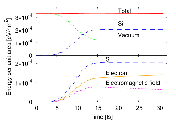
Figure 2: Energies per unit area integrated over macroscopic coordinate ${\mathrm{Z}}$ are shown as a function of time. In the upper panel, the energies integrated over ${\mathrm{Z}}<0$ (vacuum), ${\mathrm{Z}}>0$ (Si), and the whole region (Total) are compared. In the lower panel, the energy integrated over Si crystal region is decomposed into the field part and the electronic excitation part. The incident laser pulse is the same as that of Fig. 1.

In Fig. 2, we show energies per unit area integrated over the macroscopic coordinate. In the upper panel, the energy is decomposed into vacuum region (${\mathrm{Z}}<0$, green dotted line) and Si crystal region (${\mathrm{Z}}>0$, blue dashed line). The sum of the two contributions is shown by red solid line, showing that the total energy is well conserved during the whole period.

In the lower panel, the energy per unit area in the Si crystal region is decomposed into contributions of electronic excitations and electromagnetic fields. Since the electromagnetic fields are separated into reflected and transmitted fields after 15 fs, the energy of Si crystal region does not change in that period. The energy of transmitted electromagnetic fields decreases gradually as it is transferred to electronic excitation.

Figure 3: State of the system at $t=21$ fs after the peak of the incident pulse reaches the surface for several different intensities of the incident laser pulse. Left: the field divided by light speed, $A/c$; right: excitation energy per atom in the Si crystal.

We next show reflected and transmitted electromagnetic fields at different intensity levels. In the left panels of Fig. 3, the vector potentials are shown at a time when the transmitted and reflected waves are well separated. In the right panels, the electronic excitation energies per atom is shown in the Si crystal region. At the lowest intensity, the propagation of electromagnetic fields are well described by dielectric response. Essentially all of the energy remains associated with the propagating transmitted pulse. As the incident intensity increases, the transmitted wave becomes weaker than that expected from the linear response. We also find the central part of the transmitted pulse is suppressed strongly, producing a flat envelope of the pulse. In contrast, the envelope of the reflected wave does not change much in shape even at the highest intensity. We also find, at the intensity of $10^{13}$ W/cm², an emission of electromagnetic field is seen from the surface following the main pulse of reflected wave. From the right panels, above $10^{12}$ W/cm² one sees that most of the energy is deposited in the medium with just a small fraction remaining in the transmitted electromagnetic pulse. The deposition rate falls off with depth as to be expected from the weakening of the pulse. At higher intensities the absorption rate greatly increases. At $I_{0}=10^{13}$ W/cm² and higher the transmitted pulse is almost completely absorbed in the first tenths of a $\mu$m.

Figure 4: The reflectivity of Si at normal incidence is shown as a function of peak laser intensity.

In Fig. 4, we show the reflectivity as a function of incident laser intensity. Below $10^{12}$ W/cm², the reflectivity is constant and in accord with dielectric theory (Eq. (34)). Above $10^{12}$ W/cm², the reflectivity dips slightly, showing a minimum around $10^{13}$ W/cm². Above that intensity, the reflectivity start to increase gradually and finally reach 0.75 at the intensity of $5\times 10^{14}$ W/cm². This behavior of reflectivity qualitatively follows the observed evolution with intensity so00 , where it was interpreted in a dielectric model including effects of the excited electrons. We will later compare this model with our calculated reflectivity function.

IV.2 Excitation in surface layer

Figure 5: The vector potential divided by light speed (left panels) and electronic excitation energy (right panels) at the surface cell are shown as a function of time.

We next examine in more detail the first cell at the surface. The left-hand panel of Fig. 5 shows the vector potential as a function of time for several laser intensities. From a dielectric response, we expect the field inside the Si crystal is related to the incident field by $A_{t}=(2/1+\sqrt{\epsilon})A_{i}$. This relation holds well below $10^{12}$ W/cm². At higher intensities, the field is less than this estimate gives. We also observe an oscillation of the vector potential after the incident pulse ends at $10^{13}$ W/cm², in accordance with what we found in Fig. 3. We will later consider this phenomenon with a model dielectric function.

The electronic excitation energy in the first cell is shown in the right-hand panel of Fig. 5. At the lowest intensities, the electronic energy is carried by the transmitted wave and leaves the cell after passage of the pulse. As the laser intensity increases, energy is transferred irreversibly to electronic excitation, and reaches a plateau after the laser pulse has passed ($t>15$ fs). This is because the only mechanism to transfer energy between macroscopic grid points is through the macroscopic electromagnetic fields.

Figure 6: Excitation of the first layer of Si after the laser pulse ends. Excitation energy per Si atom (left panel) and density of electron-hole pairs as number of pair per Silicon atom (right panel) are shown as a function of laser intensity.

Figure 6 shows some final-state properties of the surface as a function of intensity. The residual excitation energy is shown in the left-hand panel. At low intensities, the energy deposited is proportional to $I_{0}^{2}$. This is the expected dependence for two-photon absorption. This is the most favorable absorption process in view of the photon energy: single-photon absorption is forbidden below the direct band gap, but the two-photon process is allowed. At $I_{0}\approx 10^{13}$ W/cm² the excitation energy is 0.6 eV per Si atom. This energy is in the form of electron-hole pairs. The minimum energy of a pair is at the direct band gap, 2.4 eV. However, the excitation process forms a coherent pair with energies distributed across the valence and conduction bands. In the TDDFT dynamics, the coherence is lost after the pulse moves on, but the energy distribution remains the same.

The number of particle-hole pairs $n_{ph}$ in the cell does not change after the electromagnetic field has passed. Then the number be calculated as the sum of overlaps of the time-dependent orbitals and the original Kohn-Sham orbitals,

$$n_{ph}=\sum_{i}\left\{1-\sum_{j}|\langle\psi_{j,{\mathrm{Z}}}(0)|\psi_{i,{\mathrm{Z}}}(t)\rangle|^{2}\right\},$$ (36)

where the sum over $i,j$ is taken over occupied orbitals. The results are shown in the right panel of Fig. 6.

Figure 7: Electronic excitation energy per electron-hole pair as a function of laser intensity.

As seen from the figure, the density increases quadratically with $I_{0}$ up to to a point and then continues to increase more gradually. The ratio of energy density to particle-hole pair density, shown in Fig. 7, has a simple interpretation. At low intensities, up to about $10^{12}$ W/cm², it coincides accurately with two-photon energy $2\hbar\omega_{\ell}=3.1$ eV. The energy per pair gradually increases at higher intensities. There one may expect two processes which increase the energy per pair. One is higher-order multiphoton absorption, as has been often discussed ke65 ; re80 . The other is the secondary excitation of electrons which have already been excited.

With the information about the particle-hole density $n_{ph}$, we may interpret the reflectivity curve (Fig. 4) with a model for the dielectric function that includes plasma effects. For example, in Ref. so00 and me10 , the response of electrons excited in conduction band is described with the Drude model. We consider the following simplified form for the dielectric function,

$$\varepsilon(\omega,n_{ph})=\varepsilon(\omega,0)-\frac{4\pi e^{2}n_{ph}}{m^{*}}\frac{1}{\omega\left(\omega+\frac{i}{\tau}\right)}\,.$$ (37)

Here $\varepsilon(\omega,0)$ is the dielectric function in the ground state; $m^{*}$ and $\tau$ are parameters of the Drude model. For our comparison we take $\varepsilon(\omega,0)$ from the linear response (see Appendix) at $\omega=\omega_{\ell}=1.55$ eV. The reflectivity associated with the model dielectric function is determined from Eq. (34).

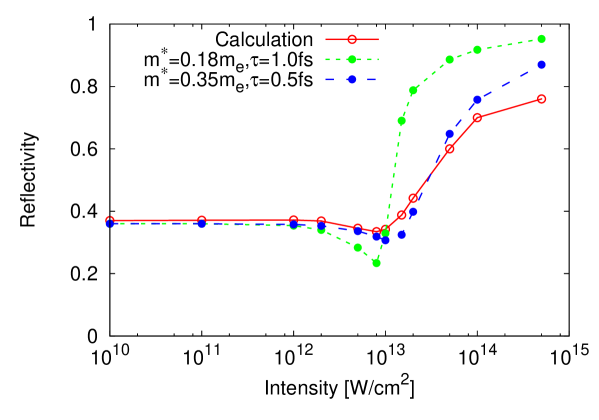
Figure 8: The reflectivity of Si at normal incidence is shown as a function of peak laser intensity. The red open circles with solid line repeat the calculated results from Fig. 4. The green filled circles with dotted line and blue filled circles with dashed line use Eqs. (34) and (37) with $m^{*}=0.18m$, $\tau=1.0$fs, and $m^{*}=0.35m$, $\tau=0.5$fs, respectively.

Figure 8 shows the comparison for two assumptions about the effective mass and Drude damping time. For a given laser intensity, we use the electron-hole density $n_{ph}$ in our calculation shown in Fig. 6. The red open circle with solid line is the present calculation. The green filled circle with dotted line is the effective mass and damping time adopted in Ref. so00 , $m^{*}=0.18m$ and $\tau=1$ fs. The blue filled circle with dashed line is the parameters adopted in Ref. me10 , $m^{*}=0.35m$ and $\tau=0.5$ fs. One can see that on a qualitative level, both the dip and the strong increase can be explained by plasma effects. One could try to fit the plasma parameters to reproduce the reflectivity curve, but it is probably not realistic to assume that a fixed dielectric function is responsible for the electromagnetic interactions. However, it should be mentioned that the reflectivity as well as the absolute value of the dielectric function are minimized when the screened plasma frequency,

$$\omega_{p}^{2}=\frac{4\pi e^{2}n_{ph}}{\epsilon(\omega_{\ell},0)m^{*}},$$ (38)

coincides with the frequency of the incident laser pulse, $\omega_{\ell}=\omega_{p}$. This relation is fulfilled at the laser intensity around $10^{13}$ W/cm², consistent with the behavior of reflectivity.

In Figs. 3 and 5, we observed an emission of electromagnetic field following the main pulse of the reflected wave at the laser intensity of $10^{13}$ W/cm². This phenomenon may also be understood with the model dielectric function. At this intensity, a small magnitude of the dielectric function at the surface allows a penetration of transmitted wave inside the medium. However, the dielectric function changes rapidly inside the medium due to the increase of electron-hole pair density. It may cause a reflection from a deeper layer, producing the electromagnetic field following the main pulse.

IV.3 Multi-scale vs single-cell approximations

In Ref. ot08 , we calculated microscopic electron dynamics for an external electric field normal to the crystal surface and neglecting magnetic fields. In this longitudinal geometry, the crystal response is uniform and the TDDFT is computationally much less expensive. This was applied to the dielectric breakdown for diamond crystal, and the calculated threshold for breakdown was at least an order of magnitude higher than the measured threshold.

The aim of the present subsection is twofold. First we show that the present multi-scale calculation gives much lower breakdown threshold than that of our previous calculation in the longitudinal geometry, thus resolving the discrepancy of our previous calculations with measurements. Second, we clarify mutual relationship between the present multi-scale calculation and the single-cell treatment in either the longitudinal or transverse geometry. Since the single-cell calculations are much easier computationally, it would be useful to know what physical information may be extracted reliably from them.

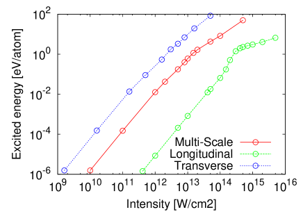
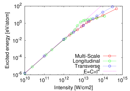
Figure 9: Deposited energy in the Si medium. Red solid line: the energy deposited in the first-layer in the multi-scale calculation. Green, dashed line: microscopic calculation in the longitudinal geometry. Blue dotted line: microscopic calculation in the transverse geometry. In the left panel, the horizontal axis is the intensity of the incident laser pulse for multi-scale calculation, and is the intensity of the applied laser pulses in the microscopic calculations of longitudinal and transverse geometries. In the right panel, the laser intensity is normalized to the transverse case. See the text for more detail.

We first explain in more detail the longitudinal and transverse geometries in the single-cell calculations. In the transverse geometry, we simply put the vector potential of applied laser pulse, $A(t)$, in the Kohn-Sham Hamiltonian and calculate the electron dynamics. In the longitudinal geometry, we take that field as external and add to it the field from the induced current in the medium. The vector potential in the Kohn-Sham Hamiltonian is the sum of the external and the induced fields, $A(t)=A_{ext}(t)+A_{ind}(t)$.

The final-state electronic excitation energies for the three calculations are shown in Fig. 9. In the left panel, the red circles and solid line shows the deposited energy at the surface in the multi-scale calculation as a function of the incident laser intensity. The green circles and dashed line is the microscopic calculation in the longitudinal geometry, as adopted in Ref. ot08 . The blue circles and dotted line is the microscopic calculation in the transverse geometry. We may identify the dielectric breakdown at the laser intensity where the electron excitation energy per atom is about 1 eV. One sees that the threshold for dielectric breakdown is very different for the three calculations. The threshold is lower by an order of magnitude for the multi-scale and transverse cases than the longitudinal case.

The difference may be understood using a dielectric picture to relate the internal and external fields. In the transverse case, the applied electric field directly acts upon electrons in the medium. In the case of the multi-scale calculation, the electric field in the medium and the incident field are related by

$${\cal E}_{medium}={2\over 1+\sqrt{\epsilon}}{\cal E}_{in}$$ (39)

Putting the value of dielectric constant $\epsilon=16$, the laser intensity is different between the transverse and multi-scale calculations by a factor of $(2/5)^{2}=0.16$. In the longitudinal case, in addition to the above factor connecting medium and incident fields, we need to add the following factor connecting the external and the medium fields,

$${\cal E}_{ext}=\epsilon{\cal E}_{medium},$$ (40)

The factor to correct the laser intensity is $16^{2}(2/5)^{2}=41$ for the longitudinal geometry. Taking these factors as corrections to the laser intensity, we replot the electronic excitation energy as a function of laser intensity in the medium in the right panel of Fig. 9. We see that these factors explain accurately the order-or-magnitude difference in the dielectric breakdown threshold. The electronic excitation energy coincides accurately below $10^{12}$ W/cm² for three calculations, where excitations are mostly by two-photon absorption. There are some deviations around $10^{13}$ W/cm² and above, where the resonant excitation is expected. The longitudinal calculation shows an abrupt rise of the excitation energy which we interpreted as a resonant energy transfer from the laser pulse to the electrons ot08 . The other two calculations do not produce an abrupt rise but rather show a smooth saturation of the energy transfer.

V Summary and outlook

We have developed a first-principles framework to calculation the propagation of electromagnetic field in crystalline solids. The macroscopic electromagnetic field is described by Maxwell equations while the microscopic electron dynamics is described by TDDFT. With use of massively parallel computers, we showed that it is feasible to treat one of the simplest systems of physical interest, the propagation of a laser pulse into bulk Si at the normal incidence.

At low field intensity, the calculated field propagation and electronic excitations exhibit features expected from ordinary electromagnetic theory with the dielectric function given by linear response theory. The electronic excitations are dominated by two-photon absorption at low intensities since the laser frequency is below the direct bandgap.

As the laser intensity increased, the density of excited electron-hole pairs become high enough to affect the response. This is conveniently modeled as an electron-hole plasma. At around $10^{13}$ W/cm², the plasma frequency of excited electrons reaches the visible frequency, showing a nonlinear interaction with the incident laser pulse. Above this intensity, the responses are dominated by nonlinear electron dynamics.

We have also found that the surface absorption obtained in the multi-scale theory can be described by a single-cell approximation using dielectric formulas to relate the internal and external fields, provided the fields do not much exceed $10^{13}$ W/cm².

Finally, we mention some directions that might be interesting to take up in later work. Analytic approximations have been proposed to express the excitation energy as a function of the Keldysh parameter ke65 . We have not examined the validity or accuracy of such approximations, but it would be useful to have this information.

Computations in the present framework could be extended to deal with laser pulses at oblique angles of incidence. In that case, the field is not translationally invariant in the $x$ direction, but the medium itself is. Consequently relatively few cells would be needed to describe the $x$ dependence. It would also be interesting to extend the present calculations to pump-probe laser pulse protocols. In principle it is straightforward to calculate the response to a double pulse separated in time. As a practical matter, pump-probe responses could most easily be studied in a single-cell approximation. Also, one could examine the linear response of the excited system using fields of the pump-probe form. This is important to verify the validity of the arguments made in Sect. IV.2.

Appendix

Here we show how the dielectric function may be calculated using the formalism of Sect. II.E. For the perturbation, we take $A$ to be of the form

$$A(t)=A_{0}\theta(t)\,.$$ (41)

The microscopic equation of motion Eq. (9) is integrated from $t=0$ to $t=T_{m}$ to obtain the $J(t)$ over the time interval. As is evident from Eq. (24), the calculated $J(t)$ is proportional to the conductivity as a function of time,

$$\sigma(t)=-\frac{c}{A_{0}}J(t).$$ (42)

This is Fourier transformed as

$$\sigma(\omega)=\int_{0}^{T_{m}}dt\,e^{i\omega t}f(t)\sigma(t)$$ (43)

where $f(t)$ is a filter to suppress spurious oscillations that would arise from a sharp cutoff of the integration at $T_{m}$. We employ a third order polynomial for it ya06 . The dielectric function may be obtained from the conductivity by Eq. (25).

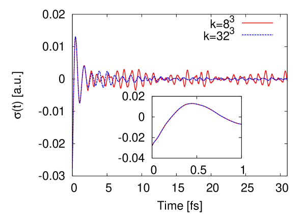
Figure 10: Conductivity as a function of time. Calculations for two choices of $k$-points are compared.

We carried out this computation taking $A_{0}=0.0005$ a.u. and $T_{m}=31$ fs (16,000 time steps with $\Delta t=0.08$ a.u.). In Fig. 10, we show a conductivity as a function of time, $\sigma(t)$, for two choices of $k$-points, $8^{3}$ and $32^{3}$. In our multi-scale calculation, we adopt $8^{3}$ $k$-points. Two calculations coincide each other up to 2 fs. There remain oscillations for a long period in the calculation of $8^{3}$ $k$-points, which are washed out if one employs a finer $k$-points grid.

Figure 11: Conductivity and dielectric function as a function of frequency in which $32^{3}$ $k$-points are used. The measured value is also shown for dielectric function.

The conductivity $\sigma(t)$ is Fourier transformed to obtain the conductivity and dielectric function as a function of frequency. They are shown in Fig. 11, in which $32^{3}$ $k$-points are used. At a frequency region close to zero, the conductivity $\sigma(\omega)$ should behave

$$\sigma(\omega)=i\left.\frac{d\sigma}{d\omega}\right|_{\omega=0}\omega.$$ (44)

In actual calculation, it is not exact due to the presence of spurious mode which originates from a violation of translational invariance in the real-space grid calculation. Since a small deviation from the above analytic behavior at around $\omega=0$ harms the low frequency behavior of the dielectric function, we replace the real part of the dielectric function by a second order polynomial of the frequency below 1 eV. The calculated dielectric function, $\epsilon(\omega)$, shown in the right panels of Fig. 11, is very close to the one calculated in Ref. sh10 using the formalism of Ref. be00 .

The calculated real part of the static dielectric function is $\epsilon(0)=12.6$, close to the experimental value of 11.6. However, as is well known in the density functional theory, the direct band gap in the local density approximation is smaller than the experimental one (2.4 eV theory vs. 3.1 eV experiment).

References

- (1) J.L. Krause, K.J. Schafer, and K.C. Kulander, Phys. Rev. A45, 4998 (1992).
- (2) S. Chelkowski, T. Zuo, and A.D. Bandrauk, Phys. Rev. A46, R5342 (1992).
- (3) I. Kawata, H. Kono, and Y. Fujimura, J. Chem. Phys. 110, 11152 (1999).
- (4) M. Petersilka and E.K.U. Gross, Laser Phys. 9, 105 (1999).
- (5) F. Calvayrac, P.-G. Reinhard, E. Suraud, and C.A. Ullrich, Phys. Rep. 337, 493 (2000).
- (6) X.-M. Tong and S.-I. Chu, Phys. Rev. A64, 013417 (2001).
- (7) K. Nobusada, K. Yabana, Phys. Rev. A70, 043411 (2004).
- (8) A. Castro, M.A.L. Marques, J.A. Alonso, G.F. Bertsch, and A. Rubio, Euro. Phys. J. D28, 211 (2004).
- (9) T. Otobe, M. Yamagiwa, J.-I. Iwata, K. Yabana, T. Nakatsukasa, and G.F. Bertsch, Phys. Rev. B77, 165104 (2008).
- (10) Y. Shinohara, K. Yabana, Y. Kawashita, J.-I. Iwata, T. Otobe, G.F. Bertsch, Phys. Rev. B82 155110 (2010).
- (11) Y. Miyamoto, H. Zhang, D. Tomanek, Phys. Rev. Lett. 104, 208302 (2010).
- (12) A. Fratalocchi and G. Ruocco, Phys. Rev. Lett. 106 105504 (2011).
- (13) T. Iwasa and K. Nobusada, Phys. Rev. A80, 043409 (2009).
- (14) T. Iwasa and K. Nobusada, Phys. Rev. A82, 043411 (2010).
- (15) H. Chen, J.M. McMahon, M.A. Ratner, and G.C. Schatz, J. Phys. Chem. C114, 14384 (2010).
- (16) E. Lorin, S. Chelkowski, and A. Bandrauk, Comp. Phys. Comm. 177, 908 (2007).
- (17) D.H. Reitze, H. Ahn, and M.C. Downer, Phys. Rev. B45, 2677 (1992).
- (18) D. von der Linde and H. Schüler, J. Opt. Soc. Am. B 13, 216 (1996).
- (19) M. Lenzner, J. Krüger, S. Sartania, Z. Cheng, Ch. Spielmann, G. Mourou, W. Kautek, and F. Krausz, Phys. Rev. Lett. 80, 4076 (1998).
- (20) K. Sokolowski-Tinten and D. von der Linde, Phys. Rev. B 61, 2643 (2000).
- (21) R. Huber, F. Tauser, A. Brodschelm, M. Bichler, G. Abstreiter, and A. Leitenstorfer, Nature 414, 286 (2001).
- (22) M. Nagai and M. Kuwata-Gonokami, J. Phys. Soc. Japan 71, 2276 (2002).
- (23) S.S. Mao, F. Quere, S. Guizard, X. Mao, R.E. Russo, G. Petite, P. Martin, Appl. Phys. A79, 1695 (2004).
- (24) D.M. Rayner, A. Naumov, and P.B. Corkum, Opt. Exp. 13, 3208 (2005).
- (25) H. Dachraoui and W. Husinsky, Phys. Rev. Lett. 97, 107601 (2006).
- (26) S.W. Winkler, I.M. Burakov, R. Stoian, N.M. Bulgakova, A. Husakou, A. Mermillod-Blondin, A. Rosenfeld, D. Ashkenasi, I.V. Hertel, Appl. Phys. A84, 413 (2006).
- (27) B. Rethfeld, Phys. Rev. Lett. 92, 187401 (2004).
- (28) J.R. Peñano, P. Sprangle, B. Hafizi, W. Manheimer, and A. Zigler, Phys. Rev. E72, 036412 (2005).
- (29) B. Rethfeld, Phys. Rev. B73, 035101 (2006).
- (30) L. Hallo, A. Bourgeade, V.T. Tikhonchuk, C. Mezel, and J. Breil, Phys. Rev. B76, 024101 (2007).
- (31) G.M. Petrov and J. Davis, J. Phys. B41, 025601 (2008).
- (32) N. Medvedev and B. Rethfield, J. Appl. Phys. 108, 103112 (2010).
- (33) T. Otobe, K. Yabana, and J.-I. Iwata, J. Phys. Cond. Matter 21, 064224 (2009).
- (34) G.F. Bertsch, J.-I. Iwata, A. Rubio, and K. Yabana, Phys. Rev. B 62 7998 (2000).
- (35) J.R. Chelikowsky, N. Troullier, K. Wu, and Y. Saad, Phys. Rev. B50, 11355 (1994).
- (36) K. Yabana and G.F. Bertsch, Phys. Rev. B54, 4484 (1996).
- (37) K. Yabana, T. Nakatsukasa, J.-I. Iwata, and G.F. Bertsch, phys. stat. sol. (b)243, 1121 (2006).
- (38) G.F. Bertsch and K. Yabana, Introduction to Computational Methods in Many Body Physics, Chap. 3 eds. M. Bonitz and D. Semkat, Rinton Press 2006.
- (39) J.P. Perdew and A. Zunger, Phys. Rev. B23, 5048 (1981).
- (40) N. Troullier and J.L. Martins, Phys. Rev. B43, 1993 (1991).
- (41) L.V. Keldysh, Soviet Physics JETP 20 1307 (1965); J. Exp. Tho. Phys (USSR) 47 1945 (1964).
- (42) H.R. Reiss, Phys. Rev. A 22 1786 (1980).