Particle correlation from uncorrelated non Born-Oppenheimer SCF wavefunctions

Abstract

We analyse a nonadiabatic self-consistent field method by means of an exactly-solvable model. The method is based on nuclear and electronic orbitals that are functions of the cartesian coordinates in the laboratory-fixed frame. The kinetic energy of the center of mass is subtracted from the molecular Hamiltonian operator in the variational process. The results for the simple model are remarkably accurate and show that the integration over the redundant cartesian coordinates leads to couplings among the internal ones.

1 Introduction

Typical quantum-mechanical treatments of molecular systems are based on the Born-Oppenheimer (BO) approximation that separates the motions of nuclei and electronsBJ00 . One first solves an eigenvalue equation for the electrons in the field of nuclei clamped at some predetermined points in space and thus builds the potential-energy surface (PES). Then one solves an equation for the nuclei moving on that PES and obtains the allowed energies of the molecule. In many cases the calculation is restricted to the neighborhood of the minimum of the PES in order to determine the molecular geometrySO96 . Accurate PES’s are useful for chemical-kinetic studiesF73 .

There has recently been great interest on the calculation of molecular properties by means of nonadiabatic approaches; i.e. without resorting to the BO approximation. Since the eigenfunctions of the Hamiltonian operator of the molecule $\hat{H}$ are not square integrable with respect to the $3N$ coordinates that describe the $N$ particles (electrons plus nuclei) in the laboratory-fixed coordinate axes one has to remove the unbounded motion of the molecular center of mass and the three corresponding coordinates. Thus one is left with the Schrödinger equation for the resulting molecular Hamiltonian operator in the molecule-fixed coordinate axes $H_{M}$ that depends on $3N-3$ coordinates and momenta. For brevity, from now on we call those coordinates absolute and relative (or internal), respectively. By means of the variational method one obtains an approximate eigenfunction of $H_{M}$ that should be also eigenfunction of the operators that commute with $H_{M}$, such as, for example, spin, angular momentum operator in relative coordinates, etcW91 ; FE10 .

There are several strategies for solving the Schrödinger equation without the BO approximation. One of them is based on explicitly correlated Gaussian functions of the relative coordinates of all the electrons and nuclei in the molecule (for a comprehensive review see Bubin et alBCA05 ). The trial function constructed from those Gaussians satisfies the permutational symmetry of identical particles and contains several parameters that are to be determined according to the variational method. If the Gaussians are located at one nuclei it is not difficult to choose the variational wavefunction to be eigenfunction of the angular-momentum operator. In some cases it is convenient to place the centers of the Gaussians on different space points and it is more difficult to force the variational function to be eigenfunction of the angular-momentum operator. In these calculations the authors explicitly expressed the variational function and the Hamiltonian operator in relative coordinatesBCA05 (and references therein).

Another widely spread strategy is based on uncorrelated functions and the SCF approach. In this case the variational function is written as a product of one-particle functions with the appropriate permutational symmetry. Since there are nuclear orbitals in addition to electronic ones this approach has been termed nuclear orbital plus molecular orbital (NOMO) theoryTMNI98 ; N02 ; NHM05 ; HN06 ; MHN06 ; N07 and also (but no longer in use now) dynamic extended molecular orbital (DEMO) methodTO00 . Since such orbitals are expressed in terms of the $3N$ absolute cartesian coordinates one has to be careful to avoid the spurious contribution of the kinetic energy of the center of massF10 . In order to avoid this problem Nakai et alNHM05 ; HN06 ; MHN06 ; N07 proposed to subtract the kinetic energy of the molecular center of mass from the Hamiltonian operator during the variational optimization of the trial wavefunction and developed the translation-free NOMO (TF-NOMO).

Although the NOMO approach is a nonadiabatic method its implementation is reminiscent of the BO approximation in that the orbitals are located at the “experimental geometries”NHM05 . Note that such a concept is rather alien to the nonadiabatic quantum-mechanical calculation just outlined (compare it with the more rigorous approach described by Bubin et alBCA05 ). The properly symmetrized product of orbitals located at different points and expressed in terms of absolute coordinates is not an eigenfunction of the angular-momentum operatorNHM05 ; HN06 ; MHN06 ; N07 . For that reason several rotational states are expected to contribute to the optimized variational function.

In order to remove the contribution of rotational states with angular-momentum quantum number $J>0$ Nakai et alNHM05 ; HN06 ; MHN06 ; N07 proposed a rotation-free NOMO that consists of subtracting also the rotational kinetic energy from the total Hamiltonian operator. The resulting approach is named translation- and rotation-free NOMO (TRF-NOMO). However, the removal of the spurious rotational kinetic energy in this way is not exact as in the case of the translation kinetic energy as argued by SutcliffeS05 .

The purpose of this paper is the analysis of the performance of the TF-NOMO and the effect of using absolute cartesian coordinates in the trial wavefunction. Since the treatment of realistic examples may be rather cumbersome we apply the method to a simple exactly solvable model.

In order to make this paper sufficiently self-contained, and to facilitate the discussion throughout, in Sec. 2 we outline the separation of the kinetic energy of the center of mass and the construction of the molecular Hamiltonian in relative coordinates. In Sec. 3 we apply the TF-NOMO to an exactly solvable model in order to test the accuracy of this approach and the effect of using the absolute coordinates instead of the internal ones. Finally, in Sec. 4 we discuss the results and draw conclusions.

2 Molecular Hamiltonian

In this section we outline some general properties of the nonrelativistic Hamiltonian operator for a system of $N$ charged point particles with only Coulomb interactions. The results are well known and have been discussed by several authors in different contexts (see, for example, the review by Fernández and EchaveFE10 and the references therein). The nonrelativistic Hamiltonian operator for a molecule can be written as

$$\hat{H} = \hat{T}+\hat{V},$$

$$\hat{T} = \sum_{i=1}^{N}\frac{\hat{p}_{i}^{2}}{2m_{i}},$$

$$V = \frac{1}{4\pi\epsilon_{0}}\sum_{i=1}^{N-1}\sum_{j=i+1}^{N}\frac{Q_{i}Q_{j}}{r_{ij}}$$ (1)

where $m_{i}$ is the mass of particle $i$, $Q_{i}=-e$ or $Q_{i}=Z_{i}e$ are the charges of either an electron or nucleus, respectively, and $r_{ij}=|\mathbf{r}_{i}-\mathbf{r}_{j}|$ is the distance between particles $i$ and $j$ located at the points $\mathbf{r}_{i}$ and $\mathbf{r}_{j}$, respectively, from the origin of the laboratory-fixed coordinate system. In the coordinate representation $\mathbf{\hat{p}}_{i}=-i\hbar\nabla_{i}$.

Since the the uniform translation of all the particles $\hat{U}(\mathbf{a})\mathbf{r}_{i}\hat{U}(\mathbf{a})^{\dagger}=\mathbf{r}_{i}+\mathbf{a}$ leaves the Coulomb potential invariant $\hat{U}(\mathbf{a})V\hat{U}(\mathbf{a})^{\dagger}=V$, then the eigenfunctions of the translation–invariant Hamiltonian operator (1) are not square integrable. For that reason we separate the motion of the center of mass and define translation-invariant internal coordinates by means of a linear transformation

$$\mathbf{r}_{j}^{\prime}=\sum_{i}t_{ji}\mathbf{r}_{i}$$ (2)

It is our purpose to keep the transformation (2) as general as possible so that it applies to a wide variety of nonadiabatic approaches. We arbitrarily choose $\mathbf{r}_{1}^{\prime}$ to be the coordinate of the center of mass

$$t_{1i}=\frac{m_{i}}{M},\;M=\sum_{i}m_{i}$$ (3)

and $\mathbf{r}_{j}^{\prime}$, $j>1$ the translational-invariant coordinates

$$\sum_{i}t_{ji}=0,\;j>1$$ (4)

Note that if the coefficients of the linear transformation (2) satisfy equations (3) and (4) then

$$\hat{U}(\mathbf{a})\mathbf{r}_{j}^{\prime}\hat{U}(\mathbf{a})^{\dagger}=\mathbf{r}_{j}^{\prime}+\mathbf{a}\delta_{j1}$$ (5)

The choice of the coefficients of the transformation (2) for the translational-invariant variables $\mathbf{r}_{j}^{\prime}$, $j>1$ is arbitrary as long as they satisfy Eq. (4) (for a more detailed discussion see FE10 ).

As a result of the change of variables, the total Hamiltonian operator reads

$$\hat{H} = -\frac{\hbar^{2}}{2M}\nabla_{1}^{\prime 2}+\hat{H}_{M}$$

$$\hat{H}_{M} = -\frac{\hbar^{2}}{2}\sum_{j>1}\sum_{k>1}\left(\sum_{i}\frac{t_{ji}t_{ki}}{m_{i}}\right)\nabla_{j}^{\prime}\nabla_{k}^{\prime}+\frac{1}{4\pi\epsilon_{0}}\sum_{i=1}^{N-1}\sum_{j=i+1}^{N}\frac{Q_{i}Q_{j}}{r_{ij}}$$ (6)

where $\hat{H}_{M}$ is the internal or molecular Hamiltonian operator. The explicit form of the interparticle distances $r_{ij}$ in terms of the new coordinates $r_{k}^{\prime}$ may be rather cumbersome in the general case but there are particular choices that are suitable for the calculation of the integrals necessary for the application of the variational methodFE10 ; BCA05 . The treatment of the simple model in Sec. 3 shows one of those particular transformations.

For future reference it is convenient to define the center of mass and relative kinetic-energy operators

$$\hat{T}_{CM} = -\frac{\hbar^{2}}{2M}\nabla_{1}^{\prime 2}$$ (7)

$$\hat{T}_{rel} = -\frac{\hbar^{2}}{2}\sum_{j>1}\sum_{k>1}\left(\sum_{i}\frac{t_{ji}t_{ki}}{m_{i}}\right)\nabla_{j}^{\prime}\nabla_{k}^{\prime}$$ (8)

respectively, so that $\hat{T}=\hat{T}_{CM}+\hat{T}_{rel}$, $\hat{H}_{M}=\hat{T}_{rel}+V$, and $\hat{H}=\hat{T}_{CM}+\hat{H}_{M}$.

The inverse transformation $\mathbf{t}^{-1}$ exists and gives us the old coordinates in terms of the new ones:

$$\mathbf{r}_{i}=\sum_{j}\left(\mathbf{t}^{-1}\right)_{ij}\mathbf{r}_{j}^{\prime}$$ (9)

According to equations (5) and (9) we have $\hat{U}(\mathbf{a})\mathbf{r}_{i}\hat{U}(\mathbf{a})^{\dagger}=\left(\mathbf{t}^{-1}\right)_{i1}\mathbf{a}+\mathbf{r}_{i}$ from which we conclude that

$$\left(\mathbf{t}^{-1}\right)_{i1}=1,\;i=1,2,\ldots,N$$ (10)

In order to understand the meaning of this result note that the momentum conjugate to $\mathbf{r}_{i}^{\prime}$ is given by the transformation

$$\mathbf{\hat{p}}_{i}^{\prime}=\sum_{j}\left(\mathbf{t}^{-1}\right)_{ji}\mathbf{\hat{p}}_{j}$$ (11)

so that the linear momentum of the center of mass

$$\mathbf{\hat{p}}_{1}^{\prime}=\sum_{j}\mathbf{\hat{p}}_{j}$$ (12)

is precisely the total linear momentum of the molecule. We also appreciate that

$$T_{CM}=\frac{\mathbf{\hat{p}}_{1}^{\prime}\cdot\mathbf{\hat{p}}_{1}^{\prime}}{2M}=\frac{1}{2M}\sum_{i=1}^{N}\sum_{j=1}^{N}\mathbf{\hat{p}}_{i}\cdot\mathbf{\hat{p}}_{j}$$ (13)

The eigenfunctions of the total Hamiltonian operator (1) are of the form

$$\Psi(\mathbf{r}_{1},\ldots,\mathbf{r}_{N})=e^{i\mathbf{k}\cdot\mathbf{r}_{1}^{\prime}}\psi(\mathbf{r}_{2}^{\prime},\ldots,\mathbf{r}_{N}^{\prime})$$ (14)

with the appropriate permutational symmetry for the electrons and nuclei. We are of course interested in the wavefunction for the internal degrees of freedom $\psi(\mathbf{r}_{2}^{\prime},\ldots,\mathbf{r}_{N}^{\prime})$ that provides the relevant molecular properties. For this reason we should use a trial function of the corresponding coordinates $\varphi(\mathbf{r}_{2}^{\prime},\ldots,\mathbf{r}_{N}^{\prime})$ and apply the variational method with the relative or molecular Hamiltonian operator $\hat{H}_{M}$BCA05 .

Nakai et alNHM05 ; HN06 ; MHN06 ; N07 proposed an alternative route based on a trial function of the absolute cartesian coordinates $\varphi(\mathbf{r}_{1},\ldots,\mathbf{r}_{N})$ and applied the variational method to

$$W=\frac{\left\langle\varphi\right|\hat{H}-\hat{T}_{CM}\left|\varphi\right\rangle}{\left\langle\varphi\right|\left.\varphi\right\rangle}$$ (15)

More precisely, they resorted to the Hartree-Fock method with electronic and nuclear orbitals. In this equation one integrates with respect to $d\mathbf{r}_{1}d\mathbf{r}_{2}\ldots d\mathbf{r}_{N}$ (including spin if necessary) and the trial function $\varphi(\mathbf{r}_{1},\ldots,\mathbf{r}_{N})$ is square integrable with respect to all those $3N$ electronic and nuclear variables. This approach is called TF-NOMO method and is an improvement over the translation-contaminated NOMO TC-NOMO method (like, for example, the DEMOTO00 ) that is based on the variational method for $\hat{H}$. Note that the domain of the NOMO trial function $\varphi(\mathbf{r}_{1},\ldots,\mathbf{r}_{N})$ is $R^{3N}$ and that for the molecular wavefunction $\psi(\mathbf{r}_{2}^{\prime},\ldots,\mathbf{r}_{N}^{\prime})$ is $R^{3N-3}$. Thus, from a quantum-mechanical point of view they belong to different state spaces.

If we rewrite the arguments of the trial function in terms of internal coordinates $\varphi(\mathbf{r}_{1},\ldots,\mathbf{r}_{N})=\tilde{\varphi}(\mathbf{r}_{1},\mathbf{r}_{2}^{\prime},\ldots,\mathbf{r}_{N}^{\prime})$ then we appreciate that the probability distribution of the internal variables

$$\rho(\mathbf{r}_{2}^{\prime},\ldots,\mathbf{r}_{N}^{\prime})=\int\tilde{\varphi}(\mathbf{r}_{1},\mathbf{r}_{2}^{\prime},\ldots,\mathbf{r}_{N}^{\prime})^{2}\,d\mathbf{r}_{1}$$ (16)

may exhibit some degree of correlation even though the trial function $\varphi(\mathbf{r}_{1},\ldots,\mathbf{r}_{N})$ is merely a product of nuclear and electronic orbitals with the appropriate permutational symmetryNHM05 ; HN06 ; MHN06 ; N07 . The analysis of the effect of this particle correlation in a realistic molecular system appears to be rather complicated; for this reason in what follows we resort to a quite simple example.

3 Simple model

In order to have a clearer understanding of the TF-NOMO methodNHM05 ; HN06 ; MHN06 ; N07 we apply it to a simple exactly-solvable model. We are only interested in the removal of the translational contamination because getting rid of the rotational one does not appear to be so simpleS05 . Therefore, a one–dimensional model with at least three particles and a translation-invariant potential will suffice. Our model consists of three particles of masses $M_{1}$, $M_{2}$ and $M_{3}$ that move in one dimension and interact through forces that follow Hooke’s law:

$$\hat{H} = -\frac{\hbar^{2}}{2M_{1}}\frac{\partial^{2}}{\partial X_{1}^{2}}-\frac{\hbar^{2}}{2M_{2}}\frac{\partial^{2}}{\partial X_{2}^{2}}-\frac{\hbar^{2}}{2M_{3}}\frac{\partial^{2}}{\partial X_{3}^{2}}$$ (18)

$$+\frac{1}{2}\left[K_{12}\left(X_{1}-X_{2}\right)^{2}+K_{13}\left(X_{1}-X_{3}\right)^{2}+K_{23}\left(X_{2}-X_{3}\right)^{2}\right]$$

where $K_{ij}$ are the force constants.

In order to reduce the number of parameters to a minimum we first assume that the three particles are identical, so that $M_{1}=M_{2}=M_{3}=M$ and $K_{12}=K_{13}=K_{23}=K$. We define dimensionless coordinates $x_{i}=X_{i}/L$, where $L=\hbar/(m\omega)$ and $\omega=\sqrt{K/M}$ and obtain the dimensionless Hamiltonian

$$\hat{H}_{d} = \frac{\hat{H}}{\hbar\omega}=-\frac{1}{2}\left(\frac{\partial^{2}}{\partial x_{1}^{2}}+\frac{\partial^{2}}{\partial x_{2}^{2}}+\frac{\partial^{2}}{\partial x_{3}^{2}}\right)$$ (19)

$$+\frac{1}{2}\left[\left(x_{1}-x_{2}\right)^{2}+\left(x_{1}-x_{3}\right)^{2}+\left(x_{2}-x_{3}\right)^{2}\right]$$

and the dimensionless energy $\epsilon=E/(\hbar\omega)$.

We separate the motion of the center of mass by means of the transformation

$$q_{1} = \frac{1}{3}\left(x_{1}+x_{2}+x_{3}\right)$$

$$q_{2} = x_{2}-x_{1}$$

$$q_{3} = x_{3}-x_{1}$$ (20)

where $q_{1}$ is the coordinate of the center of mass and $q_{2}$ and $q_{3}$ are the coordinates of particles 2 and 3 with respect to the coordinate origin located arbitrarily at particle 1. These $q_{j}$’s are the $\mathbf{r}_{j}^{\prime}$’s of Sec. 2 and the transformation (20) satisfies the equations discussed there. We thus obtain

$$\hat{H}_{d}=\hat{T}_{CM}+\hat{H}_{r}$$ (21)

that is the sum of the dimensionless kinetic energy of the center of mass $\hat{T}_{CM}$ and the dimensionless Hamiltonian operator for the relative motion $\hat{H}_{r}$ ($\hat{H}_{M}$ in the general discussion of Sec. 2)

$$\hat{T}_{CM} = -\frac{1}{6}\frac{\partial^{2}}{\partial q_{1}^{2}}$$

$$\hat{H}_{r} = -\frac{\partial^{2}}{\partial q_{2}^{2}}-\frac{\partial^{2}}{\partial q_{3}^{2}}-\frac{\partial^{2}}{\partial q_{2}\partial q_{3}}+q_{2}^{2}+q_{3}^{2}-q_{2}q_{3}$$ (22)

The eigenfunctions are of the form

$$\Psi(q_{1},q_{2},q_{3})=e^{ikq_{1}}\psi(q_{1},q_{2})$$ (23)

where $\psi(q_{1},q_{2})$ is an eigenfunction of $\hat{H}_{r}$ and $-\infty<k<\infty$. Note that $\Psi(q_{1},q_{2},q_{3})$ is not square integrable with respect to $dx_{1}dx_{2}dx_{3}$ as expected from the fact that the motion of the center of mass is unbounded. The total dimensionless energy is $\epsilon_{T}=\epsilon+k^{2}/6$, where $\epsilon$ is the dimensionless energy of the relative motion (an eigenvalue of $\hat{H}_{r}$).

If we try the correlated gaussian function
$\varphi(q_{2},q_{3})=\left[\left(4a^{2}-b^{2}\right)/\pi^{2}\right]^{1/4}\exp\left[-a\left(q_{2}^{2}+q_{3}^{2}\right)-bq_{2}q_{3}\right]$,
where $4a^{2}-b^{2}>0$, then we obtain the exact ground-state eigenfunction of $\hat{H}_{r}$

$$\psi_{00}(q_{2},q_{3})=\frac{1}{\sqrt{\pi}}\exp\left[-\frac{\sqrt{3}}{3}\left(q_{2}^{2}-q_{2}q_{3}+q_{3}^{2}\right)\right]$$ (24)

with dimensionless energy $\epsilon_{00}=\sqrt{3}$.

As uncorrelated variational function in the absolute coordinates we try

$$\varphi(x_{1},x_{2},x_{3})=\left(\frac{2a}{\pi}\right)^{3/4}\exp\left[-a\left(x_{1}^{2}+x_{2}^{2}+x_{3}^{2}\right)\right]$$ (25)

that is square integrable with respect to $dx_{1}dx_{2}dx_{3}$. Note that there is a redundant coordinate because we need just two variables to describe the bound states of this model as shown in Eq. (24). This trial function is our simple version of a NOMO one. The optimal value of the variational parameter $a$ is determined by the minimum of

$$W(a)=\left\langle\hat{H}-\hat{T}_{CM}\right\rangle$$ (26)

as proposed by Nakai et alNHM05 ; HN06 ; MHN06 ; N07 , where

$$\hat{T}_{CM}=-\frac{1}{6}\left(\frac{\partial^{2}}{\partial x_{1}^{2}}+\frac{\partial^{2}}{\partial x_{2}^{2}}+\frac{\partial^{2}}{\partial x_{3}^{2}}+2\frac{\partial^{2}}{\partial x_{1}\partial x_{2}}+2\frac{\partial^{2}}{\partial x_{1}\partial x_{3}}+2\frac{\partial^{2}}{\partial x_{2}\partial x_{3}}\right)$$ (27)

is the kinetic-energy operator for the center of mass in the absolute coordinates. Note that present $\hat{T}_{CM}$ is what Nakai et alNHM05 call $\hat{T}_{T}$ and approximate by $\hat{T}_{n,T}$ in their calculations, and present approach is the straightforward application of the TF-NOMO to a simple one-dimensional model.

At first sight it is surprising that the variational function with the optimal value $a=\sqrt{3}/2$ of the adjustable parameter yields the exact energy $W(\sqrt{3}/2)=\sqrt{3}$. However, it is not the only striking fact because the expectation values of any function of $x_{2}-x_{1}$ and $x_{3}-x_{1}$ (like, for example, $(x_{2}-x_{1})^{2}$, $(x_{2}-x_{1})^{4}$, $(x_{2}-x_{1})(x_{3}-x_{1})$, etc) are exact too. In spite of this remarkable agreement the exact and approximate wavefunctions are not the same as follows from the fact that $\hat{T}_{CM}\psi_{00}=0$ and $\left\langle\varphi|\hat{T}_{CM}|\varphi\right\rangle=\sqrt{3}/4$. We will explain these curious results later on; for the time being note that the results of Nakai et alNHM05 for $E_{tot}^{TRC}-E_{tot}^{TF}=\left\langle\Phi_{0}\right|\hat{T}_{n,T}\left|\Phi_{0}\right\rangle\approx\left\langle\Phi_{0}\right|\hat{T}_{T}\left|\Phi_{0}\right\rangle$ yield the spurious contribution of the kinetic energy of the center of mass to the molecular energy. They state that this problem is due to the fact that the Gaussian functions are unsuitable for describing the translational energy but it is clear that a set of Gaussian functions in relative coordinates will not exhibit such undesirable behavior. In other words, the translational contamination is a consequence of adopting the absolute coordinates and not a result of the choice of Gaussian functions. The same argument applies to the rotational contamination; Bubin et alBCA05 show how to obtain Gaussian states with zero angular-momentum quantum number ($J=0$).

We may suspect that the unexpected success of the variational approach is partly due to the symmetry of the problem (three identical particles). In order to break it with the slightest modification of our model we choose $K_{12}=K_{13}=K\neq K_{23}$ and define $\lambda=K_{23}/K$, so that

$$\hat{H}_{d} = -\frac{1}{2}\left(\frac{\partial^{2}}{\partial x_{1}^{2}}+\frac{\partial^{2}}{\partial x_{2}^{2}}+\frac{\partial^{2}}{\partial x_{3}^{2}}\right)$$ (28)

$$+\frac{1}{2}\left[\left(x_{1}-x_{2}\right)^{2}+\left(x_{1}-x_{3}\right)^{2}+\lambda\left(x_{2}-x_{3}\right)^{2}\right]$$

and

$$\hat{H}_{r}=-\frac{\partial^{2}}{\partial q_{2}^{2}}-\frac{\partial^{2}}{\partial q_{3}^{2}}-\frac{\partial^{2}}{\partial q_{2}\partial q_{3}}+\frac{1}{2}\left[q_{2}^{2}+q_{3}^{2}+\lambda(q_{2}-q_{3})^{2}\right]$$ (29)

Since the masses remain the same the transformation from absolute to relative coordinates and the form of $T_{CM}$ are still given by equations (20) and (27), respectively.

The exact ground-state wavefunction and energy are given by

$$\psi_{00}(q_{2},q_{3}) = \frac{\left(4a^{2}-b^{2}\right)^{1/4}}{\sqrt{\pi}}\exp\left[-a\left(q_{2}^{2}+q_{3}^{2}\right)+bq_{2}q_{3}\right]$$

$$a = \frac{\sqrt{6}\left(\sqrt{6\lambda+3}+3\lambda+2\right)\sqrt{3\lambda+2-\sqrt{6\lambda+3}}}{12\left(3\lambda+1\right)}$$

$$b = \frac{\sqrt{6}\sqrt{3\lambda+2-\sqrt{6\lambda+3}}}{6}$$ (30)

and

$$\epsilon_{00}=\frac{\sqrt{2}\left(2\sqrt{2\lambda+1}+\sqrt{3}\left(\lambda+1\right)\right)\sqrt{3\lambda+2-\sqrt{6\lambda+3}}}{2\left(3\lambda+1\right)}$$ (31)

respectively.

As in the preceding example we consider an uncorrelated NOMO-like trial function of the absolute coordinates

$$\varphi(x_{1},x_{2},x_{3})=\frac{2^{3/4}\sqrt{b}a^{1/4}}{\pi^{3/4}}\exp\left[-ax_{1}^{2}-b(x_{2}^{2}+x_{3}^{2})\right]$$ (32)

where the optimal values of $a$ and $b$ minimize $W(a,b)=\left\langle\hat{H}_{d}-\hat{T}_{CM}\right\rangle$. In this case we have the following TF-NOMO parameters and energy

$$a = \frac{\sqrt{3}}{2},\;b=\frac{\sqrt{6(\lambda+1)}}{4}$$

$$W(a,b) = \frac{\sqrt{6(\lambda+1)}}{3}+\frac{\sqrt{3}}{3}$$ (33)

In order to measure the effect of keeping the kinetic energy of the center of mass we also choose the values of the variational parameters from the minimum of $W(a,b)=\left\langle\hat{H}_{d}\right\rangle$, which yields

$$a = \frac{\sqrt{2}}{2}$$

$$b = \frac{\sqrt{\lambda+1}}{2}$$

$$W(a,b) = \sqrt{\lambda+1}+\frac{\sqrt{2}}{2}$$ (34)

From now on we refer to equations (33) and (34) as TF-NOMO and TC-NOMO in order to make a connection with the approach of Nakai et alNHM05 .

Fig. 1 shows the exact and approximate dimensionless ground-state energy calculated in the two ways just outlined. As expected, TF-NOMO yields considerably more accurate results because TC-NOMO is strongly contaminated with the kinetic energy of the center of mass. This point was discussed earlier by FernándezF10 with respect to the DEMO methodTO00 . Note that TF-NOMO is remarkably accurate for all $\lambda$ and yields the exact result for $\lambda=1$ as discussed above.

We may try and improve the TC-NOMO results by simply subtracting the kinetic energy of the center of mass, thus producing a sort of corrected TC-NOMO or CTC-NOMO:

$$W^{CTCNOMO}=\left\langle\varphi^{TCNOMO}\right|\hat{H}_{d}-\hat{T}_{CM}\left|\varphi^{TCNOMO}\right\rangle$$ (35)

Figure 1 shows that the energy calculated in this way agrees quite well with the exact and TF-NOMO ones. This result shows that most of the error in the energy calculated by means of the TC-NOMO comes from the spurious kinetic energy and just a relatively small contribution comes from the inadequate optimization of the variational wavefunction with respect to $\hat{H}_{d}$.

It is not difficult to explain why the uncorrelated trial function in absolute coordinates yields such good results (even exact ones for $\lambda=1$). It we substitute $x_{2}=q_{2}+x_{1}$ and $x_{3}=q_{3}+x_{1}$ into equation (32) and integrate the square of $\tilde{\varphi}(x_{1},q_{2},q_{3})=\varphi(x_{1},q_{2}+x_{1},q_{3}+x_{1})$, with respect to $x_{1}$, we obtain

$$\rho(q_{2},q_{3})=\int_{-\infty}^{\infty}\tilde{\varphi}(x_{1},q_{2},q_{3})^{2}\,dx_{1}=\frac{2\sqrt{a}b}{\pi\sqrt{a+2b}}\exp\left[-\frac{2c\left(a+b\right)}{a+2b}\left(q_{2}^{2}+q_{3}^{2}\right)+\frac{4b^{2}q_{2}q_{3}}{a+2b}\right]$$ (36)

Note that the use of the absolute coordinates in the trial wavefunction introduces some sort of correlation between the translation-invariant coordinates $q_{2}$ and $q_{3}$ when we integrate with respect to the redundant variable. The resulting correlation is reasonable because it is determined by the variational method, and, in particular, when $\lambda=1$ it yields (fortuitously) the exact probability distribution for the relative coordinates

$$\rho(q_{2},q_{3})=\frac{1}{\pi}\exp\left[-\frac{2}{\sqrt{3}}\left(q_{2}^{2}+q_{3}^{2}-q_{2}q_{3}\right)\right]=\psi_{00}(q_{2},q_{3})^{2}$$ (37)

It is now clear why we obtained the exact energy and expectation values before for this particular case. In fact, we expect to obtain the exact expectation values of any observable in relative coordinates. We do not obtain the exact expectation value of $\hat{T}_{CM}$ because this operator contains a derivative with respect to the redundant absolute variable that does not appear in the exact square-integrable wavefunction.

In order to compare the approximate and exact wavefunctions we write both $\rho(q_{2},q_{3})$ and $\psi_{00}(q_{2},q_{3})^{2}$ as $\left[\left(4\alpha^{2}-\beta^{2}\right)^{1/2}/(2\pi)\right]\exp\left[-\alpha\left(q_{2}^{2}+q_{3}^{2}\right)+\beta q_{2}q_{3}\right]$ ($2\alpha>|\beta|$). Figures 2 and 3 show that the exponential coefficients $\alpha$ and $\beta$, respectively, given by the TF-NOMO agree remarkably well with the exact ones, whereas the TC-NOMO coefficients are considerably less accurate. Note that the effect of keeping the kinetic energy of the center of mass not only affects the energy (which is expected) but also the form of the variational wavefunction. The agreement between the exact and TF-NOMO exponential parameters $\alpha$ and $\beta$ explains why the approximate wavefunction yields so accurate expectation values of operators in the relative coordinates $q_{2}$ and $q_{3}$. In particular, the TF-NOMO results are exact for $\lambda=1$, but, of course, such a result is not to be expected in a realistic case.

If we minimize $\left\langle\varphi\right|\hat{H}_{r}\left|\varphi\right\rangle$ with an uncorrelated trial function of the relative coordinates

$$\varphi(q_{2},q_{3})=\sqrt{\frac{2a}{\pi}}\exp\left[-a(q_{2}^{2}+q_{3}^{2})\right]$$ (38)

we obtain the optimal variational parameter $a=\sqrt{2\lambda+2}/4$ and the resulting approximate energy $W(a)=\sqrt{2\lambda+2}$ is considerably less accurate than that given by Eq. (33). This result suggests that it is preferable to apply the NOMO method with orbitals that depend on the absolute coordinates as long as we remove the kinetic energy of the center of mass in the optimization process. That is to say, we minimize the expectation value of $\hat{H}_{r}=\hat{H}-\hat{T}_{CM}$ expressed, for simplicity, in the same set of absolute coordinates chosen for the NOMO variational wavefunction. Under such conditions the TF-NOMO-SCF method appears to take into account part of the correlation energy that in the present simple model is given by $W(a,b)-W(a)$. This energy difference is quite similar for TF-NOMO and CTC-NOMO according to Fig. 1.

4 Conclusions

We have tried to elucidate the effect of using absolute coordinates in the NOMO-SCF variational method. Since such an analysis for an actual molecule, even as simple as $H_{2}$, is rather complicated we chose a simple model of three particles with harmonic interactions in one dimension. Although rather oversimplified, this model enables us to take into account the main ingredients of the NOMO-SCF method. We have a translation-invariant potential-energy function and, consequently, we have to remove the unbounded motion of the center of mass. In this case a correlated Gaussian function of the relative coordinates yields the exact result that is most convenient to test the approximate ones.

The NOMO-SCF wavefunction is simply a product of Gaussian functions (orbitals) for each of the particles. The integration of the square this uncorrelated function with respect to the redundant absolute coordinate (three in a realistic case as shown in Eq. (16)) gives rise to some kind of particle correlation. If the adjustable parameters in this trial function are optimized variationally with the Hamiltonian $\hat{H}_{r}=\hat{H}-\hat{T}_{CM}$ then the correlation just mentioned appears to improve the calculation of the energy and expectation values considerably. Perhaps, one should not expect such a remarkable success for an actual molecule, but, however, there is no doubt that even in that case the NOMO-SCF will take into account part of the correlation energy in spite of being based on uncorrelated Gaussian functions. In order to verify this conjecture that is expressed in Eq. (16) it is only necessary to calculate the energy with an uncorrelated NOMO trial function and $\hat{H}_{r}$ both in terms of relative coordinates (like present Eq. (38)). Note that this interesting feature of the TF-NOMO has apparently passed unnoticed in the applications of the methodNHM05 ; HN06 ; MHN06 ; N07 . This fact reinforces our claim on the utility of simple models for the study of rather complicated problems.

The simple model also shows that if we simply subtract the expectation value of the kinetic energy of the center of mass then the resulting energy is quite accurate (what we have called CTC-NOMO). However, in order to improve the calculation of the expectation values of other observables it is convenient to apply the SCF procedure with the relative Hamiltonian operator $\hat{H}_{r}=\hat{H}-\hat{T}_{CM}$ that leads to what is commonly known as TF-NOMONHM05 ; HN06 ; MHN06 ; N07 .

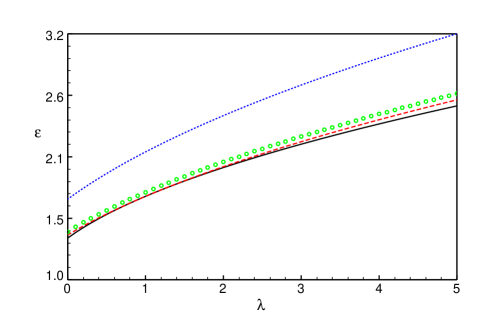
Figure 1: Exact (solid line, black), TF-NOMO (dashed line, red), TC-NOMO (points, blue) and CTC-NOMO (circles, green) ground–state dimensionless energy

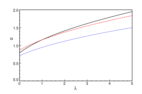
Figure 2: Exact (solid line, black), TF-NOMO (dashed line, red) and TC-NOMO (points, blue) exponential coefficient $\alpha$

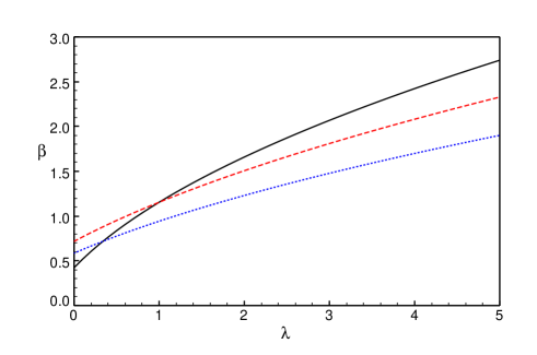
Figure 3: Exact (solid line, black), TF-NOMO (dashed line, red) and TC-NOMO (points, blue) exponential coefficient $\beta$

References

- (1) P. R. Bunker and P. Jensen, The Born-Oppenheimer Approximation, in: P. R. Bunker and P. Jensen (Ed.), Computational Molecular Spectroscopy, Vol. John Wiley & Sons, LTD, Chichester, New York, Weinheim, Brisbane, Toronto, Singapore, 2000).
- (2) A. Szabo and N. S. Ostlund, Modern Quantum Chemitrsy, (Dover Publications, Inc., Mineola, New York, 1996).
- (3) W. Forst, Theory of Unimolecular Reactions, (Academic Press, New York, London, 1973).
- (4) R. G. Woolley, J. Mol. Struct. (Theochem) 230, 17 (1991).
- (5) F. M. Fernández and J. Echave, Nonadiabatic Calculation of Dipole Moments, in: J. Grunenberg (Ed.), Computational Spectroscopy. Methods, Experiments and Applications, Vol. Wiley-VCH, Weinheim, 2010).
- (6) S. Bubin, M. Cafiero, and L. Adamowicz, Adv. Chem. Phys. 131, 377 (2005).
- (7) M. Tachikawa, K. Mori, H. Nakai, and K. Iguchi, Chem. Phys. Lett. 290, 437 (1998).
- (8) H. Nakai, Int. J. Quantum Chem. 86, 511 (2002).
- (9) M. Hoshino and H. Nakai, J. Chem. Phys. 124, 194110 (2006).
- (10) K. Miyamoto, M. Hoshimo, and H. Nakai, J. Chem. Theory Comput. 2, 1544 (2006).
- (11) H. Nakai, Int. J. Quantum Chem. 107, 2849 (2007).
- (12) H. Nakai, M. Hoshimo, and K. Miyamoto, J. Chem. Phys. 122, 164101 (2005).
- (13) M. Tachikawa and Y. Osamura, Theor. Chem. Acc. 104, 29 (2000).
- (14) F. M. Fernández, J. Phys. B 43, 025101 (2010).
- (15) B. Sutcliffe, J. Chem. Phys. 123, 237101 (2005).