Standard Model CP and Baryon Number Violation in Cold Electroweak Cosmology

Abstract

Contrary to popular beliefs, it is possible to explain Baryonic asymmetry of the Universe inside the Standard Model, provided inflation ended into a broken phase below the electroweak transition. Two important ingredients of the solution are multiquanta ”Higgs bags”, containing W,Z and top quarks, as well as sphaleron transitions happening inside these bags. Together, they provide baryon number violation at the level $10^{-2..3}$. Our recent calculations show that CP violation (due to the usual CKM matrix of quark masses in the 4-th order) leads to top-antitop population difference in these bags of about $10^{-9}$. (The numbers mentioned are not yet optimized and simply follow a choice made by some numerical simulations of the bosonic fields we used as a reference point.)

1 Cold electroweak scenario

It is a great honor to give a talk at this inaugural meeting of the Kobayashi-Maskawa Institute. Moreover, this invitation came at the moment whet I can report new exciting applications of the celebrated CKM matrix, to its originally intended purpose – explaining (perhaps) the most important CP-odd effect in our Universe, its baryonic asymmetry.

The question how it was produced is among the most difficult open questions of physics and cosmology. The observed effect is usually expressed as the ratio of the baryon density to that of the photons $n_{B}/n_{\gamma}\sim 10^{-10}$. Sakharov [1] had formulated three famous necessary conditions: the (i) baryon number and (ii) the CP violation, with (iii) obligatory deviations from the stationary ensembles such as the thermal equilibrium. Although all of them are present in the Standard Model (SM) and standard Big Bang cosmology, the baryon asymmetry which is produced by known CKM matrix is completely insufficient to solve this puzzle.

Significant efforts has been made to solve it using hypothetical “beyond the standard model” scenarios. In particular, possible large CP violating processes in the neutrino or in the supersymmetric sectors are possible. Although there are interesting proposals along those lines, they remain orders of magnitude away from feasible experimental tests.

An alternative we will discuss is the modification of the standard cosmology. The standard Big Bang scenario predicts adiabatically slow crossing of the electroweak phase transition, leading to extremely small deviations from equilibrium. The so called “hybrid” or “cold” scenario [2, 3, 4, 5] solve this difficulty by combining the end of the inflation era with the establishment of the electroweak broken phase. Since there is no space here to discuss it in detail, let me simply enumerate the main points of the emerging scenario: only few new points will be elaborated below.

• Large deviations from equilibrium, $O(1)$, with strongly oscillating Higgs and other fields [6, 7, 8, 9].
  

• Formation of relatively long-lived “hot spots” inside which the Higgs VEV is small [6, 7, 8, 9].
  

• Topologically nontrivial fluctuations of the gauge field lead to baryon number violation [6, 7, 8, 9] at overall level of $O(10^{-3})$
  

• These transitions take place only $inside$ the “hot spots” [6, 7, 8, 9].
  

• The first nonscalar quanta produced are those with large mass (that is, stronger coupled to Higgs), namely the top quarks/antiquarks and the gauge bosons [17].
  

• Tops and gauge bosons are collected into the “hot spots”, which are then mechanically balanced. These objects are identified [17] with the (non-topological) solitons called the W-Z-top bags found independently[18]
  

• Baryon number violation events are identified with Carter-Ostrovsky-Shuryak (COS) sphalerons with the size tuned to those of the hot spots
  

• The B violation processes, described by the well known 12-fermion ’t Hooft operator, can occure as various subprocesses, $n\rightarrow 12-n,n=0..12$ . The most probable was argued [17] to be the “top recycling $\bar{t}\bar{t}\bar{t}\rightarrow 9$ which is converting the energy of the tops or antitops already present in the bag into that of the gauge field, which helps passing high barrier separating different topologies
  

• If so, the asymmetry of top and anti-top populations in the bag leads to different production rate of the baryon and antibaryon numbers [10]
  

• Clear “time arrow” of the process is given by the fact that a top quark, after a weak decay into lighter quarks, simply diffuse away from the bag since all quarks lighter than the top cannot be bound to the bag [10]
  

• The usual CKM mechanism of the CP violation naturally produces the top-antitop asymmetry via interferences of various outgoing paths of these light quarks, in the 4-th order in weak interaction [10]
  

2 The multi-quark bags

Being a scalar, the Higgs generates universal attraction between all kinds of particles. Furthermore, the strength of the attraction is proportional to their total mass, similar to the gravity interacting with the total energy. Gravity, feeble as it is, holds together planets, stars and even create black holes. Unlike vector forces induced by electric, weak or color charges, gravity and scalar exchanges are exempt from “screening” and thus their weak coupling can be compensated by a large number $N$ of participating particles. And yet, unlike gravity, the Higgs boson is neither massless, nor even particularly light in comparison to $W,Z$ or $t$. So, are there multi-quanta states based on the Higgs attraction?

Another instructive analogy is provided by the nuclear physics. Think of a (much-simplified) Walecka model, in which the nuclear forces can be approximately described by the $\sigma$, “the Higgs boson of the nuclear physics”, and $\omega$ meson exchanges. Because of similarity of masses $m_{\sigma}\sim 600\,MeV,m_{\omega}\sim 770\,MeV$, as well as couplings, the sigma-induced attraction is nearly exactly canceled by the omega-induced repulsion. Their sum is an order of magnitude smaller than one would get from scalar and vector components taken separately.

Can the situation at electroweak scale similar? Perhaps the Standard Model is just a low energy effective Lagrangian, hiding some deeper physics behind its simplistic scalar Higgs. We are not aware of any particular model which suggests a vector companion to Higgs with a similarly small mass $O(100\,GeV)$ mass. For example, the “techni-$\rho$” is predicted to be at the scale $M_{\rho}\sim 1\,TeV$. Thus, unlike in the nuclear physics, one is $not$ expecting the scalar-vector cancellation.

The interest in the issue of “top bags” originated from the question whether a sufficiently heavy SM-type fermion should actually exist as a bag state, depleting the Higgs VEV around itself. Although classically this seemed to be possible, it was shown in refs [11, 12, 13] that quantum (one loop) effects destabilize such bags, except at so large coupling at which the Yukawa theory itself becomes apparently sick, with an instability of its ground state. The issue rest dormant for some time till Nielsen and Froggatt [14] suggested to look at the first magic number, 12 tops+antitops corresponding to the maximal occupancy of the lowest $l=0,\,j=1/2$ orbital, with 3 colors and 2 from $t+\bar{t}$. Using simple formulae from atomic physics these authors suggested that such system forms a deeply-bound state. In ref.[15] we have checked this claim and found that, unfortunately, this is $not$ the case. While for a massless Higgs there are indeed weakly bound states of 12 tops, they disappear way below the realistic Higgs mass. Further variational improvement of the binding conditions for the 12-quark system [16] confirmed that 12 tops are unbound for Higgs mass $m_{H}>M_{c}(12)\sim 50\,GeV$.

Assuming spherical symmetry, the Higgs energy reads

$$E_{Higgs}=2\pi v^{2}\int_{0}^{\infty}dr\,r^{2}\left[\phi^{\prime\,2}+\frac{1}{4}\,m_{H}^{2}\,(\phi^{2}-1)^{2}\right]$$ (1)

where $v=246\,GeV$ ,$m_{H}^{2}\equiv 2\lambda v^{2}$ is the Higgs mass, taken to be a round number $m_{H}=100\,GeV$ in the original papers (we also use units of $100\,GeV$ throughout this paper). Consider now the addition of a conserved (during the time scale we are interested in) $N$ particles (fermions or bosons), couple strongly to the Higgs field which could be strongly distorted. We adopt a mean-field approximation, in which all the particles are described by the same wave functions in the background of the Higgs field. Corrections to this mean-field description, such as, many-body, recoil and retardation of the Higgs field are expected to be suppressed by factors $v/m$, $m_{H}/m$ and $1/N$. In the semiclassical approximation, the total energy of the system will be given by $E_{cl}=E_{Higgs}+\sum_{a}n_{a}\varepsilon_{a},$ where $\{\varepsilon_{a}\}$ is the spectrum of the corresponding field in the Higgs background, $n_{a}$ is the occupation number of each state and $N=\sum_{a}n_{a}$ is the total, conserved, particle number.

In the Higgs vacuum, i.e. $\phi(r)=1$, the state of lowest energy with $N$ particles has total energy $NM$. However, in the background of a non-trivial Higgs field there are two competing effects. On the one hand, the gradient and potential terms increase the energy but, on the other hand, there might be some bound states levels with energy $0<\varepsilon_{a}<M$ which can allocate the quanta, lowering the energy of the system of particles at the expense of creating such distortion.

Let us start by a crude estimate of the the order of magnitude of $N$ for which such bags may exist. If we were to deplete a certain large volume of the Higgs VEV (surface/kinetic terms neglected for now), it would require an energy $V_{bag}\frac{m_{H}^{2}}{8}v^{2}$. For a bag of radius, say, $R\cdot 100\,GeV$=4, this energy is about 20 $TeV$. Thus, if the lowest W-boson energy level has a binding energy of the order of $30\,GeV$ per $W$ or $Z$, an order of $O(1000)$ of them would be needed to compensate for the bag energy and obtain some binding. The top quarks are heavier and may get much larger binding, so one might naively think that less of them would suffice: but Pauli exclusion principle makes it more delicate.

Consider the propagation of $W$-bosons in an external Higgs field

$$\left(\Box+M_{W}^{2}\phi^{2}\right)W^{\mu}+\partial^{\mu}\left(\frac{W^{\nu}\partial_{\nu}\phi^{2}}{\phi^{2}}\right)=0.~{}~{}\quad$$ (2)

Let us study these equations of motion in the usual electric (e), longitudinal (l) and magnetic (m) basis $\boldsymbol{W}^{(e,l,m)}=\boldsymbol{Y}^{(e,l,m)}_{jm}f_{(e,l,m)}(r)/r,$ where $\boldsymbol{Y}_{jm}$ are spherical harmonic vectors and $f_{e}(r),f_{l}(r)$ and $f_{m}(r)$ are the radial wave functions for each mode. In a static, spherically symmetric, background the last term in (2) vanishes for the magnetic mode, leading to the simple Klein-Gordon equation: but in this case $j\geq 1$. For others one can start with smaller $j=0$ without a centrifugal potential, but the Laplacian mixes the electro-longitudinal modes, leading to the set of coupled equations (see the original paper) in which the last term in (2) becomes large and positive in the region where the Higgs field $\phi$ approaches zero, effectively repelling the longitudinal modes from the bag. (Note that massless gauge fields have no longitudinal degree of freedom at all.) As a consequence, even $j=0$ mode is pushed above that $j=1$ magnetic modes, which is thus the lowest. In order to find bag solutions for finite $N$, we adopted a variational approach and took as a trial function for the Higgs, e.g. the Gaussian profile

$$\phi(r)=1-\alpha\,\exp{(-r^{2}/w^{2})},$$ (3)

with two parameters, $\alpha$ and $w$ describing its depth and the width, respectively. Solving the W-boson magnetic equation in this Higgs background is rather straightforward

In Fig. 1(a) we show some results for a bag with $\alpha=1.3$. It is now relatively simple thing to vary the shape and reach the minimum of the energy of the system (still in the spherically symmetric ansatz.)

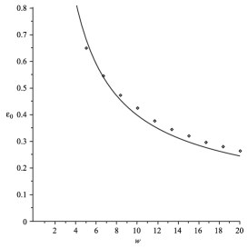
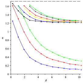
Figure 1: (a) The energy of the lowest magnetic mode ($j=1$) $E/(100\,GeV$ for a Gaussian bag with $\alpha=1.3$ versus its width. The numerical results (points) are in good accordance with the analytical result, see [18]. (b) Dependence of fermionic bound state levels energy $\varepsilon$ in units of $100\,GeV$ on the size of the bag, expressed as the parameter $R$ in units $1/100\,GeV^{-1}$ for a bag with $\eta=1$. The color coding of the levels and their quantum numbers are listed in Table I.

Now we consider a system of $N$ heavy fermions interacting with a background Higgs field, the standard notations for Dirac spinors in spherical coordinates are

$$\psi=\frac{1}{r}\left(\begin{array}[]{c}F(r)\Omega_{jlm}\\ (-1)^{1/2(1+l-l^{\prime})}G(r)\Omega_{jl^{\prime}m}\end{array}\right),$$ (4)

where $\Omega_{jlm}$ are spherical 2-component spinors and we take normalization $\int dr\,(F^{2}+G^{2})=1$. The so-called Dirac parameter $\kappa$ is defined as

$$\kappa=\left\{\begin{array}[]{c}-(l+1)\text{ \ \ \ for }j=l+1/2\\ l\text{ \ \ \ \ \ \ \ \ \ \ \ \ \ \ for\ }j=l-1/2\end{array}\right.$$ (5)

and runs over all nonzero integers, being positive for anti-parallel spin and negative for parallel spin. The Dirac’s equation reads

$$(\varepsilon-m\,\phi)\,F~{}\, = \,-G^{\prime}\,+\,(\kappa/r)\,G$$ (6)

$$(\varepsilon+m\,\phi)\,G~{}\, = \,\,~{}~{}F^{\prime}\,+\,(\kappa/r)\ F$$

The form of these equations presumes that the eigenvalue $\varepsilon$ is positive. A negative eigenvalue would correspond to a state in the lower fermion continuum. If so, a charge conjugation transformation turns it into a positive eigenvalue for an antifermion. The Higgs equation of motion reads

$$\phi^{\prime\prime}+\frac{2}{r}\phi^{\prime}+\frac{m_{H}^{2}}{2}\phi\,(1-\phi^{2})\,=\,\frac{(N-1)m}{4\pi\,v^{2}}\,\frac{F^{2}-G^{2}}{r^{2}}$$ (7)

Note that in the $r\rightarrow\infty$ limit, the source term in the right hand side, as well as the additional $\phi^{\prime}/r$ term from the Laplacian can be neglected and the equation becomes the usual equation for a 1D kink.

The spectrum for Dirac’s equation is found numerically and examples of the levels are shown in Fig.1. The Table shows magic numbers and the order in which levels are populated. Some levels are also shown in Fig. 1.

	$n_{r}$	$\kappa$	$l$	$j$	$Deg.(\bar{t}t)$	color
1	0	-1	0	1/2	12	blue
2	0	-2	1	3/2	24	red
3	0	-3	2	5/2	36	green
4	0	1	1	1/2	12	black

Table 1: The properties of some levels, including the number of radial nodes $n_{r}$, Dirac parameter $\kappa$, orbital momentum $l$, total angular momentum $j$, multiplicity of states $Deg$(for $t\bar{t}$ bags) and color code used in our figures.

Attempting to find a minimum of the total energy, tops and Higgs, we have found that the ratio of the top-to-Hoggs masses are simply not large enough to stabilize bags by themselves. So tops can only exist inside the W-bags. Free (or weakly bound) top quarks are much heavier than $W$ bosons and thus decay into another quark and the $W$. In the Higgs bag, however, we found that two lowest top levels are below the lowest gauge boson ones; so up to 36 $t+\bar{t}$ in such bags may live much longer, given by next order decays into three fermions, like in the usual beta decays.

3 The sphalerons and rates

In the broken phase the electroweak sphalerons had been found by Manton et al: their mass is about 14 TeV and thus the tunneling rate is prohibitively small. In pure gauge sector finding the sphaleron solution has been precluded by the fact that classical gauge theory has no scale and thus energy has no minimum. It has been surpassed in [19] by requiring minimization under two conditions: fixed Chern-Symons number and mean-square radius $\rho$.

The profile of the the magnetic field in COS configuration is given by the following spherically symmetric expression

$$B^{2}(r)={48\rho^{4}\over g^{2}(r^{2}+\rho^{2})^{4}}$$ (8)

This form does indeed fit well the numerically found shapes of the $B^{2}$ at the “sphaleron moment”, a maximum of magnetic field. Fitted radius, yielding $m\rho\approx 3.9$ which corresponds to the total energy of the COS sphaleron

$$E_{tot}=3\pi^{2}/g^{2}\rho\approx 2\,\,TeV$$ (9)

which is 7 times less than the KM sphaleron mass: it makes a huge difference for he rate.

Combining all the factors we find that numerical value of preexponent and exponent nearly cancels out, leaving crudely

$$\Gamma/Vm^{4}\sim 10^{-1}$$ (10)

with accuracy say an order of magnitude or so. With that accuracy it agrees with the results of the simulations which also finds that the number of sphaleron transitions per spot is indeed about several percents.

What should happen after the sphaleron moment? Sphaleron decay is a classical downhill rolling of the classical (high amplitude) gauge field, from the (sphaleron) top into the next classical vacuum . This process was extensively studied numerically for the broken-phase sphaleron. Remarkably, an $analytic$ solution of the time-dependent explosion of COS sphaleron has also been found in the COS paper [19]. The late time profile of the energy density of the expanding “empty” shell.

$$4\pi\epsilon(r,t)={8\pi\over g^{2}\rho^{2}r^{2}}\left({1\over 1+(r-t)^{2}/\rho^{2}}\right)^{3}$$ (11)

Comparing the explosion of COS sphaleron with numerical data one can see both the similarities and the differences between them. Indeed, there is an empty shell formation at some time. However the inside of the shell does not remain empty: in fact the topology and magnetic field have a secondary peak (of smaller magnitude). Qualitatively it is easy to see why it happens. The COS sphaleron is a solution exploding in zero Higgs background, with massless gauge fields at infinity. In the numerical simulations we discuss such explosion happens inside the finite-size cavity. As the gauge bosons of the expanding shell hit the walls of the no-Higgs spot, they are massive outside. With some probability they

Since the original numerical simulations have included the gauge fields but ignored fermions, we have to discuss first, at quite qualitative level, what their effects can be, relative to that of the gauge fields. Those tops would be added to the metastable bubbles of the symmetric phase, the no-Higgs spots, like the W discussed above.

The well known Adler-Bell-Jackiw anomaly require that a change in gauge field topology by $\Delta Q\pm 1$ must be accompanied by a corresponding change in baryon and lepton numbers, B and L. More specifically, such topologically nontrivial fluctuation can thus be viewed as a “t’Hooft operator” with 12 fermionic legs. Particular fermions depend on orientation of the gauge fields in the electroweak SU(2): since we are interested in utilization of top quarks, we will assume it to be “up”. In such case the produced set contains $t_{r}t_{b}t_{g}c_{r}c_{b}c_{g}u_{r}u_{b}u_{g}\tau\mu,e$ , where $r,b,g$ are quark colors. to which we refer below as the $0\rightarrow 12$ reaction. Of course, in matter with a nonzero fermion density many more reactions of the type $n\rightarrow(12-n)$ are allowed, with $n$ (anti)fermions captured from the initial state.

The classical solution describing the expansion stage at $t>0$ has been worked out for COS sphaleron explosion, and for the “compression stage” at $t<0$ one can use the same solution with a time reversed. At very early time or very late times $t\rightarrow\pm\infty$ the classical field become weak and describe convergent/divergent spherical waves, which are nothing but certain number of colliding gauge bosons. Fermions of the theory should also be treated accordingly. Large semiclassical parameter – sphaleron energy over temperature – parametrically leads to the assumption that total bosonic energy is much larger than that of the fermions, so one usually ignores backreaction and consider Dirac eqn for fermions in a given gauge background. For KM sphaleron and effective $T$ we discuss, this parameter would be $\sim 70$, which is indeed large compared to 12 fermions. However in the case of COS sphaleron we are going to use the number is about $\sim 10$, comparable to the number of fermions produced. It implies that backreaction from fermions to bosons is very important.

The only (analytic) solution to Dirac eqn of the “expansion stage” was obtained in [20], it describes motion from the COS sphaleron zero mode (at $t=0$) all the way to large $t\rightarrow+\infty$ physical outgoing fermions, with analytically calculated momentum distribution. A new element pointed out in [17] is that its time-reflection can also describe the “compression stage”, in which free fermions with the $negative$ energy are captured by a convergent spherical wave of gauge field at $t\rightarrow-\infty$, ending at the zero energy sphaleron zero mode at $t=0$.

This implies that energy of the initial fermions can be incorporated and used in the sphaleron transition. The optimum way to generate sphaleron transition turns out to be 3 initial top quarks considering the $3\rightarrow 9$ fermion process instead of the original $0\rightarrow 12$ one. The $3\rightarrow 9$ fermion process saves a lot of energy, as in it the initial top quark energy can be completely transferred from the “sphaleron doorway state” to the gauge field. Estimates show that it increases the sphaleron rate by about one order of magnitude, compared to pure gauge calculation.

4 The CP asymmetry

The first attempts to estimate magnitude of CP violation in cold electroweak cosmology has been made by Smit, Tranberg and collaborators [21, 8]. Their strategy has been to derive some local effective CP-odd Lagrangian by integrating out quarks, and than include this Lagrangian in their real-time bosonic numerical simulations. The estimated magnitude of the CP-odd effects ranges from $n_{B}/n_{\gamma}\sim 10^{-6}..10^{-10}$ [9], which reignites hopes that this scenario can provide the observed magnitude of the baryon asymmetry in Universe. However, there are many unanswered questions about the accuracy of these estimates. One of them [17] is that the effective Lagrangian derived with specific scale of the loop momenta, e.g. $p\sim m_{c}$, can only be used for field configurations at a scale softer than this loop scale: and the “hot spots” in numerical simulations obviously do not fit this condition. But in practice even more important is the following unanswered generic question: why should a very complicated operator (containing 4-epsilon symbol convoluted with 4 gauge field potentials and one field strength) averaged over very complicated field configurations (obtained only numerically) have $nonzero$ average at all? We were thinking about some model fields (e.g. sphalerons) in which these operators have nonzero values, but were not able to find any convincing examples. Since the calculation is numerical, it would be desirable to have some parametric estimate of the effect, in particular to know what sign the effect should have and at least some bound on it from below. These goals are reached in the last paper [10].

For a top quark starting at the position $r_{1}$, the escaping amplitude has the form

$$A_{t}(r_{1})=\int\gamma^{\nu}W^{-}_{\nu}V^{\dagger}P_{t}S_{d}^{L}(r_{1},r_{2})\gamma^{\mu}W^{+}_{\mu}VS_{u}^{L}(r_{2},r_{c})d^{4}r_{2},$$ (12)

whereas the anti-top has a C-reflected expression

$$A_{\bar{t}}(r_{1})=\int\gamma^{\nu}W^{+}_{\nu}\bar{V^{\dagger}}P_{\bar{t}}S_{d}^{L}(r_{1},r_{2})\gamma^{\mu}W^{-}_{\mu}\bar{V}S_{u}^{L}(r_{2},r_{c})d^{4}r_{2}.$$ (13)

Here $V$ is the CKM matrix, $S$ the quark propagators, their index $u,d$ etc denotes the up and/or down quark flavors and $P_{t}$ denote the flavor matrix making the initial projection on the top quark.

The probablility of a top quark escaping from $r_{1}$ is then given by the integral over all positions and sum over all intermediate and final states $f$ of the squared amplitude

$$Prob_{t}(r_{1}) = \int_{f}A_{t}^{\dagger}A_{t}=Tr\int d^{4}r_{c}\sum_{u}A_{t}^{\dagger}A_{t}=\int d^{4}r_{c}d^{4}r_{2}d^{4}r_{3}Tr\left[P_{t}\gamma^{\nu}W^{-}_{\nu}V^{\dagger}S_{d}^{L}(r_{1},r_{2})\right.$$

$$\gamma^{\mu}W^{+}_{\mu}VS_{u}^{L}(r_{2},r_{c})S_{u}^{L\dagger}(r_{c},r_{3})\left.\gamma^{\alpha}W^{-}_{\alpha}V^{\dagger}S_{d}^{L\dagger}(r_{3},r_{1})\gamma^{\beta}W^{+}_{\beta}V\right].$$

Note that the interference terms between different paths are of the 4-th order in weak interaction, and thus have 4 CKM matrices, as indeed is needed for the CP violation effects. Four positions of the points at which the interactions take place, as well as particular quark flavor in the intermediate line, are summed over. Writing the amplitude squared of the process, one includes the unitarity cut (the vertical line in Fig.2) to the right of which one, as usual, finds the conjugated image of the process in opposite direction.

In between these four points the flavor of the quark remains unchanged. Quark wave functions (we keep in mind $l=0$ or $s$-wave ones only, thus points are only indicated by their radial distance from the bag) are different for each flavor, because of different Yukawa couplings to Higgs profile. Semiclassically the phase is approximated

$$S_{12}=exp[i\int_{r_{1}}^{r_{2}}p(x)dx]\approx exp[i\int_{r_{1}}^{r_{2}}(E-{\frac{m_{i}^{2}(x)}{2E}})dx],$$ (14)

where $E$ is the quark energy, and the approximation implies that all lower quark flavors are light in respect to $r/E$, so that the flavor-dependent phase (stemming from the second term in the bracket) is still smaller than 1

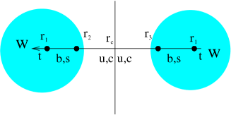
Figure 2: (Color online) Schematic shape of the 4 order process involving only quarks of the 2nd and 3ed generations. The shaded objects on the left and right represent the Higgs bag with strong gauge fields (indicated by W in the figure) inside. The vertical line is the unitarity cut. Four black dots indicate 4 points, indicated with $r_{i},i=1..4$ where $W$ quanta are interacting with the quark, changing it from upper ($t$=top) to lower ($b,s$) components.

Let us follow the flavor part of the amplitude, which distinguishes between quarks and anti-quarks. The 4-th order process we outlined in the preceeding section corresponds to the trace of the following matrix product

$$M_{t}=Tr(P_{t}*V*S_{12}^{down}*V^{+}*S^{up}_{23}*V*S^{down}_{31}*V^{+}),$$ (15)

where $S$ are quark propagators, the lower indices specify their initial and final points, the upper subscript remind us that those are for up or down quark components. $P_{t}$ is the projector requiring that we start (and end the loop) in the bag, with a top quark. We also define the amplitude for the top-antiquarks

$$M_{\bar{t}}=Tr(P_{t}*V^{*}*S_{12}^{down}*V^{T}*S^{up}_{23}*V^{*}*S^{down}_{31}*V^{T})$$ (16)

which we subtract from $M_{t}$, as the effect we evaluate is the difference in the top-antitop population inside the bag. The difference gets CP-odd as seen from its dependence on the CP-odd phase $\delta$

$$M_{t}-M_{\bar{t}}=2iJ(S^{u}_{23}-S^{c}_{23})(-S^{s}_{31}*S^{b}_{12}-S^{d}_{31}*S^{s}_{12}+S^{d}_{31}*S^{b}_{12}$$

$$+S^{d}_{12}*S^{s}_{31}-S^{d}_{12}*S^{b}_{31}+S^{s}_{12}*S^{b}_{31})$$ (17)

$$J=\sin(\delta)\sin(\theta_{12})\sin(\theta_{13})\sin(\theta_{23}\cos(\theta_{23})\cos(\theta_{12})\cos^{2}(\theta_{13})\cos(\theta_{23})$$

The remaining combination of propagators, organized in two brackets, needs to be studied fiurther. Note first that the propagators in the range 2-3 (through the unitarity cut) factor out and that one may ignore the top quarks there. Note further, that if the $u,c$ quarks would have the same mass, the first bracket would vanish: this is in agreement with general arguments that any degenerate quarks should always nullify the CP-odd effects, as the CP odd phase can be rotated away already in the CKM matrix itself.

The last bracket in (17) contains interferences of different down quark species: note that there are 6 terms, 3 with plus and 3 with minus. Each propagator, as already noticed in the preceeding section, has only small corrections coming from the quark masses. Large terms which are flavor-independent always cancel out, in both brackets in the expression above. Let us look at only the terms which contain the heaviest $b$ quark in the last bracket, using the propagators in the form $S^{q}_{ij}\sim exp\left(\pm i\frac{m_{b}^{2}}{2E}r_{ij}\right)$ where $\pm$ refers to different signs in the amplitude and conjugated amplitude and $r_{ij}=r_{j}-r_{i}$. Note that the sign of the phase between points $r_{2}$ and $r_{3}$ can be positive or negative as it results from a subtraction of the positive phase from $r_{3}$ to the cut $r_{c}$ with the negative phase form the cut $r_{c}$ to $r_{2}$. Terms containing odd powers in $r_{23}$ therefore should vanish in the integral: and the lowest term we have is quadratic. Considering all phases to be small due to $1/E$ and using the mass hierarchy $m_{b}\gg m_{s}\gg m_{d}$ we pick up the leading contribution of the last bracket in (17) which has $r_{23}^{2}$ and the 4-th power in the last bracket, the 6-th order in the phase shift in total:

$$M_{t}-M_{\bar{t}}\propto J\frac{m_{b}^{4}m_{c}^{4}m_{s}^{2}r_{23}^{2}r_{12}r_{31}(r_{12}+r_{31})}{64E^{5}}.$$ (18)

Note that all distances in this expression are defined to be positive and the sign in the last bracket is plus, so unlike all the previous orders in the phase expansion, at this order we have sign-definite answer with no more cancellations possible. This point is the central one in this work. We further see that this expression grows for large $r$’s, which are to be integrated over. Of course as we expanded the exponent in the phases, they have to be such that these phases are smaller than 1.

Let us start with a “naive” estimate, which assumes that $E$ in the formulae is given by the top quark mass $E\sim m_{t}=173\,GeV$. As for the field strength, naively one may take all four interaction points inside the bags, where the amplitude of the $W$ is the strongest. If so, all distances $r_{ij}$ are of the order of the bag size $R_{bag}\sim 1/m_{W}$. However, if this is the case, all the phases are so small that the resulting CP asymmetry is about 10 orders of magnitude smaller than needed. However, the initial top quarks are bound in the bag, so light quarks can be propagating at the energy much smaller than the top mass. The smallest possible scale is fixed by the weak interaction of quarks with the electroweak plasma outside the bag, known as the screening mass $\sim g_{w}T$, which is few GeV. This is the natural scale to take: thus we will from now consider $E\sim m_{b}$ in the following. Another improvement one may try is to consider locations of some points $outside$ the bag, selecting $r_{ij}$ as large as possible.

$$Prob_{t-\bar{t}}(r_{1}) \sim J\frac{m_{b}^{4}m_{c}^{4}m_{s}^{2}}{64E^{5}}\int dr_{2}dr_{3}2r_{2}r_{3}^{2}f(r_{1})^{2}f(r_{2})f(r_{3}).$$ (19)

Considering a radial bag of $N_{W}$ weak bosons having an exponential profile with the usual $W$ mass in the broken phase: $W(r)=\sqrt{\frac{N_{w}m_{w}^{3}}{\pi E_{w}}}e^{-m_{w}r},$ we get that the probability of a top-minus-antitop quark escaping

$$\delta_{CP}=\tau JN_{w}^{2}\frac{m_{c}}{16E}\frac{m_{b}^{4}}{E^{4}}\frac{m_{c}^{3}}{m_{w}^{3}}\frac{m_{s}^{2}}{E_{w}^{2}}\sim 10^{-10}\left(\frac{N_{w}}{1000}\right)^{2}.$$ (20)

In the latter formula we made use of the lifetime of the bag denoted $\tau/m_{W}$, with $\tau\sim 6$ to bound the time integral over $x_{1}$.

The main lesson we got from this study is that the scales of both the quark energy $E$ and their traveling distances $r_{ij}$ in the loop amplitudes should be tuned individually, to maximize the effect. The main limitation come from the conditions of quark rescattering in the plasma (the screaning masses) and the conditions that all phases $\delta_{i}$ should not be large, as well as the limitations coming from the $W$ field strength and correlation length. Another lesson is that in order to prevent cancellations between different flavors, one has to expand all the results till sign-definite answer is guaranteed.

The probability to find 3 antitops is actually proportionnal to $(1+\delta_{CP})^{3}\approx 1+3\delta_{CP}$, while it is $(1-3\delta_{CP})$ for tops: it gives factor 3. Another factor 3 appears because of the fact that each sphaleron event creates 3 units of baryon number, not one. Together with baryon asymmetry (time integrated) sphaleron rates of $10^{-2}$ and $3*3*\delta_{CP}$ we arrive to our final estimate $\Delta B\sim 10^{-11\pm 1}$ where one order of magnitude stands for our (perhaps optimistic) errors due to numerical factors ignored in the estimates. We conclude that it is clearly in the same ballpark as the observed baryonic asymmetry of the Universe. Clearly, numerical factors can be detailed later, and the parameters of the cosmological model can be better tuned to get closer the right value.

Last but not least is the issue of the $sign$ of the asymmetry. Our formula (18) has definite (positive) sign, that is to say more top quark escape the bag (note that the time direction is important, quarks are first created in the bag, then have more probability to escape). More antitops remain in the bags, with more likely to be “recycled” by the sphalerons: this produces more baryons than anti-baryons. Apparently we got the right sign for the baryon asymmetry.

Acknowledgements I just was lucky to get invited and give a talk: all it contains I learned with my collaborators over the years. I should also acknowledge very useful recent discussion of these issues with J.Smit and A.Tranberg.

References

- [1] A. D. Sakharov, JETP Lett. 6, 24 (1967).
- [2] J. García-Bellido, D. Grigoriev, A. Kusenko and M. Shaposhnikov, Phys. Rev. D 60, 123504 (1999).
- [3] L. M. Krauss and M. Trodden, Phys. Rev. Lett. 83, 1502 (1999).
- [4] G. N. Felder, J. Garcia-Bellido, P. B. Greene, L. Kofman, A. D. Linde and I. Tkachev, Phys. Rev. Lett. 87, 011601 (2001) [arXiv:hep-ph/0012142].
- [5] J. Garcia-Bellido, M. Garcia Perez and A. Gonzalez-Arroyo, Phys. Rev. D 67, 103501 (2003) [arXiv:hep-ph/0208228].
- [6] J. Garcia-Bellido, M. Garcia-Perez and A. Gonzalez-Arroyo, Phys. Rev. D 69, 023504 (2004) [arXiv:hep-ph/0304285].
- [7] A. Tranberg and J. Smit, JHEP 0311, 016 (2003) [arXiv:hep-ph/0310342].
- [8] A. Tranberg, A. Hernandez, T. Konstandin, M. G. Schmidt, Phys. Lett. B690 (2010) 207-212. [arXiv:0909.4199 [hep-ph]].
- [9] A. Tranberg, [arXiv:1009.2358 [hep-ph]].
- [10] Y. Burnier and E. Shuryak, Phys. Rev. D 84, 073003 (2011) [arXiv:1107.4060 [hep-ph]].
- [11] S. Dimopoulos, B. W. Lynn, S. B. Selipsky and N. Tetradis, Phys. Lett. B 253, 237 (1991).
- [12] J. A. Bagger and S. G. Naculich, Phys. Rev. Lett. 67, 2252 (1991).
- [13] E. Farhi, N. Graham, R. L. Jaffe, V. Khemani and H. Weigel, Nucl. Phys. B 665, 623 (2003) [arXiv:hep-th/0303159].
- [14] C. D. Froggatt, L. V. Laperashvili, R. B. Nevzorov, H. B. Nielsen and C. R. Das, arXiv:0804.4506 [hep-ph].
- [15] M. Y. Kuchiev, V. V. Flambaum and E. Shuryak, Phys. Rev. D 78, 077502 (2008) [arXiv:0808.3632 [hep-ph]].
- [16] J. M. Richard, Few Body Syst. 45, 65 (2009) [arXiv:0811.2711 [hep-ph]].
- [17] V. V. Flambaum and E. Shuryak, Phys. Rev. D 82, 073019 (2010) [arXiv:1006.0249 [hep-ph]].
- [18] M. P. Crichigno, V. V. Flambaum, M. Y. Kuchiev and E. Shuryak, Phys. Rev. D 82, 073018 (2010) [arXiv:1006.0645 [hep-ph]].
- [19] D. M. Ostrovsky, G. W. Carter and E. V. Shuryak, Phys. Rev. D 66, 036004 (2002) [arXiv:hep-ph/0204224].
- [20] E. Shuryak and I. Zahed, Phys. Rev. D 67, 014006 (2003) [arXiv:hep-ph/0206022].
- [21] A. Hernandez, T. Konstandin and M. G. Schmidt, Nucl. Phys. B 812, 290 (2009) [arXiv:0810.4092 [hep-ph]].