No Stability Switching at Saddle-Node Bifurcations of Solitary Waves in Generalized Nonlinear Schrödinger Equations

Abstract

Saddle-node bifurcations arise frequently in solitary waves of diverse physical systems. Previously it was believed that solitary waves always undergo stability switching at saddle-node bifurcations, just as in finite-dimensional dynamical systems. Here we show that this is not true. For a large class of generalized nonlinear Schrödinger equations with real or complex potentials, we prove that stability of solitary waves does not switch at saddle-node bifurcations. This analytical result is confirmed by numerical examples where both soliton branches are stable at saddle-node bifurcations.

Saddle-node bifurcation is a well known phenomenon in finite-dimensional dynamical systems Guck_Holm . In this bifurcation, there are two fixed-point branches on one side of the bifurcation point and no fixed points on the other side, and the stability of these two fixed-point branches switches at the bifurcation point (one branch stable and the other branch unstable). In nonlinear partial differential equations (which can be viewed as infinite-dimensional dynamical systems), this bifurcation exists as well (it is also called fold bifurcation in the literature). For instance, solitary waves in nonlinear physical systems often exhibit this type of bifurcation. Examples include the Boussinesq equations and the fifth-order Korteweg -de Vries equation in water waves Champneys_1996 ; Akylas_1997 ; Chen_2000 , the Swift-Hohenberg equation in pattern formation Burke_2007 , the nonlinear Schrödinger (NLS) equations with localized or periodic potentials in nonlinear optics and Bose-Einstein condensates Panos_2005 ; Kapitula_2006 ; Sacchetti_2009 ; Akylas_2011 , and many others. Motivated by stability switching of saddle-node bifurcations in finite-dimensional dynamical systems, it is widely believed that in nonlinear partial differential equations, stability of solitary waves also always switches at saddle-node bifurcations (see Panos_2005 ; Burke_2007 ; Kapitula_2006 ; Sacchetti_2009 for examples). This belief is very pervasive since no counterexample has been reported yet.

In this paper, we show that this belief of universal stability switching at saddle-node bifurcations in nonlinear partial differential equations is incorrect. Specifically, we show that in a wide class of generalized NLS equations with real or complex potentials, stability of solitary waves actually does not switch at saddle-node bifurcations. This fact is proved analytically by using general conditions of saddle-node bifurcations and eigenvalue-bifurcation analysis. It is also verified numerically by several examples, where both branches of solitary waves are stable at saddle-node bifurcations.

We consider general nonlinear Schrödinger-type equations with arbitrary forms of nonlinearity and external potentials in multidimensions,

$$iU_{t}+\nabla^{2}U+F(|U|^{2},\mathbf{x})U=0,$$ (1)

where $\nabla^{2}$ is the Laplacian in the $N$-dimensional space $\textbf{x}=(x_{1},x_{2},\cdots,x_{N})$, and $F(\cdot,\cdot)$ is a general function which contains nonlinearity as well as external potentials. These equations include the Gross-Pitaevskii equation in Bose-Einstein condensates and nonlinear light-transmission equations in localized or periodic potentials as special cases BEC ; Kivshar_book ; Yang_SIAM . Below, we will first focus on the case where the function $F$ is real-valued, which applies when the system (1) is conservative. Extension to the non-conservative case of complex functions of $F$ will be considered afterwards.

When the function $F$ is real, Eq. (1) admits stationary solitary waves of the form

$$U(\mathbf{x},t)=e^{i\mu t}u(\mathbf{x}),$$ (2)

where $u(\mathbf{x})$ is a localized real function satisfying

$$\nabla^{2}u-\mu\hskip 0.28436ptu+F(u^{2},\mathbf{x})u=0,$$ (3)

and $\mu$ is a real propagation constant which is a free parameter. Under certain conditions, these solitary waves undergo saddle-node bifurcations at special values of $\mu$ Panos_2005 ; Kapitula_2006 ; Sacchetti_2009 ; Akylas_2011 . A signature of these bifurcations is that on one side of the bifurcation point $\mu_{0}$, there are no solitary wave solutions; but on the other side of $\mu_{0}$, there are two distinct solitary-wave branches which merge with each other at $\mu=\mu_{0}$. To derive conditions for these bifurcations, we introduce the linearization operator of Eq. (3),

$$L_{1}=\nabla^{2}-\mu+\partial_{u}[F(u^{2},\mathbf{x})u].$$ (4)

We also introduce the standard inner product of functions $\langle f,g\rangle=\int_{-\infty}^{\infty}f^{*}(\mathbf{x})\hskip 1.42271ptg(\mathbf{x})\hskip 0.85355ptd\mathbf{x}$, where the superscript ‘*’ represents complex conjugation. Our analysis starts with the basic observation that, if a bifurcation occurs at $\mu=\mu_{0}$, by denoting the corresponding solitary wave and the linearization operator as

$$u_{0}(\mathbf{x})=u(\mathbf{x};\mu_{0}),\quad L_{10}=L_{1}|_{\mu=\mu_{0},\ u=u_{0}},$$ (5)

then the linear operator $L_{10}$ should have a discrete zero eigenvalue. This is a necessary condition for all types of bifurcations. To derive sufficient conditions for saddle-node bifurcations, let us assume that this zero eigenvalue of $L_{10}$ is simple, which is the case for generic bifurcations in one spatial dimension as well as for many bifurcations in higher spatial dimensions. Under this assumption, we denote the unique discrete (localized) eigenfunction of $L_{10}$ at the zero eigenvalue as $\psi(\mathbf{x})$, i.e.,

$$L_{10}\psi=0.$$ (6)

Since $L_{10}$ is a real operator, we can normalize the eigenfunction $\psi$ to be a real function. We also denote

$$G(u;\mathbf{x})=F(u^{2};\mathbf{x})u,\quad G_{k}(\mathbf{x})=\partial_{u}^{k}G|_{u=u_{0}},$$ (7)

where $k=1,2,3,\cdots$. Then the sufficient condition for saddle-node bifurcations of solitary waves is given by the following theorem.

Theorem 1  Under the above assumption and notations, if $\langle u_{0},\psi\rangle\neq 0$ and $\langle G_{2},\psi^{3}\rangle\neq 0$, then a saddle-node bifurcation of solitary waves occurs at $\mu=\mu_{0}$ in Eq. (3).

Proof. Solitary waves which exist near $\mu=\mu_{0}$ admit the following perturbation series expansions

$$u(\mathbf{x};\mu)=\sum_{k=0}^{\infty}(\mu-\mu_{0})^{k/2}u_{k}(\mathbf{x}).$$ (8)

Inserting this expansion into Eq. (3), we get the following equations for $u_{k}$ at order $(\mu-\mu_{0})^{k/2}$, $k=0,1,2,\dots$:

$$\nabla^{2}u_{0}-\mu_{0}u_{0}+F(u_{0}^{2},\mathbf{x})u_{0}=0,$$ (9)

$$L_{10}u_{1}=0,$$ (10)

$$L_{10}u_{2}=u_{0}-G_{2}u_{1}^{2}/2!\hskip 1.42271pt,$$ (11)

and so on. Eq. (9) for $u_{0}$ is satisfied automatically since $u_{0}$ is a solitary wave at $\mu=\mu_{0}$. The $u_{1}$ solution to Eq. (10) is found from (6) as

$$u_{1}=b_{1}\psi,$$ (12)

where $b_{1}$ is a constant. The $u_{2}$ function satisfies the linear inhomogeneous equation (11). Due to the Fredholm Alternative Theorem and the fact that $L_{10}$ is self-adjoint, Eq. (11) admits a localized solution for $u_{2}$ if and only if the homogeneous solution $\psi$ is orthogonal to the inhomogeneous term, i.e.,

$$\langle\psi,u_{0}-G_{2}u_{1}^{2}/2\rangle=0.$$ (13)

Inserting the solution (12) into this orthogonality condition and recalling the conditions in Theorem 1, we find that

$$b_{1}=b_{1}^{\pm}\equiv\pm\sqrt{\frac{2\langle u_{0},\psi\rangle}{\langle G_{2},\psi^{3}\rangle}}.$$ (14)

Thus, we get two $b_{1}$ values $b_{1}^{\pm}$ which are opposite of each other. Inserting the corresponding $u_{1}$ solutions (12) into (8), we then get two perturbation-series solutions of solitary waves $u(\mathbf{x};\mu)$ as

$$u^{\pm}(\mathbf{x};\mu)=u_{0}(\mathbf{x})+b_{1}^{\pm}(\mu-\mu_{0})^{1/2}\ \psi(\mathbf{x})+O(\mu-\mu_{0}).$$ (15)

If $\langle u_{0},\psi\rangle$ and $\langle G_{2},\psi^{3}\rangle$ have the same sign, then $b_{1}^{\pm}$ are real. Recalling that $u_{0}(\mathbf{x})$ and $\psi(\mathbf{x})$ are both real as well, we see that these perturbation-series solutions (15) give two real-valued (legitimate) solitary waves when $\mu>\mu_{0}$, but these solitary waves do not exist when $\mu<\mu_{0}$. On the other hand, if $\langle u_{0},\psi\rangle$ and $\langle G_{2},\psi^{3}\rangle$ have the opposite sign, $b_{1}^{\pm}$ are purely imaginary. In this case, the perturbation series (15) give two real-valued solitary waves when $\mu<\mu_{0}$ but not when $\mu>\mu_{0}$.

The above perturbation calculations can be continued to higher orders. We can show that the two real solitary-wave solutions (15), which exist on only one side of $\mu=\mu_{0}$, can be constructed to all orders of $(\mu-\mu_{0})^{1/2}$. In addition, these two solitary waves $u^{\pm}(\mathbf{x};\mu)$ merge with each other when $\mu\to\mu_{0}$. We can also show that except these two solitary-wave branches, there are no other solitary-wave solutions near the bifurcation point. Thus a saddle-node bifurcation occurs at $\mu=\mu_{0}$. This completes the proof of Theorem 1.

Stability properties of solitary waves near saddle-node bifurcations is an important issue. In finite-dimensional dynamical systems, the stability of fixed points always switches at saddle-node bifurcations, and this switching is caused by a linear-stability eigenvalue of the fixed points crossing zero along the real axis Guck_Holm . For solitary waves in nonlinear partial differential equations (which can be viewed as fixed points in infinite-dimensional dynamical systems), it is widely believed that their stability also always switches at saddle-node bifurcations. We find that this belief is incorrect. Below, we show that for solitary waves (2) in the generalized NLS equations (1), there are no linear-stability eigenvalues crossing zero at a saddle-node bifurcation point, thus stability-switching does not occur.

To study the linear stability of solitary waves (2) in Eq. (1), we perturb them as Yang_SIAM

$$U(\textbf{x},t) = e^{i\mu t}\left\{u(\textbf{x})+[{v}(\textbf{x})+w(\textbf{x})]e^{\lambda t}+\right.$$ (16)

$$\hskip 42.67912pt\left.[{v}^{*}(\textbf{x})-w^{*}(\textbf{x})]e^{\lambda^{*}t}\right\},$$

where $v,w\ll 1$ are normal-mode perturbations, and $\lambda$ is the mode’s eigenvalue. Inserting this perturbed solution into (1) and linearizing, we obtain the following linear-stability eigenvalue problem

$${\cal L}\Phi=-i\lambda\Phi,$$ (17)

where

$${\cal L}=\left[\begin{array}[]{cc}0&L_{0}\\ L_{1}&0\end{array}\right],\quad\Phi=\left[\begin{array}[]{c}v\\ w\end{array}\right],$$ (18)

$$L_{0} = \nabla^{2}-\mu+F(u^{2},\mathbf{x}),$$ (19)

and $L_{1}$ has been given in Eq. (4).

At a saddle-node bifurcation point $\mu=\mu_{0}$, we denote

$$L_{00}=L_{0}|_{\mu=\mu_{0},\ u=u_{0}},\quad{\cal L}_{0}={\cal L}_{\mu=\mu_{0},\ u=u_{0}}.$$ (20)

Then in view of Eq. (3), we have

$$L_{00}u_{0}=0,$$ (21)

thus zero is a discrete eigenvalue of $L_{00}$. From this equation as well as (6), we have

$${\cal L}_{0}\left[\begin{array}[]{c}0\\ u_{0}\end{array}\right]={\cal L}_{0}\left[\begin{array}[]{c}\psi\\ 0\end{array}\right]=0,$$ (22)

thus zero is also a discrete eigenvalue of ${\cal L}_{0}$.

On the bifurcation of the zero eigenvalue in ${\cal L}_{0}$ when $\mu$ moves away from $\mu_{0}$, we have the following main result.

Theorem 2  Assuming that zero is a simple discrete eigenvalue of $L_{00}$ and $L_{10}$, then at a saddle-node bifurcation point $\mu_{0}$, no eigenvalues of the linear-stability operator ${\cal L}$ cross zero, thus no stability switching occurs.

Proof. The idea of the proof is to show that, when $\mu$ moves away from $\mu_{0}$, the algebraic multiplicity of the zero eigenvalue in ${\cal L}$ does not decrease, thus the zero eigenvalue in ${\cal L}$ cannot bifurcate out to nonzero.

At the saddle-node bifurcation point $\mu=\mu_{0}$, $(0,u_{0})^{T}$ and $(\psi,0)^{T}$ are two linearly independent eigenfunctions of the zero eigenvalue in ${\cal L}_{0}$ in view of Eq. (22). Here the superscript ‘T’ represents the transpose of a vector. Under the assumption of Theorem 2, zero is a simple discrete eigenvalue of $L_{00}$ and $L_{10}$. Thus it is easy to see that ${\cal L}_{0}$ does not admit any additional eigenfunctions at the zero eigenvalue, which means that the geometric multiplicity of the zero eigenvalue in ${\cal L}_{0}$ is two. To determine the algebraic multiplicity of the zero eigenvalue in ${\cal L}_{0}$, we need to examine the number of generalized eigenfunctions of this zero eigenvalue. The lowest-order generalized eigenfunction $(f_{1},g_{1})^{T}$ to the eigenfunction $(0,u_{0})^{T}$ of this zero eigenvalue satisfies the equation

$${\cal L}_{0}\left[\begin{array}[]{c}f_{1}\\ g_{1}\end{array}\right]=\left[\begin{array}[]{c}0\\ u_{0}\end{array}\right],$$ (23)

so the equation for $f_{1}$ is

$$L_{10}f_{1}=u_{0}.$$ (24)

From Eq. (6), we see that this inhomogeneous equation has a homogeneous localized solution $\psi$. In addition, from conditions of saddle-node bifurcations in Theorem 1, $\langle u_{0},\psi\rangle\neq 0$. Furthermore, $L_{10}$ is a self-adjoint operator. Thus, from the Fredholm Alternative Theorem, the inhomogeneous equation (24) does not admit any localized solution, which means that the eigenfunction $(0,u_{0})^{T}$ of the zero eigenvalue in ${\cal L}_{0}$ does not have any generalized eigenfunctions. Similarly, we can show that the eigenfunction $(\psi,0)^{T}$ of the zero eigenvalue in ${\cal L}_{0}$ does not have any generalized eigenfunctions either. Hence the algebraic multiplicity of the zero eigenvalue in ${\cal L}_{0}$ is equal to its geometric multiplicity and is two.

Away from the bifurcation point (i.e., $\mu\neq\mu_{0}$), ${\cal L}$ always has a zero eigenmode

$${\cal L}\left[\begin{array}[]{c}0\\ u\end{array}\right]=0$$ (25)

in view of Eq. (3). In addition, by differentiating Eq. (3) with respect to $\mu$, we also get

$${\cal L}\left[\begin{array}[]{c}u_{\mu}\\ 0\end{array}\right]=\left[\begin{array}[]{c}0\\ u\end{array}\right],$$ (26)

thus $(u_{\mu},0)^{T}$ is a generalized eigenfunction of the zero eigenvalue in ${\cal L}$. This means that the algebraic multiplicity of the zero eigenvalue in ${\cal L}$ is at least two when $\mu\neq\mu_{0}$.

If nonzero eigenvalues bifurcate out from the zero eigenvalue in ${\cal L}$, the algebraic multiplicity of this zero eigenvalue must decrease. Our results above show that, when $\mu$ moves away from $\mu_{0}$, the algebraic multiplicity of the zero eigenvalue in ${\cal L}$ does not decrease, thus there cannot be nonzero eigenvalues of ${\cal L}$ bifurcating out from zero. Consequently, no eigenvalues of ${\cal L}$ cross zero at the saddle-node bifurcation point, thus no stability switching occurs. This completes the proof of Theorem 2.

Now we discuss the case when Eq. (1) is nonconservative, i.e., the function $F(\cdot,\cdot)$ in (1) is complex-valued. In this case, if $F$ admits parity-time (PT) symmetry $F^{*}(|U|^{2},\mathbf{x})=F(|U|^{2},-\mathbf{x})$, then solitary waves (2) can still exist over a continuous range of real $\mu$ values Bender , and saddle-node bifurcations can also occur (see later text). By slightly modifying the analysis above, we can show that there is no stability switching at saddle-node bifurcations in these nonconservative systems either.

Next we use two examples to confirm the above analytical findings.

Example 1. Consider Eq. (1) with a symmetric double-well potential and cubic-quintic nonlinearity, i.e.,

$$iU_{t}+U_{xx}-V(x)U+|U|^{2}U-|U|^{4}U=0,$$ (27)

where the double-well potential

$$V(x)=-3\left[\mbox{sech}^{2}(x+1.5)+\mbox{sech}^{2}(x-1.5)\right]$$ (28)

is shown in Fig. 1(a), and the quintic nonlinearity has the opposite sign of the cubic nonlinearity. Solitary waves in this conservative system are of the form (2), where $u(x)$ is real. We have computed these solitary waves by the Newton-conjugate-gradient method Yang_SIAM , and their power curve is plotted in Fig. 1(b). Here the soliton power $P$ is defined as $\int_{-\infty}^{\infty}|u|^{2}dx$. It is seen that a saddle-node bifurcation occurs at $\mu_{0}\approx 2.16$. Two solitary waves on the lower and upper branches near this bifurcation point are displayed in Fig. 1(c,d). To determine the linear stability of these solitary waves, we have computed their whole linear-stability spectra by the Fourier collocation method Yang_SIAM . These spectra for the two solitary waves in Fig. 1(c,d) are shown in Fig. 1(e,f) respectively. It is seen that none of the spectra contains unstable eigenvalues, indicating that these solitary waves on both lower and upper branches are linearly stable. We have also performed this spectrum computation for other solitary waves on the power curve of Fig. 1(b), and found that they are all linearly stable. Thus there is no stability switching at the saddle-node bifurcation point, in agreement with our analytical result.

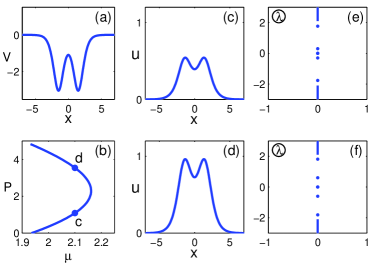
Figure 1: (a) potential (28) in Example 1; (b) power curve of solitons; (c,d) soliton profiles at points marked by the same letters in (b); (e,f) stability spectra of solitons in (c,d).

Example 2. We still consider Eq. (27) but now with a complex PT-symmetric potential

$$V(x) = -3\left[\mbox{sech}^{2}(x+1.5)+\mbox{sech}^{2}(x-1.5)\right]$$ (29)

$$+0.25i\left[\mbox{sech}^{2}(x+1.5)-\mbox{sech}^{2}(x-1.5)\right],\hskip 14.22636pt$$

see Fig. 2(a). This nonconservative system still admits solitary waves (2) for continuous real ranges of $\mu$, but $u(x)$ is complex-valued now. We have numerically obtained a family of these solitons, whose power curve is plotted in Fig. 2(b). Again a saddle-node bifurcation can be seen at $\mu_{0}\approx 2.02$. For solitary waves on the lower and upper branches near this bifurcation point (see Fig. 2(c,d)), their stability spectra lie entirely on the imaginary axis (see Fig. 2(e,f)), indicating that they are all linearly stable. Hence no stability switching occurs at saddle-node bifurcations in this nonconservative system either.

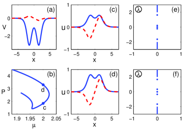
Figure 2: (a) PT potential (29) in Example 2; (b) power curve of solitons; (c,d) soliton profiles at points ‘c,d’ in (b); (e,f) stability spectra of solitons in (c,d). In (a,c,d), solid line is the real part, and dashed line is the imaginary part.

In summary, we have shown that for solitary waves in the generalized NLS equations (1) with real or complex potentials, stability does not switch at saddle-node bifurcations. This disproves a wide-spread belief that such stability switching should always occur in nonlinear partial differential equations. Since the generalized NLS equations (1) arise frequently in nonlinear optics, Bose-Einstein condensates and other physical disciplines, our finding could have broad impact.

References

- (1) J. Guckenheimer and P. Holmes, Nonlinear Oscillations, Dynamical Systems, and Bifurcations of Vector Fields (Springer-Verlag, New York 1990).
- (2) B. Buffoni, A. R. Champneys, and J. F. Toland, J. Dyn. Differ. Equ. 8, 221 (1996).
- (3) T.S. Yang and T.R. Akylas, J. Fluid Mech. 30, 215 (1997).
- (4) M. Chen, Appl. Anal. 75, 213 (2000).
- (5) J. Burke and E. Knobloch, Chaos 17, 037102 (2007).
- (6) G. Herring, P.G. Kevrekidis, R. Carretero-Gonz lez, B.A. Malomed, D.J. Frantzeskakis, and A.R. Bishop, Phys. Lett. 345, 144 (2005).
- (7) T. Kapitula, P. Kevrekidis, and Z. Chen, SIAM J. Appl. Dyn. 5, 598 (2006).
- (8) A. Sacchetti, Phys. Rev. Lett. 103, 194101 (2009).
- (9) T.R. Akylas, G. Hwang and J. Yang, Proc. Roy. Soc. A, doi: 10.1098/rspa.2011.0341 (2011).
- (10) F. Dalfovo, S. Giorgini, L. P. Pitaevskii and S. Stringari, Rev. Mod. Phys. 71, 463 (1999).
- (11) Y. S. Kivshar and G. P. Agrawal, Optical Solitons: From Fibers to Photonic Crystals (Academic Press, San Diego, 2003).
- (12) J. Yang, Nonlinear Waves in Integrable and Nonintegrable Systems (SIAM, Philadelphia, 2010).
- (13) C.M. Bender and S. Boettcher, Phys. Rev. Lett. 80, 5243 (1998).