HPQCD collaboration

Prediction of the bottomonium D-wave spectrum from full lattice QCD

Abstract

We calculate the full spectrum of $D$-wave states in the $\Upsilon$ system in lattice QCD for the first time, using an improved version of NonRelativistic QCD on coarse and fine ‘second generation’ gluon field configurations from the MILC collaboration that include the effect of up, down, strange and charm quarks in the sea. Taking the $2S-1S$ splitting to set the lattice spacing, we determine the ${}^{3}D_{2}-1\overline{S}$ splitting to 2.3%, and find agreement with experiment. Our prediction of the fine structure relative to the ${}^{3}D_{2}$ gives the ${}^{3}D_{3}$ at 10.181(5) GeV and the ${}^{3}D_{1}$ at 10.147(6) GeV. We also discuss the overlap of ${}^{3}D_{1}$ operators with ${}^{3}S_{1}$ states.

Introduction. The spectrum of $b\overline{b}$ states has provided a very important testing ground for strong interaction physics because of the number of radial and orbital excitations that are ‘gold-plated’, i.e. well below the threshold for decay to $B$ mesons. The recent discovery of the $\eta_{b}(1S)$ Aubert et al. (2008) and $h_{b}(1P)$ and $h_{b}(2P)$ mesons Adachi et al. (2011) filled in important gaps in the spin-singlet states. The mass of the $\eta_{b}$ meson had previously been predicted by lattice QCD Gray et al. (2005) and the $h_{b}$ meson masses were widely expected, and found, to be very close to the spin-average of their associated spin-triplet states.

The key missing gold-plated mesons are now the $\Upsilon(1D)$ states. These are very difficult to find experimentally although the ${}^{3}D_{2}$ has been seen in radiative decay from the $\Upsilon(3S)$ Bonvicini et al. (2004). Masses of the $D$-wave states have been predicted in potential model calculations (see, for example Kwong and Rosner (1988); Brambilla et al. (2004)), but it is hard to quantify the errors in these predictions except by using different forms for the potentials.

In lattice QCD the starting point is QCD itself. The difficulties with the $D$-wave states then stem from the signal to noise ratio; the signal falls exponentially in lattice time with the $D$-wave mass but the noise falls with the smaller ground state $S$-wave mass. Very large samples of meson correlators on full QCD gluon field configurations are then needed to obtain a reliable signal. Here we give the first results from lattice QCD that are able to distinguish the fine structure of $D$-wave states.

Lattice Calculation. We use ‘second generation’ gluon field configurations recently generated by the MILC collaboration Bazavov et al. (2010a). These have a gluon action fully improved through $\alpha_{s}a^{2}$ Hart et al. (2009) and include the effect of $u$, $d$, $s$ and $c$ quarks in the sea using the Highly Improved Staggered Quark formalism Follana et al. (2007). The $u$ and $d$ quarks have the same mass, $m_{l}$, so the configurations are denoted as $n_{f}=2+1+1$. We use three ensembles to give two values of the lattice spacing and two values of $m_{l}$. The parameters of the ensembles are given in Table 1; we label them as 3, 4 and 5 from earlier work Dowdall et al. (2011) in which we mapped out the $S$ and $P$-wave bottomonium spectrum and determined the lattice spacing from the $\Upsilon$ $(2S-1S)$ splitting.

We calculate $b$ quark propagators on these configurations using an improved lattice discretisation of NonRelativistic QCD (NRQCD). NRQCD is an expansion in powers of the heavy quark velocity and therefore good for $b$ quarks since $v^{2}/c^{2}\approx 0.1$ inside their bound states. The Hamiltonian includes all terms through $\mathcal{O}(v^{4})$ Dowdall et al. (2011):

$$aH = -\frac{\Delta^{(2)}}{2am_{b}}$$

$$-c_{1}\frac{(\Delta^{(2)})^{2}}{8(am_{b})^{3}}+c_{2}\frac{i}{8(am_{b})^{2}}\left(\bf{\nabla}\cdot\tilde{\bf{E}}\right.-\left.\tilde{\bf{E}}\cdot\bf{\nabla}\right)$$

$$-c_{3}\frac{1}{8(am_{b})^{2}}\bf{\sigma}\cdot\left(\tilde{\bf{\nabla}}\times\tilde{\bf{E}}\right.-\left.\tilde{\bf{E}}\times\tilde{\bf{\nabla}}\right)$$

$$-c_{4}\frac{1}{2am_{b}}\,{\bf{\sigma}}\cdot\tilde{\bf{B}}+c_{5}\frac{\Delta^{(4)}}{24am_{b}}-c_{6}\frac{(\Delta^{(2)})^{2}}{64(am_{b})^{2}}.$$

Here $\nabla$ is the symmetric lattice derivative and $\Delta^{(n)}$ is the lattice discretization of the continuum $\sum_{i}D_{i}^{n}$. $\bf\tilde{E}$ and $\bf\tilde{B}$ are the chromoelectric and chromomagnetic fields. $am_{b}$ is the bare $b$ quark mass, which is tuned by determination on the lattice of the spin-average of ground-state $\Upsilon$ and $\eta_{b}$ meson masses. This was done in Dowdall et al. (2011) to give the values used here, quoted in Table 2.

The $v^{4}$ terms in $\delta H$ have coefficients $c_{i}$ whose values are fixed from matching lattice NRQCD to full QCD, either perturbatively or nonperturbatively. Here we use coefficients for $c_{1}$, $c_{5}$ and $c_{6}$ that include $\mathcal{O}(\alpha_{s})$ corrections, as described in Dowdall et al. (2011). The coefficients $c_{3}$ and $c_{4}$ of the spin-dependent $v^{4}$ terms have been tuned from a study of the fine structure of the $\chi_{b}(1P)$ states. We find $c_{3}=1.0$ with an error of 0.1. $c_{4}$ is significantly larger. Here we use $c_{4}$ = 1.25 on the coarse lattices and 1.10 on the fine lattices. These agree within 0.1 both with the value required to give $P$-wave fine structure in agreement with experiment and with the $\mathcal{O}(\alpha_{s})$ improved result Dowdall et al. (2011).

To make meson correlators for $D$-wave states we use a quark propagator made from either a local or a smeared source which has appropriate derivatives applied to it to generate a $D$-‘wavefunction’. This propagator is then combined with a local propagator and the same derivatives and smearings applied at the sink to create a $2\times 2$ matrix of correlators for each $D$-wave state. The complete set of combinations of spin matrices and derivatives needed is given in Davies et al. (1994). Note that the spin-2 and spin-3 representations split into irreducible representations of the lattice rotational group $\{A_{1},A_{2},E,T_{1},T_{2}\}$, which must be considered independently since their masses can differ by discretisation errors. Very high statistics is required - we have typically 32,000 correlators for every source operator per ensemble, using multiple time sources per configuration. The time sources are binned over for analysis.

Bayesian fitting Lepage et al. (2002) is used to extract the spectrum from the correlators using fit function:

$$G_{\mathrm{meson}}(n_{sc},n_{sk};t)=\sum_{k=1}^{n_{\rm{exp}}}a(n_{sc},k)a^{*}(n_{sk},k)e^{-E_{k}t}.$$ (2)

$E_{k}$ is the energy of the $(k-1)$th radial excitation and $a(n,k)$ label the amplitudes depending on source and sink smearing. We fit all the $D$-wave states together taking the ${}^{3}D_{2}E$ state as the reference state, with a prior of width 0.1 on its ground-state energy. Relative to that we take prior value $0\pm 40$ MeV on the ground-state energy of the other states. We take priors $0.5\pm 0.5$ GeV on radial excitation energies and $0.1\pm 1.0$ on amplitudes. We fit correlators from time $t/a$ = 2 to 12 except for the local-local correlators which we take from $t/a$ = 9 to 12.

Table 1: Details of the MILC gluon field ensembles used in this paper. $a$ is the lattice spacing in fm determined from the $\Upsilon$ $(2S-1S)$ splitting and $L/a$ and $T/a$ give the lattice size. $am_{l},am_{s}$ and $am_{c}$ are the sea quark masses in lattice units. Ensembles 3 and 4 are denoted “coarse” and 5, “fine.”

Set	$a$ (fm)	$am_{l}$	$am_{s}$	$am_{c}$	$L/a\times T/a$
3	0.1219(9)	0.0102	0.0509	0.635	24$\times$64
4	0.1195(10)	0.00507	0.0507	0.628	32$\times$64
5	0.0884(6)	0.0074	0.037	0.440	32$\times$96

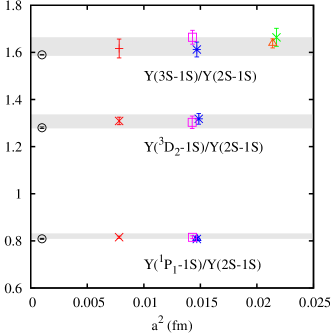
Figure 1: Results for the ratio of the $1^{3}D_{2}-1S$ splitting to the $2S-1S$ splitting in the $\Upsilon$ system plotted against the square of the lattice spacing determined from the $2S-1S$ splitting. Other ratios from Dowdall et al. (2011) are shown for comparison. The grey shaded bands give the physical result obtained from a fit to the data as described in the text, and with the full error of Table 3. The black open circles slightly offset from $a=0$ are from experiment Nakamura et al. (2010).

Table 2: Fitted $D$-wave energies on each ensemble. Errors are from statistics/fitting only. $c_{3}=1.0$ on all ensembles, $c_{4}=1.25$ on sets 3 and 4 and 1.10 on set 5. $a\Delta(x)=aE(x)-aE(^{3}\overline{D})$. $R_{X}$ and $\Delta_{X}$ are defined in the text. The $A_{2}$ irrep. on set 5 is fit separately and not included in the splittings.

	Set 3	Set 4	Set 5
	$am_{b}=2.66$	$am_{b}=2.62$	$am_{b}=1.91$
$aE(1^{1}D_{2E})$	0.705(10)	0.694(12)	0.594(5)
$aE(1^{1}D_{2T_{2}})$	0.711(8)	0.693(10)	0.589(3)
$aE(1^{3}D_{1T_{1}})$	0.695(7)	0.680(10)	0.575(8)
$aE(1^{3}D_{2E})$	0.698(10)	0.692(10)	0.588(4)
$aE(1^{3}D_{2T_{2}})$	0.702(8)	0.691(10)	0.589(4)
$aE(1^{3}D_{3A_{2}})$	0.707(10)	0.704(10)	0.597(4)
$aE(1^{3}D_{3T_{1}})$	0.715(7)	0.705(8)	0.596(4)
$aE(1^{3}D_{3T_{2}})$	0.714(7)	0.696(9)	0.594(3)
$a\Delta(1^{1}D_{2})$	0.0029(31)	0.0004(37)	0.0027(27)
$a\Delta(1^{3}D_{1})$	-0.0104(34)	-0.0137(44)	-0.0137(62)
$a\Delta(1^{3}D_{2})$	-0.0047(23)	-0.0021(21)	0.0001(20)
$a\Delta(1^{3}D_{3})$	0.0078(22)	0.0074(27)	0.0069(20)
$R_{D}$	1.318(23)	1.303(26)	1.309(16)
$a\Delta_{\bf L\cdot S}$	0.0038(11)	0.0040(13)	0.0037(13)
$a\Delta_{S_{ij}}$	-0.0005(9)	0.0009(9)	0.0016(15)
$R_{\bf L\cdot S}$	0.44(13)	0.49(17)	0.60(21)
$R_{S_{ij}}$	-0.26(52)	0.53(50)	1.1(1.0)

Results. The results from our fits for each $D$-wave lattice representation on each ensemble are given in Table 2. We use $n_{\rm{exp}}=3$ on sets 3 and 4 and $n_{\rm{exp}}=4$ on set 5 since these have the highest posterior probability Lepage et al. (2002); values and errors have stabilised at this point and $\chi^{2}/{\rm{dof}}<1$. We also give the ratio $R_{D}=(1^{3}D_{2}-1\overline{S})/(2^{3}S_{1}-1^{3}S_{1})$ where $1\overline{S}$ is the spin-average of $\Upsilon$ and $\eta_{b}$ energies from Dowdall et al. (2011) and $1^{3}D_{2}$ is the dimension-weighted average of the lattice ${}^{3}D_{2E}$ and ${}^{3}D_{2T_{2}}$ results.

$R_{D}$ is plotted along with similarly defined $R_{S}$ and $R_{P}$ from Dowdall et al. (2011) in Figure 1. To obtain a physical result for $R_{D}$ we fit to the same form used in Dowdall et al. (2011) for $R_{S}$ and $R_{P}$, allowing for lattice spacing and sea quark mass dependence:

$$R = R_{\mathrm{phys}}[1+2b_{l}\delta x_{l}(1+c_{l}(a\Lambda)^{2})$$

$$+ \sum_{j=1,2}c_{j}(a\Lambda)^{2j}(1+c_{jb}\delta x_{m}+c_{jbb}(\delta x_{m})^{2})].$$

Here $\delta x_{l}$ is $(am_{l}/am_{s})-(m_{l}/m_{s})_{\mathrm{phys}}$ for each ensemble. $(m_{l}/m_{s})_{\mathrm{phys}}$ is taken from lattice QCD as 27.2(3) Bazavov et al. (2010b). $\delta x_{m}=(am_{b}-2.65)/1.5$ allows for $am_{b}$ effects from NRQCD in the discretisation errors over our range of $a$ values. $\Lambda$, taken as 500 MeV, sets the scale for physical $a$-dependence. Fit priors are as in Dowdall et al. (2011): 1.0(0.5) on $R_{\mathrm{phys}}$; 0.0(0.3) on $a^{2}$ terms; 0.0(1.0) on higher order in $a$; 0.0(0.015) on $b_{l}$. The physical result we obtain for $R_{D}$ is 1.307(30), after adding an additional NRQCD systematic error for missing $v^{6}$ terms Dowdall et al. (2011). This is to be compared to the experimental value of 1.280(3). A complete error budget for $R_{D}$ is given in Table 3.

Table 3: Complete error budget for $R_{D}$ in %. Finite volume and $m_{b}$ tuning errors are negligible.

	$R_{D}$
stats/fitting	1.4
$a$-dependence	1.4
$m_{l}$-dependence	0.5
NRQCD $am_{b}$-dependence	0.1
NRQCD systematics	1.0
electromagnetism/$\eta_{b}$ annihilation	0.2
Total	2.3%

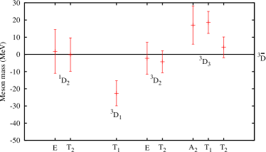
Figure 2: Results for the separate irreducible representations of the lattice rotation group making up each continuum $D$-wave state on coarse set 4.

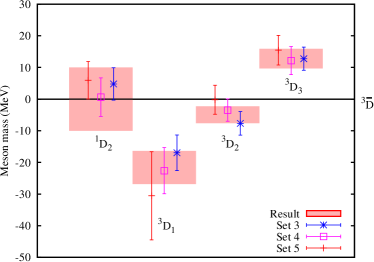
Figure 3: $D$-wave masses plotted relative to the ${}^{3}D$ spin-average for all sets using the $2S-1S$ splitting to set the scale. The red shaded bands show our final results using ratios of combinations of splittings to those of $P$-wave states as described in the text.

Figure 4: Ratios $R_{S_{ij}}$ and $R_{\bf L\cdot S}$ (multiplied by -5 for clarity) plotted against the square of the lattice spacing. The grey bands give our physical results.

In Figure 2 we plot the masses of all the lattice representations relative to the spin average of all $1^{3}D$ states for coarse set 4, using the $2S-1S$ splitting to set the scale (Table 1). We see that the lattice representations for each spin agree well with each other within our sizeable statistical errors. The hyperfine splitting, between the ${}^{1}D_{2}$ and the spin average of ${}^{3}D$ states is expected to be very small, following results for $P$-wave states. We find it to be zero to within 10 MeV.

Figure 3 shows the results from all three sets, using a dimension-weighted average of results, including the correlations from the fit, for the different lattice representations for the ${}^{3}D_{3}$ and ${}^{(1,3)}D_{2}$. Results are consistent between the fine and coarse sets and between different sea light quark masses for the two coarse sets.

To arrive at a final result for $D$-wave fine structure we study combinations of ${}^{3}D$ spin-splittings that are sensitive either to an $\bf{L}\cdot\bf{S}$ or to a tensor $S_{ij}$ interaction ($\bf{S}\cdot\bf{S}$ takes the same value for all ${}^{3}D$ states). Writing

$$M_{J}=\overline{M}({}^{3}D)+\Delta^{D}_{L\cdot S}\langle\bm{L}\cdot\bm{S}\rangle+\Delta^{D}_{S_{ij}}\langle S_{ij}\rangle$$ (4)

gives

$$\Delta^{D}_{L\cdot S} = (14M_{3}-5M_{2}-9M_{1})/60$$

$$\Delta^{D}_{S_{ij}} = -7(2M_{3}-5M_{2}+3M_{1})/120.$$ (5)

Table 2 gives our results for these splittings. In Figure 4 we plot ratios to the equivalent ${}^{3}P$ splitting combinations: $R_{X}=\Delta^{D}_{X}/\Delta^{P}_{X}$ with $\Delta^{P}_{L\cdot S}=(5M_{2}-3M_{1}-2M_{0})/12$ and $\Delta^{P}_{S_{ij}}=-5(M_{2}-3M_{1}+2M_{0})/72$. Values for $\Delta^{P}$ for these ensembles are given in Dowdall et al. (2011) (without factors of 1/12 and -5/72). The experimental values are $\Delta^{P}_{L\cdot S}$ = 13.65(27) MeV and $\Delta^{P}_{S_{ij}}$ = 3.29(9) MeV Nakamura et al. (2010). The advantage of using these combinations is that they depend purely on one of the spin-dependent coefficients of the NRQCD action. On set 5 we did not use exactly the same values for $c_{3}$ and $c_{4}$ in our study of $P$ and $D$ waves. However we can correct for this in Figure 4 since $\Delta_{S_{ij}}\propto c_{4}^{2}$ and $\Delta_{L\cdot S}\propto c_{3}$. Once this slight adjustment is done the dependence on $c_{3,4}$ cancels between $P$ and $D$ states and so errors from the uncertainty in these coefficients are much reduced.

We fit the fine-structure $R$ values to the same form used earlier in eq. Prediction of the bottomonium D-wave spectrum from full lattice QCD to extract physical results:

$$R_{L\cdot S}=0.49(11);\quad R_{S_{ij}}=0.26(35).$$ (6)

We have included an additional systematic error of 10% to allow for missing $v^{6}$ terms from our NRQCD action but the lattice statistical error dominates. We then combine the $R$ values with experimental results from $1P$ levels to give the following ${}^{3}D$ splittings:

$${}^{3}D_{3}-{}^{3}D_{1} = 34(8)\mathrm{MeV}$$

$${}^{3}D_{3}-{}^{3}D_{2} = 18(5)\mathrm{MeV}$$

$${}^{3}D_{2}-{}^{3}D_{1} = 17(6)\mathrm{MeV}.$$ (7)

Our fine structure splittings are somewhat larger than typical results from potential models Kwong and Rosner (1988); Brambilla et al. (2004), where the ${}^{3}D_{3}-{}^{3}D_{1}$ splitting lies in the range 10-20 MeV. This can be traced to a larger value for $R_{L\cdot S}$ than is obtained, for example, in Kwong and Rosner (1988), based on specific forms for the spin-dependent potentials.

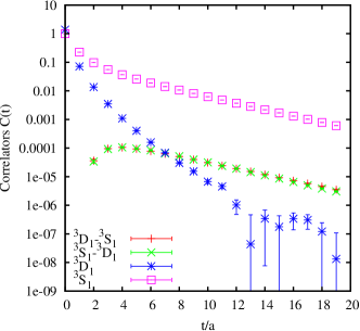
Figure 5: Correlators made from different combinations of local ${}^{3}S_{1}$ and ${}^{3}D_{1}$ operators at source and sink, plotted with a logarithmic $y$ axis as a function of lattice time, $t$. Results are from set 3.

One issue that we have neglected above is that the ${}^{3}D_{1}$ state has $J^{PC}=1^{--}$ in common with ${}^{3}S_{1}$ states. On the lattice, in principle, any operator with $1^{--}$ quantum numbers will be able to create all $1^{--}$ states. In practice the amplitude for ${}^{3}S_{1}$ states to be created by the operators that we use for the ${}^{3}D_{1}$ is very small and vice versa. We illustrate that in Fig. 5 where we show correlators from set 3 that use a local ${}^{3}S_{1}$ or ${}^{3}D_{1}$ operator at source and sink compared to the cross-correlator that has a local ${}^{3}S_{1}$ operator at the source and ${}^{3}D_{1}$ at sink or vice versa. The cross-correlator is much smaller in magnitude than either of the diagonal correlators at small $t$ values. The exponential fall-off (as seen in the slope of the log plot) of the cross-correlator matches that of the ${}^{3}S_{1}$ correlator at large times, where the ${}^{3}D_{1}$ correlator fall-off is dominated by that of the heavier ${}^{3}D_{1}$ state. If we fit the complete set of ${}^{3}S_{1}$ and ${}^{3}D_{1}$ correlators together, including the local cross-correlators of Fig. 5, we obtain results in agreement with our separate fits for ${}^{3}S_{1}$ (in Dowdall et al. (2011)) and ${}^{3}D_{1}$ masses. We also find, for example, that the amplitude $a({}^{3}D_{1,local},\Upsilon)$ from eq. 2 is 0.0052(1) times that of $a({}^{3}S_{1,local},\Upsilon)$.

Conclusions. We give the first full lattice QCD results for the $D$-wave states of bottomonium including the fine structure. We obtain a mass of 10.179(17) GeV for the $1^{3}D_{2}$ to be compared with 10.1637(14) GeV from experiment Nakamura et al. (2010). Using the experimental result for the $1^{3}D_{2}$ mass we predict masses of 10.181(5) GeV for the $1^{3}D_{3}$, 10.147(6) GeV for the $1^{3}D_{1}$ and 10.169(10) for the ${}^{1}D_{2}$.

Acknowledgements. We are grateful to MILC for the use of their gauge configurations and to Peter Lepage for comments. We used the Darwin Supercomputer under the DiRAC facility jointly funded by STFC, BIS and the Universities of Cambridge and Glasgow. This work was funded by STFC and the EU Erasmus programme.

References

- Aubert et al. (2008) B. Aubert et al. (BABAR), Phys. Rev. Lett. 101, 071801 (2008), eprint 0807.1086.
- Adachi et al. (2011) I. Adachi et al. (Belle) (2011), eprint 1103.3419.
- Gray et al. (2005) A. Gray et al. (HPQCD), Phys.Rev. D72, 094507 (2005), eprint hep-lat/0507013.
- Bonvicini et al. (2004) G. Bonvicini et al. (CLEO), Phys. Rev. D70, 032001 (2004), eprint hep-ex/0404021.
- Kwong and Rosner (1988) W. Kwong and J. L. Rosner, Phys. Rev. D38, 279 (1988).
- Brambilla et al. (2004) N. Brambilla et al. (Quarkonium Working Group) (2004), eprint hep-ph/0412158.
- Bazavov et al. (2010a) A. Bazavov et al. (MILC), Phys.Rev. D82, 074501 (2010a), eprint 1004.0342.
- Hart et al. (2009) A. Hart, G. M. von Hippel, and R. R. Horgan (HPQCD), Phys. Rev. D79, 074008 (2009), eprint 0812.0503.
- Follana et al. (2007) E. Follana et al. (HPQCD), Phys.Rev. D75, 054502 (2007), eprint hep-lat/0610092.
- Dowdall et al. (2011) R. J. Dowdall et al. (HPQCD) (2011), eprint 1110.6887.
- Davies et al. (1994) C. T. H. Davies et al., Phys. Rev. D50, 6963 (1994), eprint hep-lat/9406017.
- Lepage et al. (2002) G. P. Lepage et al., Nucl. Phys. Proc. Suppl. 106, 12 (2002), eprint hep-lat/0110175.
- Nakamura et al. (2010) K. Nakamura et al. (Particle Data Group), J. Phys. G37, 075021 (2010).
- Bazavov et al. (2010b) A. Bazavov et al., Rev. Mod. Phys. 82, 1349 (2010b), eprint 0903.3598.