Magnetic Response in the Underdoped Cuprates

Abstract

We examine the dynamical magnetic response of the underdoped cuprates by employing a phenomenological theory of a doped resonant valence bond state where the Fermi surface is truncated into four pockets. This theory predicts a resonant spin response which with increasing energy (0 to 100meV) appears as an hourglass. The very low energy spin response is found at $(\pi,\pi\pm\delta)$ and $(\pi\pm\delta,\pi)$ and is determined by scattering from the pockets’ frontside to the tips of opposite pockets where a van Hove singularity resides. At energies beyond 100 meV, strong scattering is seen from $(\pi,0)$ to $(\pi,\pi)$. This theory thus provides a semi-quantitative description of the spin response seen in both INS and RIXS experiments at all relevant energy scales.

Introduction: Neutron scattering studies of the magnetic properties of underdoped cuprate superconductors have revealed an unusual ‘hourglass’ pattern in the spin excitation spectrum that persists into the normal state review1 . This spectrum which is centered on $(\pi,\pi)$, can be divided into three energy regions. At low energies the weight is shifted to nearby incommensurate wavevectors, peaking along the crystal axes. With increasing energy the weight is more uniformly distributed around $(\pi,\pi)$ and contracts to form a resonance centered on $(\pi,\pi)$. At still higher energies a uniform ring appears evolving away from $(\pi,\pi)$. Recent RIXS experiments rixs have explored this high energy region further.

A phenomenological theory for the underdoped pseudogap phase by Yang, Rice and Zhang (YRZ) yrz has had considerable success in reproducing many electronic properties yrz_review . In this letter we examine the spin spectrum within this theory and show that key features of the experiments at all three energies are reproduced. We begin with a derivation of the YRZ ansatz starting from a t- J model rather than from the overdoped Fermi liquid in the original paper, following a recent suggestion by P. A. Lee pl_private which in turn is based on a small modification of Ref. ng . An RPA form is used for the spin response similar to that employed by Brinckman and Lee in their study of the spin resonance in the superconducting state of overdoped cuprates. The itinerant description in our approach differs from the often used scenario of strong and slow stripe fluctuations which would show up as incommensurate quasi-elastic peaks in the magnetic response stripes . We compare our results with data sets gathered using both x-rays and neutrons.

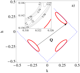
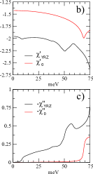
Figure 1: a) The Fermi surface for hole doping, $x=0.12$. Hole pockets are marked in red (solid) while the lines of Luttinger zeros are blue (dashed). Also marked is a nesting vector ${\bf Q}=(0.5,0.375)$ (in reciprocal lattice units), connecting the tip of a pocket to the frontside of another pocket. Inset: A plot demonstrating that at the tip of the pocket there is a saddlepoint in the superconducting quasi-particle dispersion and hence a van Hove singularity. Contours are labelled in meV. The parameters used here are $t(x)=70$meV, $t^{\prime}(x)=-0.18t(x)$, $t^{\prime\prime}(x)=0.12t(x)$, $\Delta_{0}=0.34t(x)$ and $\Delta_{SC}=0.05t(x)$. b) The real parts of $\chi_{YRZ}({\bf Q},\omega)$ and $\chi_{0}({\bf Q},\omega)$ vs. $\omega$. c) The imaginary parts.

YRZ Spin Response: The YRZ ansatz, as originally conceived, was an ansatz for the single particle Green’s function (GF) of the underdoped cuprates. The Fermi surface associated with it is truncated and composed of four nodal pockets (see Fig. 1). The area of the pockets is proportional to the level of doping, x. This GF is also characterized by lines of Luttinger zeros which coincide with the magnetic Brillouin zone (BZ) or Umklapp surface honer (see Fig. 1). The ansatz was inspired by an analysis of a system of weakly coupled Hubbard ladders where a similar phenomenology was found to hold krt .

To extend the YRZ ansatz from the single particle GF to the spin response, we first elucidate the connection between YRZ and the slave boson (SB) treatment of the t-J Hamiltonian. SBs provide a natural RPA-like form to the spin response and we intend to adapt this to the assumptions of YRZ. For this purpose we then write the $t-J$ Hamiltonian as

$$H = -\sum_{ij\sigma}t^{nn}_{ij}c^{\dagger}_{i\sigma}c_{j\sigma}-\sum_{ij\sigma}t^{nnn}_{ij}c^{\dagger}_{i\sigma}c_{j\sigma}+\frac{1}{2}\sum_{ij}J_{H}S_{i}\cdot S_{j}$$ (1)

$$\equiv H_{t}^{nn}+H_{t}^{nnn}+H_{J_{H}}$$ (3)

The Hamiltonian is divided into terms involving nearest neighbour (NN) hopping, $H_{t}^{nn}$, terms involving next nearest neighbour (NNN) hopping (and beyond), $H_{t}^{nnn}$, and a spin-spin interaction, $H_{J_{H}}$. We choose this separation because of the focus the YRZ ansatz places upon the Luttinger zeros found at the magnetic BZ. The nearest neighbour dispersion, $\xi_{0}(k)=-2t(x)(\cos k_{x}+\cos k_{y})$ (for the definition of t(x) see yrz ; supp_mat ) vanishes on this line while that of the NNN hopping does not. (We show in the supplementary material supp_mat that one can derive a YRZ-like propagator while treating NN and NNN hopping on the same footing.) We now subject $H_{t}^{nn}+H_{J_{H}}$ to the standard slave boson mean field treatment (leaving $H_{t}^{nnn}$ to later). We thus factor the fermions, $c^{\dagger}_{i\sigma}$, into spinons, $f^{\dagger}_{i\sigma}$ and holons, $b_{i}$ via $c^{\dagger}_{i\sigma}=f^{\dagger}_{i\sigma}b_{i},$ where the spinons and holons are subject to the constraint $\sum_{\sigma}f^{\dagger}_{i\sigma}f_{i\sigma}+b^{\dagger}_{i}b_{i}=1.$ At this level the spinon Green’s function can be shown to be bl

$$G^{f}_{\sigma}(\omega,{\bf k})=\frac{1}{\omega-\xi_{0}({\bf k})-\Sigma_{R}(\omega,{\bf k})},$$ (4)

where $\Sigma_{R}=|\Delta_{R}({\bf k})|^{2}/(\omega+\xi_{0}({\bf k}))$ and $\Delta_{R}({\bf k})=\Delta_{0}(x)(\cos k_{x}-\cos k_{y})$. Here $t(x)$ and $\Delta_{0}(x)$ are doping dependent parameters. The single particle Green’s function, $G^{c}_{\sigma}$, is given directly in terms of the spinon Green’s function because we assume the bosons are nearly condensed and so replace the boson propagator $\langle b_{i}^{\dagger}(\tau)b_{j}(0)\rangle$ by $g_{t}(x)$: $G^{c}_{\sigma}(\omega,{\bf k})=g_{t}(x)G^{f}_{\sigma}(\omega,{\bf k})$ (in slave boson mean field $g_{t}(x)=x$ bl ; in the Gutzwiller approximation $g_{t}(x)=2x/(1+x)$ yrz ). This is close to the YRZ form but differs in that the full dispersion in the denominator is replaced by the dispersion due to NN hopping.

To bridge the gap between the SBMFT and YRZ, we then turn to the so far neglected NNN hopping, $H_{t}^{nnn}$. Treating this term in mean field theory (MFT) moves the Luttinger zeros off the magnetic Brillouin zone and so we instead use an RPA like approximation (see Fig. 2) leading to

$$G^{f}_{\sigma}(\omega,{\bf k}) =\frac{1}{\omega-\xi_{0}({\bf k})-\xi^{\prime}({\bf k})-\Sigma_{R}(\omega,{\bf k})}.$$ (5)

Here $\xi^{\prime}(k)=-4t^{\prime}(x)\cos k_{x}\cos k_{y}-2t^{\prime\prime}(x)(\cos 2k_{x}+\cos 2k_{y})$ is the dispersion due to the NNN terms. The spinon propagator in this form now immediately gives the YRZ ansatz.

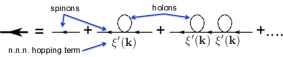
Figure 2: RPA form of the YRZ spinon propagator in terms of SB propagators.

An important consequence of the non-MFT treatment of the $H^{nnn}_{t}$ is that spinons and holons are bound together. This binding distinguishes the YRZ ansatz from the standard mean field SB approximation which leads to an expanded Hilbert space with independent spinons and holons. A second consequence is the absence of an anomalous spinon propagator (or at least the coherent part thereof), consistent with an underlying RVB assumption that spin correlations are short- not long-ranged in the YRZ ansatz.

This form (Eqn. 10) applies in the normal phase and can be generalized to the d-wave superconducting state, e.g. see yrz_review . Note that YRZ gives a two-gap description of the pseudogap phase with a separate RVB ($\Delta_{0}$) and pairing $\Delta_{SC}$ gaps.

We now turn to the YRZ spin response. In slave bosons, neglecting the effects of NNN hopping, the spin response naturally takes on an RPA-like form bl :

$$S(\omega,{\bf k})=-\frac{3}{\pi}\mathrm{Im}\frac{\chi_{0}(\omega,{\bf k})}{1-J({\bf k})\chi_{0}(\omega,{\bf k})}.$$ (6)

Here $\chi_{0}(\omega,{\bf k})$ is the bare particle-hole bubble for the spinons (including anomalous contributions) and $J({\bf{k}})=J(\cos k_{x}+\cos k_{y})$.

How now does our non-mean field treatment of $H^{nnn}_{t}$ alter this? Its effect is two-fold. Firstly we no longer include a contribution to $\chi_{0}$ from the anomalous spinon Green’s functions. And to determine how $t^{nnn}$ dresses the normal spinon Green’s functions, we employ the same approximation that led to the YRZ ansatz. Namely we only allow diagrams involving vertices where the boson lines of the vertex are tied together. Under such a restriction, $t^{nnn}$ only dresses the individual spinon propagators making up the particle-hole bubble entering $\chi_{0}$. In this fashion the YRZ spin ansatz takes the form

$$S_{YRZ}(\omega,{\bf k})=-\frac{3}{\pi}\mathrm{Im}\frac{\chi_{YRZ}(\omega,{\bf k})}{1-J({\bf k})\chi_{YRZ}(\omega,{\bf k})},$$ (7)

where $\chi_{YRZ}$ is simply a particle-hole bubble made up of YRZ quasi-particles.

In computing the spin response we treat $J$ as a fitting parameter for each doping (and different from $J_{H}$). We do not expect the underlying mean field treatment to accurately treat the renormalization of $J$ which is inevitably doping dependent. In particular in the presence of strong scattering connecting the magnetic Brillouin zone boundaries, we expect $J$ to be strongly modified. This is not merely a feature of the YRZ theory but is generic to slave boson flavoured theories. In Ref. bl , $J$ had to be sharply reduced in order to produce an AF ordering transition at approximately the correct doping.

Results: We begin with the lower energy ($\omega<100$meV) spin response in the underdoped cuprates which has a universal hour glass shape review1 ; lsco8.5 ; lsco16a ; lsco16b with strong incommensurate response at low energies (i.e. $\omega\approx 2\Delta_{SC}$) concentrated at four points, $(\pi,\pi\pm\delta)$ and $(\pi\pm\delta,\pi)$. As energy is initially increased this response evolves inwards towards $(\pi,\pi)$ and simultaneously becomes more isotropic in its distribution about ($\pi,\pi$). Whether this inward dispersion reaches $(\pi,\pi)$ is a function of the particular cuprate being examined. As the energy is further increased this inward evolution is reversed and the response moves outwards from ($\pi,\pi$). With this outward dispersion, the response is more isotropically distributed about $(\pi,\pi)$.

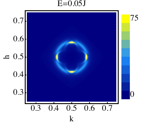
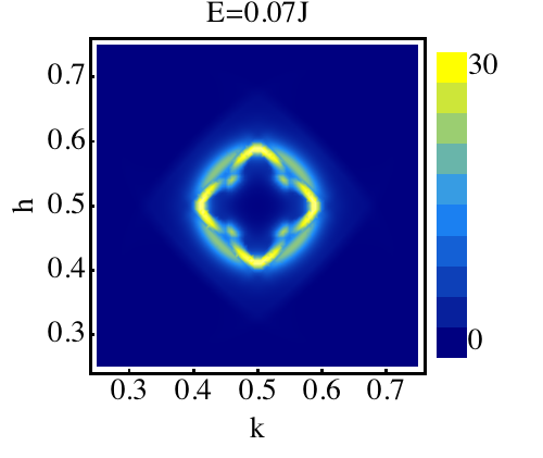
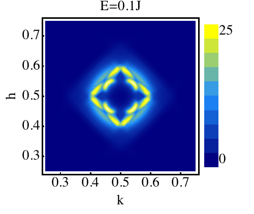
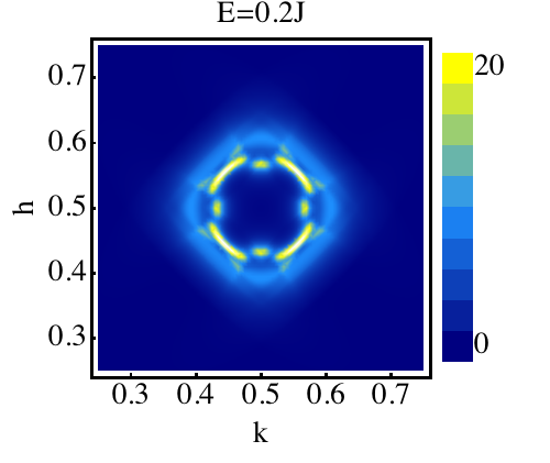
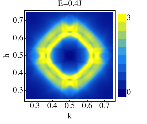
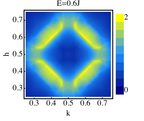
Figure 3: Constant energy slices of the spin response for $x=0.12$ in the SC phase – the parameters used are the same as listed in Fig. 1, with $J=0.14$meV for our theory.

We see these general features in the constant energy scans of the q-dependent spin response presented in Fig. 3 for the superconducting case. In this figure we have chosen parameters appropriate for the description of underdoped $\rm La_{2-x}Sr_{x}CuO_{4}$. We see at very low energies ($0.05J$) the primary response is at $(\pi,\pi\pm\delta)$ and $(\pi\pm\delta,\pi)$ with $\delta=0.16\pi$. As the energy is increased there is a slight inward dispersion ($\delta$ decreases slightly) and the spin response is found circularly distributed about $(\pi,\pi)$. This dispersion reverses at $\omega\sim 0.2J$ and begins to move outwards. In this energy range the greatest response is found about $(\pi\pm\delta^{\prime},\pi\pm\delta^{\prime})$.

The response found at $(\pi,\pi\pm\delta)$ and $(\pi\pm\delta,\pi)$ at $0.05J$meV can be directly ascribed to transitions between the fronts of the pockets and the tips of opposite pockets (see the vector $Q$ in Fig. 1). In general the presence of the pockets in the YRZ theory allows for low energy scattering in a larger portion of the Brillouin zone than in theories where the spinon Fermi surface consists of four points coinciding with nodes of the SC order parameter (see Figs. 1b and 1c for a comparison of $\chi_{YRZ}$ and $\chi_{0}$; $\chi_{0}$ is the bare particle-hole bubble for the standard slave boson description of the spin response bl ). Moreover in the presence of a SC gap, the tips of the pockets see a saddle point in dispersion with a corresponding van Hove singularity thus further enhancing the low energy scattering.

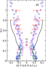
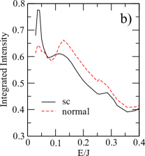
Figure 4: a) Hourglass dispersion of the resonance near $\pi,\pi$. The thick black line is the position of the maximum intensity peak after integrating the numerical data over a strip of width $2\pi/25$ along the parallel direction, averaged over sections of length $2\pi/33$. Experimental data points (appropriately rescaled) are taken from review ; review1 : ‘up’ triangles, La_1.90Sr_0.10CuO₄ lsco8.5 ; circles, La_1.875Ba_0.125CuO₄ jtrannature ; ‘down’ triangles, La_1.84Sr_0.16CuO₄ lsco16b ; squares, YBa₂Cu₃O_6.5 stock and diamonds, YBa₂Cu₃O_6.6 hayden. b) k-integrated spin response with and without a superconducting gap.

With increasing energy, the $\bf k$-points with maximal intensity move inward towards $(\pi,\pi)$, albeit in an uneven fashion (there is a sudden movement inward at $0.125J$) while at the same time becoming more isotropically distributed about $(\pi,\pi)$. This behavior is shared not only by underdoped $\rm La_{2-x}Sr_{x}CuO_{4}$ lsco8.5 but also its optimally doped counterpart lsco16a ; lsco16b . It is also seen in stripe stabilized $\rm La_{2-x}Ba_{x}CuO_{4}$ jtrannature and $\rm YBCO$ review ; review1 . At an energy between $0.4J$ and $0.5J$, the point of maximal intensity begins to drift outward from $(\pi,\pi)$, again a universal feature of the magnetic response in the cuprates. We explicitly plot in Fig. 4a the evolution of the k-point of maximal intensity as a function of energy, comparing its evolution with a number of cuprates.

In the normal state, low energy spectral weight is found not just in directions parallel to the crystal axes but in the nodal directions as well (see Fig. 5). While parallel scattering still dominates at low energies, the response is less concentrated in such areas and weight does appear along the nodal directions (at least in the LSCO family) lsco8.5 ; lsco16a .

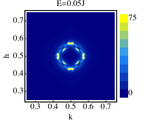
Figure 5: $x=0.12$ and $\omega=7$meV constant energy slices for the SC phase (left) and the normal phase (right).

Underlying our calculations of the magnetic response is the assumption that itinerant quasi-particles (even if heavily dressed) can explain this response in the cuprates. While there is evidence that at least part of the spin response must be ascribed to localized spins jtrannature ; bscco , there is also evidence that impurities introduce local spins, e.g. Zn doped into YBCO ZnYBCO and earlier studies. The full cuprate magnetic response requires a mixture of the two. However one experimental feature of the spin response that points to itinerant quasi-particles is the depression of the k-integrated spin response at $\omega<2\Delta_{SC}$ upon decreasing $T<T_{c}$. This behavior is seen in both the LSCO lsco8.5 ; lsco16a ; lsco16b and $\rm YBCO$ families and we see it as well in our calculations (Fig. 4b). We also see in Fig. 4b that our calculated integrated intensity has a two peak structure, with one peak at energies close to $0.05J$ and one at energies at $\approx 0.12J$. This doubling of peaks is seen in near optimally doped LSCO lsco16a ; lsco16b . In underdoped LSCO at least the lower energy peak has been observed lsco8.5 .

Turning to high energies, $\omega>100$meV, we find the YRZ spin response is also able to explain key features in the spin response recently measured by RIXS experiments. In Fig. 6 we plot the spin response for energies $100{\rm meV}<\omega<300{\rm meV}$ for two cuts in the Brillouin zone. We see two features emanating from $(0,0)$. One disperses towards $(\pi,0)$ as energy is increased (corresponding well with the reported paramagnon-like excitation in the RIXS data of rixs on a variety of cuprates). The other, with a considerably greater spin velocity, evolves towards $(\pi,\pi)$. This dispersing paramagnon excitation naturally appears from a two-band factorization of YRZ where the propagator can be written in the form yrz_review

$$G^{c}_{\sigma}(\omega,{\bf k})=\frac{z_{+}({\bf k})}{\omega-\omega_{+}({\bf k})}+\frac{z_{-}({\bf k})}{\omega-\omega_{-}({\bf k})}.$$ (8)

The paramagnon results from a particle-hole excitation from the lower band, $\omega_{-}({\bf k})$, to the upper band, $\omega_{+}({\bf k})$.

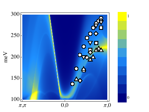
Figure 6: The spin response for energies from 100meV to 300meV, for cuts from $(\pi,\pi)$ to $(0,0)$ to $(\pi,0)$ in the Brillouin zone (same choice of parameters as previously). Also plotted are data points from rixs : circles, Nd_1.2Ba_1.8Cu₃O₆; squares, YBa₂Cu₃O₇; diamonds, Nd_1.2Ba_1.8Cu₃O₇; ‘up’ triangles, YBa₂Cu₄O₈; ‘down’ triangles, YBa₂Cu₃O_6.6.

In conclusion we have shown that calculations of the magnetic response based upon itinerant YRZ quasi-particles reproduces key features reported in experiments on the spin response of the underdoped cuprates at both low and high energies in a satisfactory way.

The authors acknowledge support from the CES, an ERFC funded by the DOE’s OBES. We also thank J. Tranquada, J. Hill, and M. Dean for useful conversations.

Appendix A Supplementary material

In this appendix we give an alternate derivation of YRZ from SBMFT that does not depend on treating the nearest neighbour hopping term in the Hamiltonian, $H^{nn}_{t}$, on a different footing than $H^{nnn}_{t}$.

Here we instead divide the full Hamiltonian into its Heisenberg piece, $H_{J_{H}}$, and its hopping terms, $H_{t}^{nn}+H^{nnn}_{t}$. We first focus on treating $H_{J_{H}}$ in SBMFT. Using standard SBMFT, we find that the spinon propagator is now given by

$$G^{f}_{\sigma}(\omega,{\bf k})=\frac{1}{\omega-\tilde{\xi}_{0}({\bf k})-\frac{|\Delta_{R}({\bf k})|^{2}}{\omega+\tilde{\xi}_{0}({\bf k})}},$$ (9)

where

$$\tilde{\xi}_{0}({\bf k})=-2\tilde{t}(x)(\cos k_{x}+\cos k_{y}).$$

$\tilde{\xi}_{0}$ differs from $\xi_{0}$ in that $\tilde{t}(x)=3/8g_{s}(x)J_{H}\chi$ instead of $t(x)=g_{t}(x)t_{0}+3/8g_{s}(x)J_{H}\chi$ where $t_{0}$ is the bare nearest neighbour hopping strength, $J_{H}$ is the bare Heisenberg coupling, $g_{s}(x)$ is the amount $J_{H}$ is renormalized in the Gutzwiller projection, and $\chi=0.338$. We note that at zero doping ($x=0$), this propagator coincides with the SB propagator in Eqn. (2).

To treat the remaining hopping terms, $H_{t}^{nn}+H^{nnn}_{t}$, we now proceed as we did with $H^{nnn}_{t}$ alone in the main text. Using an RPA approximation, we find for this version of the YRZ propagator

$$G^{f}_{\sigma}(\omega,{\bf k}) = \sum_{n=0}^{\infty}(\tilde{\xi}^{\prime}({\bf k}))^{n}G^{f}_{\sigma}|_{\xi^{\prime}({\bf k})=0}(\omega,{\bf k}))^{n+1}$$ (10)

$$= \frac{1}{\omega-\tilde{\xi}_{0}({\bf k})-\tilde{\xi}^{\prime}({\bf k})-\frac{|\Delta_{R}({\bf k})|^{2}}{\omega+\tilde{\xi}_{0}({\bf k})}},$$ (11)

where now

$$\tilde{\xi}^{\prime}({\bf k})=-2g_{t}(x)t_{0}+\xi^{\prime}({\bf k}).$$

Most importantly, this YRZ propagator retains a line of Luttinger zeros along the magnetic BZ or Umklapp surface.

References

- (1) For a recent review see M. Fujita et al., J. Phys. Soc. Jpn. (in press); arXiv:1108.4431.
- (2) K.-Y. Yang, T. M. Rice, and F.-C. Zhang, Phys. Rev. B 73, 174501 (2006).
- (3) T. M. Rice, K.-Y. Yang, and F.-C. Zhang, arXiv 1109.0632.
- (4) Private communication from P. A. Lee.
- (5) T.K. Ng, Phys. Rev. B 71, 172509 (2005).
- (6) C. Honerkamp et al., Phys. Rev. B 63, 035109 (2001).
- (7) G.S. Uhrig et al., J. Phys. Soc. Jpn. 74 Supplement 86 (2005).
- (8) R. M. Konik, T. M. Rice, and A. Tsvelik, Phys. Rev. Lett. 96, 086407 (2006).
- (9) J. Brinckmann and P. Lee, Physical Review B 65, 014502 (2001).
- (10) See supplementary material.
- (11) O. J. Lipscombe, B. Vignolle, T. G. Perring, C. D. Frost, and S. M. Hayden, Phys. Rev. Lett. 102, 167002 (2009).
- (12) N. B. Christensen et al., Phys. Rev. Lett. 93, 147002 (2004).
- (13) B. Vignolle, et al., Nature Physics 3, 163 (2007).
- (14) M. Le Tacon et al., Nature Physics 7, 725 (2011).
- (15) J. Tranquada, chapter in “Handbook of High- Temperature Superconductivity: Theory and Experiment”, ed. J. R. Schrieffer, Springer (2007).
- (16) J. M. Tranquada et al., Nature 429, 534 (2004).
- (17) C. Stock et al., Phys. Rev. B 71, 024522 (2005).
- (18) S. M. Hayden et al., Nature 429, 531 (2004).
- (19) Xu et al., Nature Physics 5, 642 (2009).
- (20) A. Suchaneck et al., Phys. Rev. Lett. 105, 037207 (2010).